Article

Effects of Inflow Condition on RANS and LES Predictions of the Flow around a High-Rise Building

1
Civil Engineering, School of Engineering, University of Birmingham, Edgbaston, Birmingham B15 2TT, UK
2
Dipartimento Energia (DENERG), Politecnico di Torino, 10129 Torino, Italy
*
Author to whom correspondence should be addressed.
Fluids 2020, 5(4), 233; https://doi.org/10.3390/fluids5040233
Submission received: 9 November 2020 / Revised: 4 December 2020 / Accepted: 5 December 2020 / Published: 7 December 2020

Abstract

:
An increasing number of engineering applications require accurate predictions of the flow around buildings to guarantee performance and safety. This paper investigates the effects of variations in the turbulent inflow, as predicted in different numerical simulations, on the flow pattern prediction around buildings, compared to wind tunnel tests. Turbulence characteristics were assessed at several locations around a model square high-rise building, namely, above the roof region, at the pedestrian level, and in the wake. Both Reynolds-averaged Navier–Stokes (RANS, where turbulence is fully modelled) equations and large-eddy simulation (LES, where turbulence is partially resolved) were used to model an experimental setup providing validation for the roof region. The performances of both techniques were compared in ability to predict the flow features. It was found that RANS provides reliable results in regions of the flow heavily influenced by the building model, and it is unreliable where the flow is influenced by ambient conditions. In contrast, LES is generally reliable, provided that a suitable turbulent inflow is included in the simulation. RANS also benefits when a turbulent inflow is provided in simulations. In general, LES should be the methodology of choice if engineering applications are involved with the highly separated and turbulent flow features around the building, and RANS provides reliable information when regions of high wind speed and low turbulence are investigated.

1. Introduction

The prediction of the flow field in a built environment is a rather challenging task. This is mostly due to the turbulent structures that occur within the urban environment. In particular, three scales of the signature turbulence may be recognized, which occur due to the separated flow and wake of buildings [1,2]. The importance of correctly estimating and understanding the wind patterns around buildings is evident for many engineering applications in the urban environment. Figure 1 shows the complexity of the turbulent flow around an isolated building, where the different interacting turbulent scales are highlighted by means of their fluctuations.
Among the available techniques to investigate turbulent flow around buildings, computational fluid dynamics (CFD) has become a well-established tool to predict the flow around buildings, along with wind tunnel testing. Reynolds-averaged Navier–Stokes (RANS) simulations are nowadays implemented diffusely by wind engineers and aerodynamicists thanks to the available best practice guidelines (BPGs) that allow for accurate results to be obtained [3,4,5,6]. Those results are limited to the prediction of the mean wind speed, which in turn is the parameter mostly needed for the current practice. New numerical techniques are developed constantly; however, the impact of RANS remains undisputed and will most likely endure in the foreseeable future [6,7,8,9].
An alternative approach which is mostly found in research—in far less works, however—is the large eddy simulation (LES) [9]. BPGs for LES do not exist yet; therefore, practitioners are discouraged from the implementation of LES despite the ever-increasing availability of computational power and fine development of techniques to reduce the computational burden of LES models. In fact, LES directly resolves the flow structures; hence, it requires a very fine mesh, and consequently a small time step that for realistic geometries results in onerous simulations, unfeasible in every day practice [8]. However, there are many advantages to the use of LES, as it allows for a very accurate prediction of the flow field, up to high-order statistics and turbulence, which is not the case for RANS. Arguably, the mean wind speed is enough of a parameter for assessments for engineering purposes; however, more and more applications do register the need for an accurate prediction of the turbulence characteristics.
For example, the lack of a reliable prediction of the turbulent flow environment is recognized as the main limitation for the urban wind energy to progress into a practicable way of harnessing energy at its consumption place [10,11,12,13]. Pedestrian level winds have also been confirmed as having a strong correlation with the turbulent environment for the evaluation of distress and comfort [14,15]. The installation of roof-mounted structures (solar panels [16], etc.) has been characterized as providing a possible benefits regarding a better prediction of the flow environment to reduce the burden and cost of the roof due to ballast and anchoring. Debris due to wind storms are starting to be investigated and findings point to the conclusion that turbulence is essential to predicting risk to the public [17,18,19]. Pollution dispersion [20,21,22], wind turbine wake [23,24,25,26], and aero-acoustic applications for human comfort [27] are also among the applications where predictions of turbulence play crucial roles.
While RANS remains—and it probably will for a long time—an unmissable step of a holistic and conceptual design process, LES offers undeniable benefits to the detailed design and is likely to impose itself as a suitable option to aid designers in the near future [8,28]. Nevertheless, BPGs need to be implemented for LES to affirm itself, which is also why, as pointed out in the excellent work by Blocken [9], the technique is still finding much resistance.
Another interesting aspect, which is normally overlooked in specialistic research, is the relation between the turbulent inflow at the inlet of a RANS or LES simulation and the obtained results. While LES requires undoubtedly that an appropriate and accurate inflow is used to have accurate results, in RANS, BPGs indicate that inlet boundary conditions should be as accurate as possible, but very few works have actually considered the impacts of the turbulent inflow on the results [29,30,31]. In fact, most building simulations disregard the flow field in favor of the surface pressure field, about which a vast literature is available—for example, about the calculations of dynamic wind loads [32]—leaving other fields such as urban wind energy and loading on solar panels with very few data available [33,34].
This work aims at addressing the gap in the building simulation research field by firstly comparing the predictions of the wind velocity around a high-rise building by means of RANS and LES. Secondly, the impact of the turbulent inflow is also investigated, with a detailed analysis of the roof region as assessed with LES, and particular interest toward building simulation research. In particular, the following objectives of research are addressed in this work:
  • To assess the mean wind velocity and turbulence intensity in the roof region, at the pedestrian level, and in the wake region of a high-rise building.
  • To evaluate the adequacy of steady-state RANS simulations for predicting the flow features.
  • To evaluate the advantages of LES data for predicting more advanced flow statistics.
  • To assess the role of the turbulent inflow in the flow field for RANS and LES.
The numerical methodology is detailed in Section 2. Results are shown in Section 3, comparing RANS and LES data for the various regions of the flow around high-rise buildings. LES results are detailed further in Section 3.4. to assess the role of the turbulent inflow in the roof region. Results are then discussed in Section 4, where the next steps of the research are described as well.

2. Methodology

2.1. High-Rise Building Model and Computational Domains

The numerical model used in this work replicates the experimental setup developed within the WINERCOST Action on the enhancement of wind energy harvesting in urban environments. Extensive wind tunnel tests at the Ruhr University of Bochum have been analyzed at length in previous published work [35,36,37].
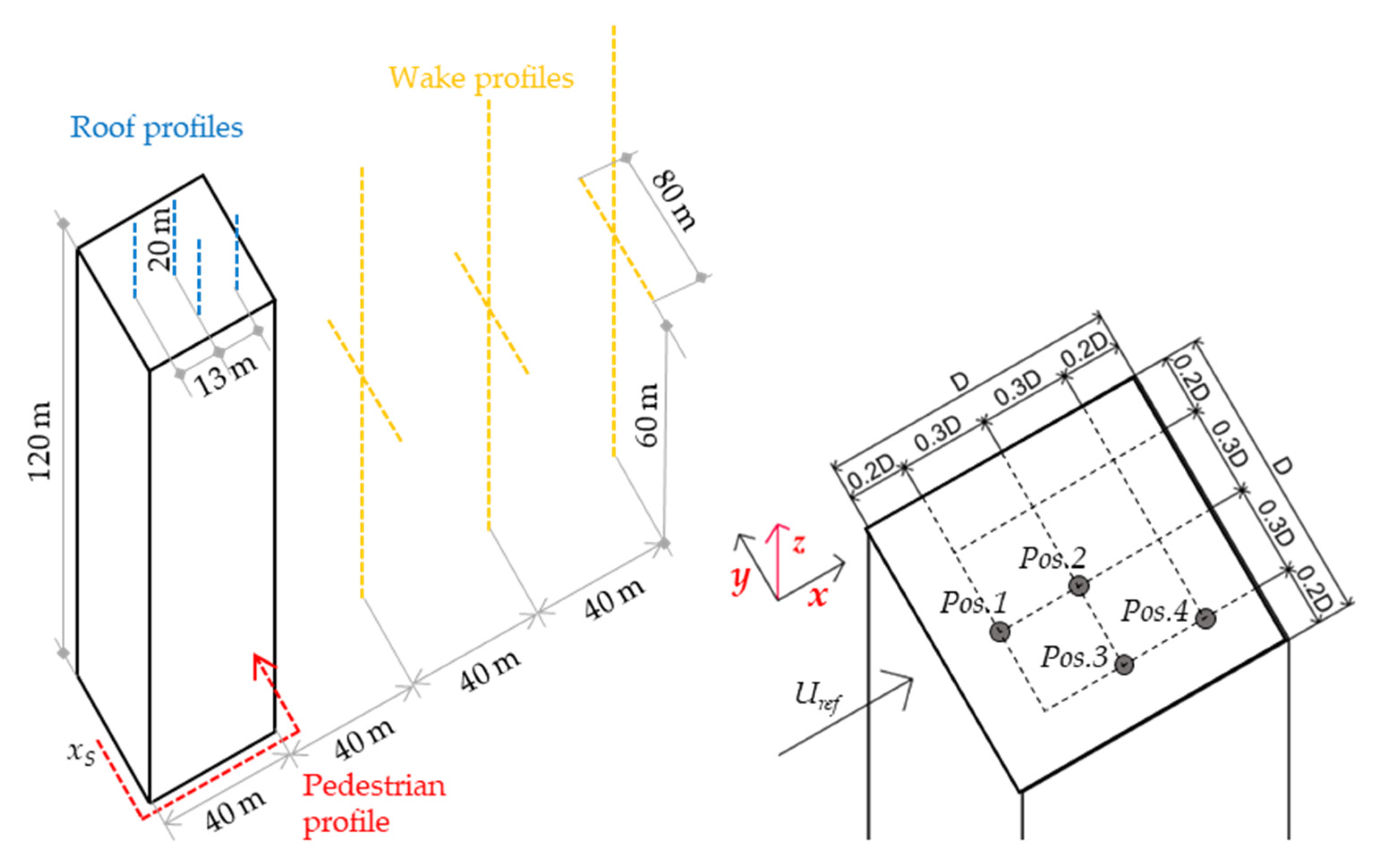
The model is a square prism with a 3:1 aspect ratio, simulating a 1:300 scale high-rise building in atmospheric flow. The height and width of the model are respectively H = 400 mm and D = 133.3 mm. Figure 2 shows the location of measurements above the flat roof of the building. At these locations, profiles of the wind velocity were taken from the numerical simulations. Locations were chosen to highlight the different behavior of the flow around the building, i.e., with profiles placed at the center at the edge or at the corner of the roof, hence in different areas of the separation bubble and cone vortices that form at the roof for this specific wind direction [35].
Figure 3 shows the two different computational domains used in the simulations. The inlet profile from wind tunnel tests was adopted in configuration (a), and the only source of inflow turbulence came from the ground. The steady inlet domain spanned from 2 m = 15D upstream to the model to 4 m = 30D downstream. To avoid blockage issues, the other sizes of the domain were chosen compatibly with the wind tunnel size, i.e., 1.8 m = 13.5D in width and 1.6 m = 12D in height.
The fluctuating configuration (configuration (b)) had the same width and height. However, the turbulent inflow was this time generated by replicating exactly the geometry of the roughness elements present in the wind tunnel. Hence, the domain extended 8.7 m = 65D upstream of the model to 3.8 m = 28.5D downstream. The castellated barrier was placed 1 m from the inlet, and the spires at 2.7 m. The inlet flow was in this case set uniformly at 15 m/s, which allowed for a velocity of Uref~15 m/s at z = H in the model, which was found to be acceptable compared to the experimental case.

2.2. Numerical Setup

This study implemented RANS and LES in combination with the two computational domains to assess the effects of the turbulent inflow on the statistics around the high-rise building model. The turbulent inflow was generated in both LES and RANS using the so-called precursor domain simulation. The upstream part of the wind tunnel, which is responsible for the development of the atmospheric boundary layer (ABL) in an experiment, was modelled in the geometry. This approach counts as a sort of virtual wind tunnel to be modelled [38].
The steady Reynolds-averaged Navier–Stokes (RANS) simulations implemented the k-ω SST turbulence model, which has shown good viability for the estimation of the averaged fields, and it is heavily used in building simulations [11]. It is also known that its performance is hindered by the modelling of fluctuating statistics [5,9,39].
Large eddy simulations (LES) implement the Smagorinsky–Lilly sub-grid scale model that is based on the mixing length concept. A fixed constant is defined to compute sub-grid scale effects, potentially yielding an unphysical behavior. The eddy viscosity reads v s g s = ( C s Δ ) 2 | S ~ | = ( C s Δ ) 2 2 S i j ~ S i j ~ , where S i j is the shear strain rate, and C s   =   0.17 as per indications from literature [40]. The Van Driest function [41] is used in this work to dampen the role of the C s in those regions of the flow where viscosity effects become preponderant. ν s g s is corrected at the wall by substituting the filter size Δ with Δ   =   m i n ( κ y / C s ( 1 e y + / A + ) ; Δ g ) , where A +   =   26 , κ   =   0.41 is the von Kármán constant, and Δ g represents the actual mesh size [40,42,43].
The solver uses the second order central difference scheme for the spatial discretization, the Euler temporal scheme, and high-order discretization for the RANS turbulence model, ensuring a limited numerical dissipation of results [43]. Both RANS and LES were applied to the same block structured hexahedral mesh, which has been constructed so that y+~1, and we chose the blocking strategy in order to limit the along-flow size of the elements to respect the CFL condition which imposes Co < 1. Therefore, the suitable time step for the LES setup was Δ t   =   5 5 .
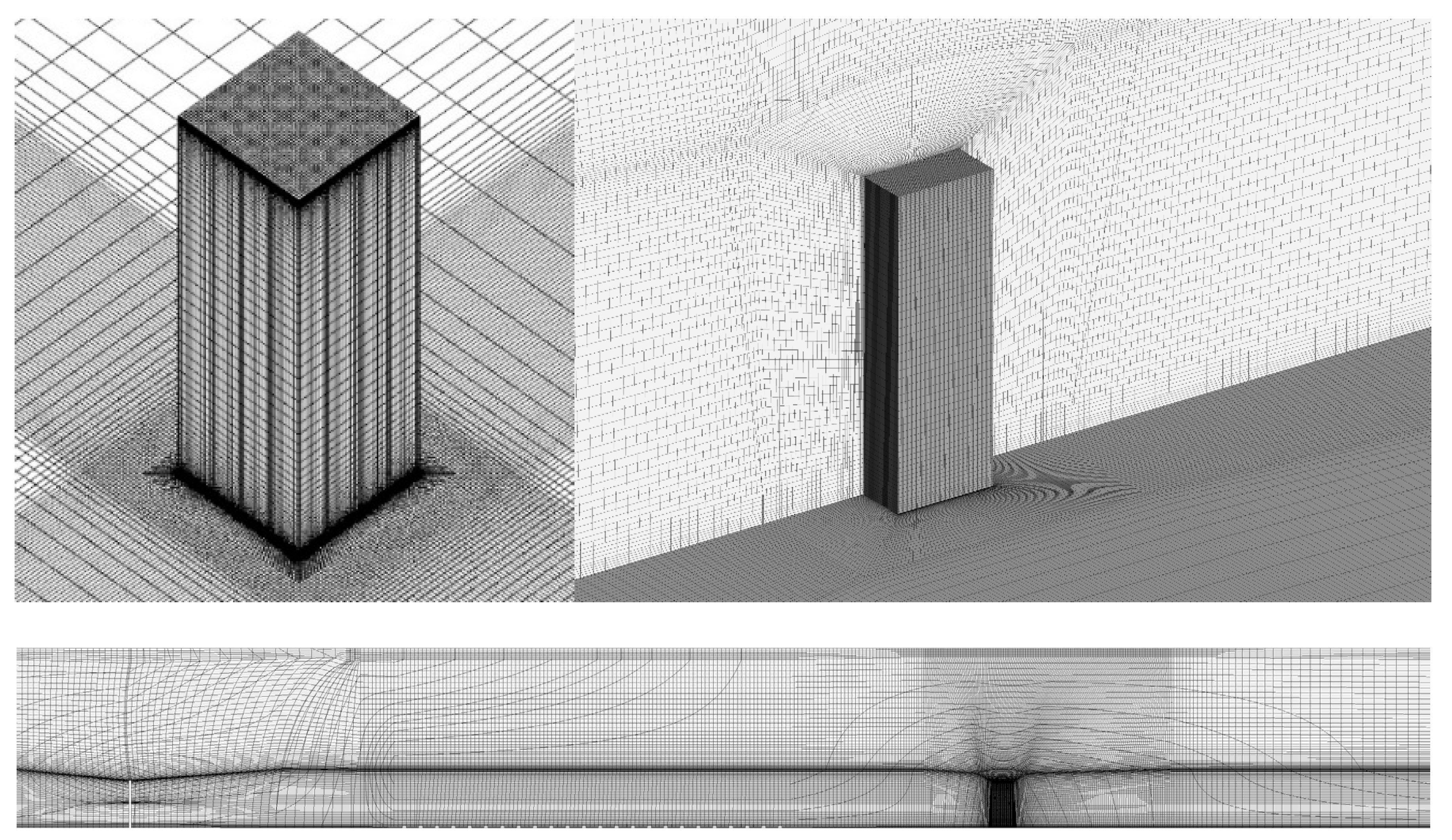
As computational costs need to be contained, a numerical study usually comprises of a thorough mesh sensitivity analysis, which has been here performed and discussed at length in a previous work [44]. Figure 4 shows the computational mesh for the two computational domains with smooth and turbulent inflow conditions. The mesh is created in a similar way, with a highly refined region close to the building and a gradual increase of the cell size to reduce computational costs. The roof region and the pedestrian level are refined further to correctly represent the shear layer features. A detailed account of the mesh resolution and sensitivity analysis is given in [44].
All simulations have been solved suing Ansys CFX v17.2 (ANSYS, Inc. Canonsburg, PA, USA), using 64 processors of the BlueBEAR Windows HPC at the University of Birmingham (discontinued in 2018). RANS steady simulations each took 8 h of computations, while LES required 10 days of computations for ≈6 s of simulation, which corresponds to ≈12 flow-through-times (FTT). The convergence of results within the flow domain was monitored and the chosen FTT was found to be a good compromise between computational costs and accuracy.

3. Results

Results show the flow patterns predicted by RANS and LES, focusing on the different behaviors under smooth and turbulent inflow. The roof region was validated against experimental data and LES results were analyzed in detail to determine the role of the inflow condition. The RANS and LES performances were also compared at other locations, namely, the pedestrian level and wake region, where experimental results are not available.
Previous experimental tests provided the validation test-case for the roof region [35,45], while at other locations the flow was not measured in experiments; however, it is reasonable to consider it to be as accurate as is shown by the roof region due to the similar features (shear and separation) and high quality of the mesh adopted.

3.1. Inflow Profile as Modeled

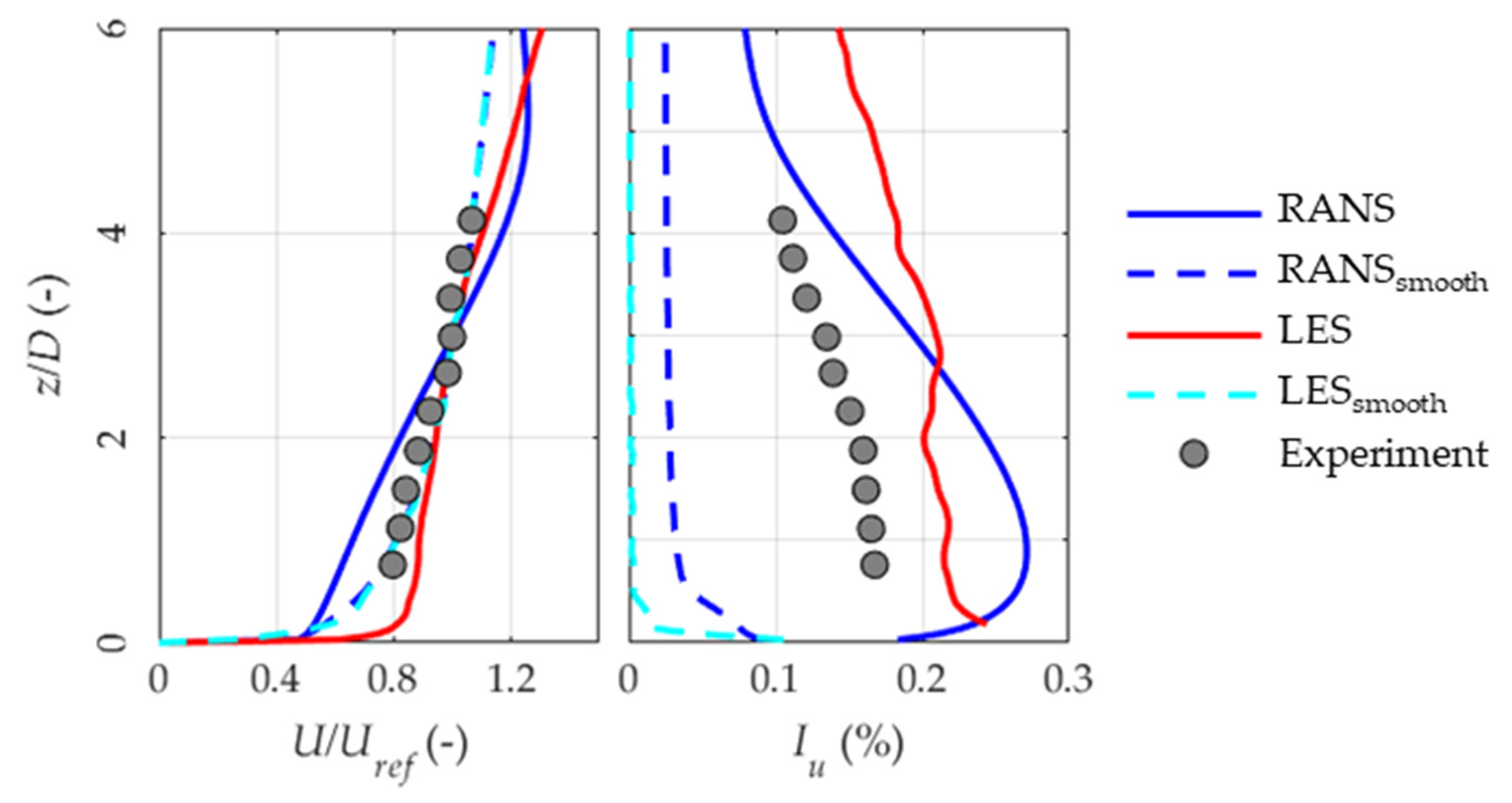
Figure 5 shows the inflow statistics as computed by both smooth and turbulent RANS and LES cases, measured at x = 7D upstream of the model, corresponding to the limits of the turntable of the wind tunnel tests at a distance of x = 0.9 m from the center. The turbulent cases (referred to as RANS and LES) generate the mean wind speed and the turbulence intensity by replicating the wind tunnel geometry, while the smooth cases (RANSsmooth and LESsmooth) have the experimental inflow imposed at the inlet.
Results around the high-rise building model in terms of U/Uref show that RANSsmooth and LESsmooth are able to correctly predict the experimental values. Additionally, LES is also able to predict well the experiments, with a reduced accuracy close to the wall, highlighting the challenging setup, requiring the meshing of the roughness elements in the wind tunnel and the flow upstream of it (normally not available and sometimes not uniform). This might be the reason for RANS missing most of the experimental inlet values. Figure 5 also shows a good match of Iu by RANS and LES, at least in a qualitatively way, with overprediction of about 5%, while RANSsmooth and LESsmooth completely miss the values for U. Therefore, it is evident that inlet turbulence plays a key role in the correct reproduction of turbulence-related values. LES results of Iu are rather optimistic regarding the representations of other high-order features of the inflow; hence, a mismatch of the mean wind speed seems a reasonable compromise. The discussed limitations of each approach, as shown in Figure 5, will be used as references for the interpretation of the upcoming results.

3.2. Numerical Flow Pattern

Surface pressure measurements require a great deal of interpretation of statistics to pair them with a suitable physical explanation based on the flow features. CFD provides the huge advantage of visualizing the flow field, hence immediately explaining the physical behavior and detecting issues in the representation of the flow, especially when using a simplified technique such as RANS.
Figure 6 shows the flow pattern around the high-rise building in the case of a smooth inflow. In this case, the coherent structures of the instantaneous flow are more evident and easily illustrated using the Q-criterion for the detection of vortex cores. Horseshoe vortices are recognizable at the pedestrian level, with two vorticities present upstream of the building. In fact, elongated prisms are known to show upstream multiple vortices near the ground [46,47]. Flow separation is evident from the presence of leading-edge vortices which affect the shear layer between the separation bubble and the free-stream flow. This vorticity is related to the shape of the edge, and the most likely not to be influenced by ambient flow conditions. The leading-edge vorticity evolves into a vortex shedding with periodic behavior, as regions with the same Q-invariant are present at a spacing of roughly 0.025   m or 0.2D, similarly to indications found in literature [48]. In the wake of the building, the vorticity curls up into hairpin vortices that enhance the mixing with the free stream [49]. For this reason, the wake funnels and stretches towards the ground. Some vorticity is dragged downstream of the building with no apparent stretching at roughly 0.5 m or 5D from the building, where the development of the wake is entirely driven by the free stream flow [50]. LES captures this behavior in agreement with the literature, and this can be attributed to the quality of the numerical setup.
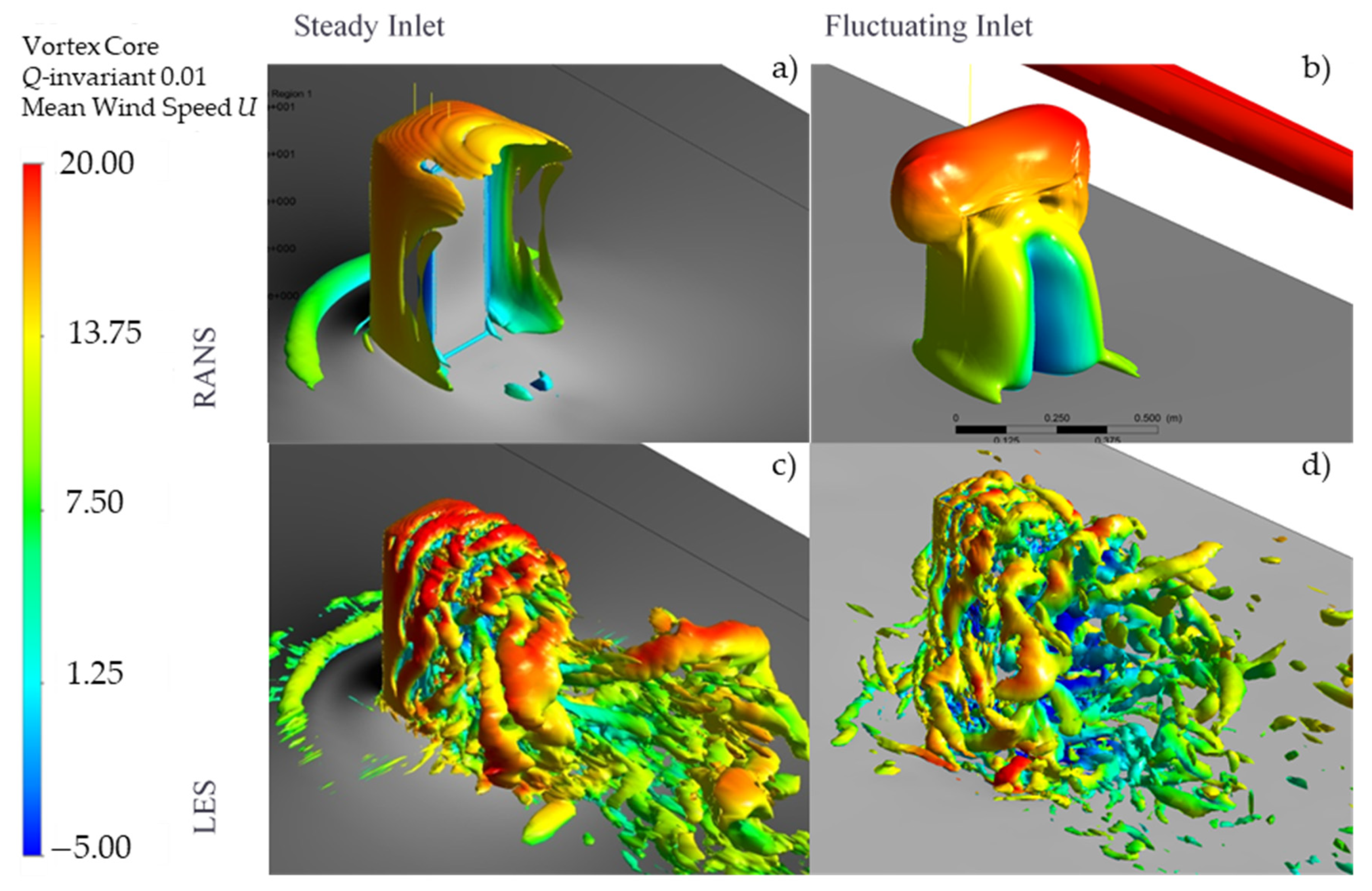
Figure 7 shows the Q-invariant of all considered smooth and turbulent inflow cases for the LES and RANS simulations. As regards the RANS cases, the vortices are rather regular and symmetric, each with a region of vorticity that clearly represents the horseshow vortex around the base of the building (evident for the steady inlet). The RANS case shows instead a large region of vorticity downstream of the building, which indicates an interaction between the separated flow region in the wake with the free-stream flow structures. In fact, a large vortex originating from the inlet spires is noticeable in the top-right corner of the image.
LESsmooth (with steady inlet) visualization is analogous to Figure 6, with horseshoe vortices at the ground upstream the building, and a separated flow above the roof, generating a vortex shedding behind the building, and evolving in large curved vortices in the wake. When the turbulent inflow is introduced, the coherent structures are less evident, as they are disrupted by the smaller coherent structures of the inflow. As the shear layer expands, as per the interaction with the turbulent inlet, turbulence is entrained in the local flow features; hence, the behavior is greatly modified. For example, the wake vortices are much smaller and unorganized, suggesting that the wake dissipates much faster in turbulence [34,51]. However, at the roof the leading-edge vorticity is analogous in both cases. This suggests that when the flow is governed by geometrical features, the presence of the inflow does not affect the behavior. The similar flow patterns of RANSsmooth and LESsmooth simulations confirm that RANS accurately captures the main features of the flow, and this might be sufficient for some engineering applications. Vice versa—with a fluctuating inflow which is likely to affect the flow behavior, especially further from the edges, RANS might not provide sufficient sensitiveness to the interaction, hence potentially affecting the description of local flow phenomena.

3.3. RANS and LES Overprediction of the Roof Region

The roof region of high-rise buildings is critical, as components sensitive to wind, such as solar panels and wind turbines, might be installed there and would need to withstand strong winds. Results are compared in terms of mean wind velocity and turbulence intensity for the positions indicated in Figure 2. Data are normalized using the reference velocity Uref, taken from the inlet wind velocity profile, as computed in the different simulations, at z = H.
Figure 8 shows the mean longitudinal wind velocity U, for which the performances of RANS and LES are comparable. For the fluctuating inflow cases, at lower heights z/D < 0.1, RANS seems to provide a closer match to experimental results compared to LES computations. However, RANS did not detect a separation at position 3. Positions near walls are usually difficult to assess in wind tunnel tests using physical probes (in the present study, hot-wire anemometers). Even if the probe is correctly placed, normally only a limited sensitiveness is available, which might affect the accuracy. Therefore, the lower experimental results are to be taken critical. For instance, a separation seems not to occur at position 2 or position 1, where clearly all numerical techniques indicate there is one. RANS and LES report similar extents of the separation bubble at position 1 and position 2, but cone vortices seem not to be modelled consistently at position 3 and position 4 [35]. As for the smooth inflow, RANSsmooth and LESsmooth provide analogous results throughout the dataset. In general, the extent of the separation bubble seems to be overestimated by both techniques at around 50% larger. This shows how turbulence in the inflow contracts the separation bubble, hence delaying separation and reattachment, which arguably is crucial in the prediction of the flow in the roof region. Figure 8 also shows LES statistics calculated using both the ensemble average (i.e., the average is taken over the entire signal, analogously to RANS theoretical formulation) and the time average (indicated with LESprobes, where the average is done over statistics taken for several signal segments of 1 s duration). Results are consistent, hence reassuring us of the stationarity of the signal, and therefore the comparability of RANS and LES and on the sufficient length of the sample time for LES, in this case T ≈ 6 s for both inflows.
Figure 8 allows one to draw conclusions about the physical behavior of the flow above the roof. The longitudinal velocity U increases by a factor of ≈20% at all positions compared to the reference velocity. Figure 6 seems to indicate that this is position lies above the shear layer between the separated region and the upstream flow, which in previous experiments [44,52] has been consistently known to produce an acceleration of the flow. The above-mentioned increase in the U component of the velocity occurs at z/D~0.15 for position 1 and at z/D~0.2 for position 2, and at z/D~0.3 for other positions. The vertical component W shows a value of ≈50% of the reference velocity at z/D~0.22 in position 1, thereby indicating that at that position any device or component would sustain a highly yawed flow.
Figure 9 shows the longitudinal turbulence intensity. Concerning RANS, Iu was calculated from the turbulent kinetic energy K using the condition of isotropy of the turbulent scales reading I u = 2 / 3 K / U ref . RANSsmooth and LESsmooth (dashed lines) both underestimated turbulence by >60%, and yielded an unphysical position of the Iu peak over the roof, indicating a high position of the shear layer, hence confirming the necessity of introducing turbulence in the inlet to improve accuracy.
On the contrary, LES with inlet turbulence can accurately predict the experimental distribution of Iu for position 1, while overpredicting the peak value at z/D = 0.2 by ≈20% at all other positions. This might be due to the higher turbulence in the inflow. Significantly, the position of the turbulence peak seems to be consistent between LES and the experiment, suggesting that the shear layer extent is governed by geometrical features of the model rather than the turbulence intensity, which, however, seems to govern the intensity of turbulence within the shear layer. On the contrary, RANS with inlet turbulence underestimates both the height and intensity of the turbulence intensity peak at all positions. However, at heights z/D > 0.4, the RANS prediction is consistent with LES and experiments, showing that the inflow turbulence is delivered consistently above the model.

3.4. The Role of Turbulent Inflow in LES Prediction

As LES is most influenced by the correct representation of the turbulent inflow, a detailed analysis of the flow features predicted by LES is proposed in this section, to assess the accuracy of LES in the presence or absence of a turbulent inlet and how it affects the different positions above the roof. Figure 10 shows the vertical turbulence intensity, calculated analogously to the longitudinal one as I w   =   σ w / U ref . Above z/D~0.4, Iw decreased to ≈0.1 in position 1 (matching the one present in the upstream flow), and the same value was reached at z/D~0.5 for position 2. This value is the lowest of the dataset above the rooftop, at a height consistent for the vertical component, and it is quite close to limitations normally posed in the literature of 15% turbulence intensity for the optimal performance of wind turbines. LES overpredicts it consistently with the longitudinal component by about 30% due to the inflow turbulence. At a height of z/D~0.25 (position 1) and ~0.4 (other positions) a turbulence intensity of ≈15% was found in the experimental case, and LES improved the description compared to greater heights. Many engineering applications would see such turbulence as a strong limitation for the serviceability, durability, or feasibility (e.g., wind energy [53]). Figure 10 also suggests that the building affects turbulence intensity up to a height of about ~0.3D, or a third of its width. This is consistent with findings for low-rise buildings in literature [54].
Figure 10 also shows how LES with inlet turbulence is performant in the prediction of three-dimensional flow features. On the contrary, LESsmooth failed in detecting the flow behavior, although at position 4, in the downstream portion of the roof, a higher turbulence intensity was predicted, similarly to experimental data. However, the position of the peak was offset.
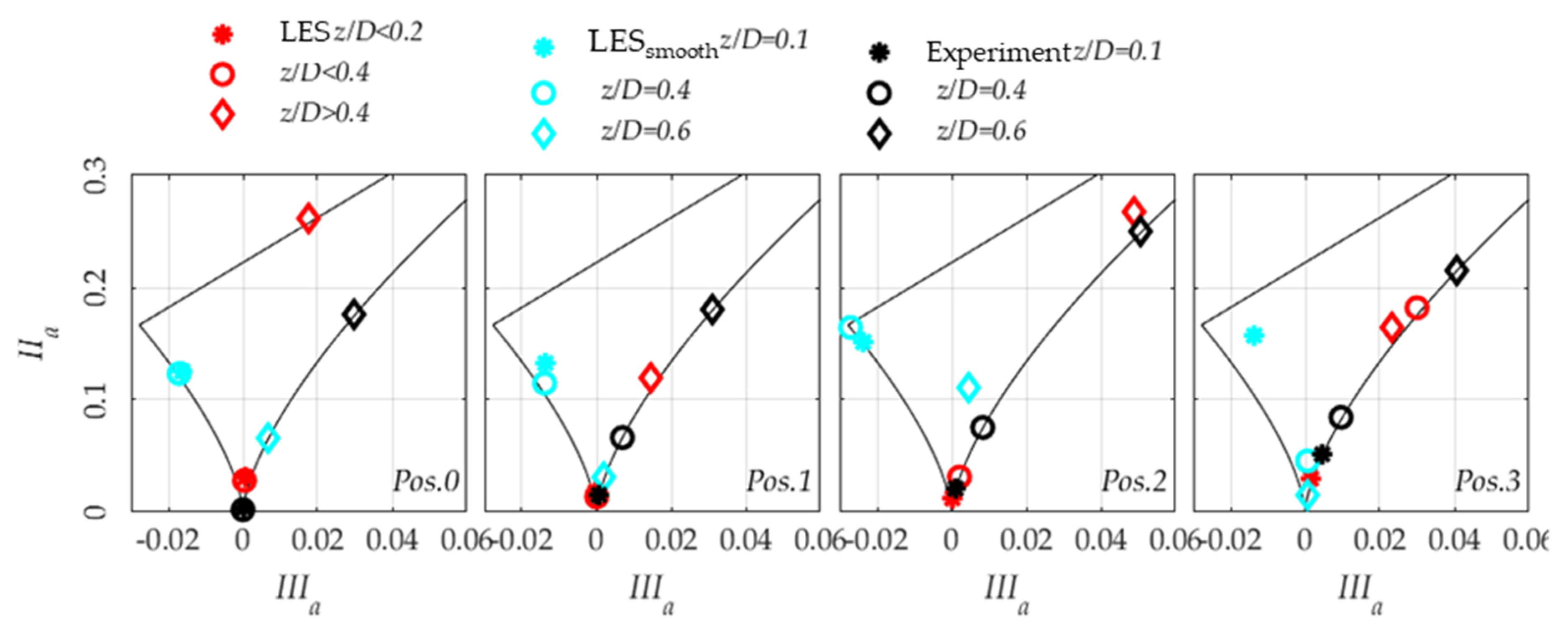
While a discussion on the anisotropy of turbulence might be done using longitudinal and transversal turbulence intensities, there are other methods that use all flow components and yield more accurate interpretations. Figure 11 shows the second and third velocity invariants, I I a   =     u i u j and I I I a   =     u i u j u k , for the measured positions, calculated as explained in [37,55]. Close to the wall, the flow is highly isotropic at all positions, and the anisotropy tends to increase with height for position 1 and position 4, and the flow is rather isotropic also at z/D = 0.1 for position 1. This is consistent with findings in the literature, where it has been found that the anisotropic turbulent inflow stretches around an obstacle, hence increasing its isotropy [51,56]. At position 2, as the separation bubble thickens, the flow is already anisotropic for z/D > 0.2. LES seems to overpredict anisotropy, and this is in line with previous findings on the turbulence intensity [54]. The overprediction is accentuated at position 3 and position 4, which represent the cone vortex behavior [35]. In smooth flow conditions, LESsmooth yields unphysical results, with a high isotropy shown in the freestream and a subsequent anisotropy due to the stretching around the building, with high anisotropy near the wall.
To correctly interpret the unsteady data analyzed in the following figures, a digression on time averaging is considered appropriate. A reliable validation of LES, which is aimed at solving most of the scales in the flow (especially close to walls) requests the comparison between its ~6 s signal with the longer time window that characterizes the experimental data (~120 s), both considering the same scaled geometry and wind tunnel setup. Furthermore, LES time-histories usually need trimming, as the first flow-through times tend to introduce unphysical oscillations in the data [9]. While the stationarity of the signal might result in an accurate evaluation of lower order statistical moments for both long and trimmed signals, for higher-order statistics the accuracy might be limited by the short sample time used. A stationary phenomenon such as the mean wind speed around a bluff body can therefore be predicted accurately with a computationally economic LES, but for other statistics this might not be the case.
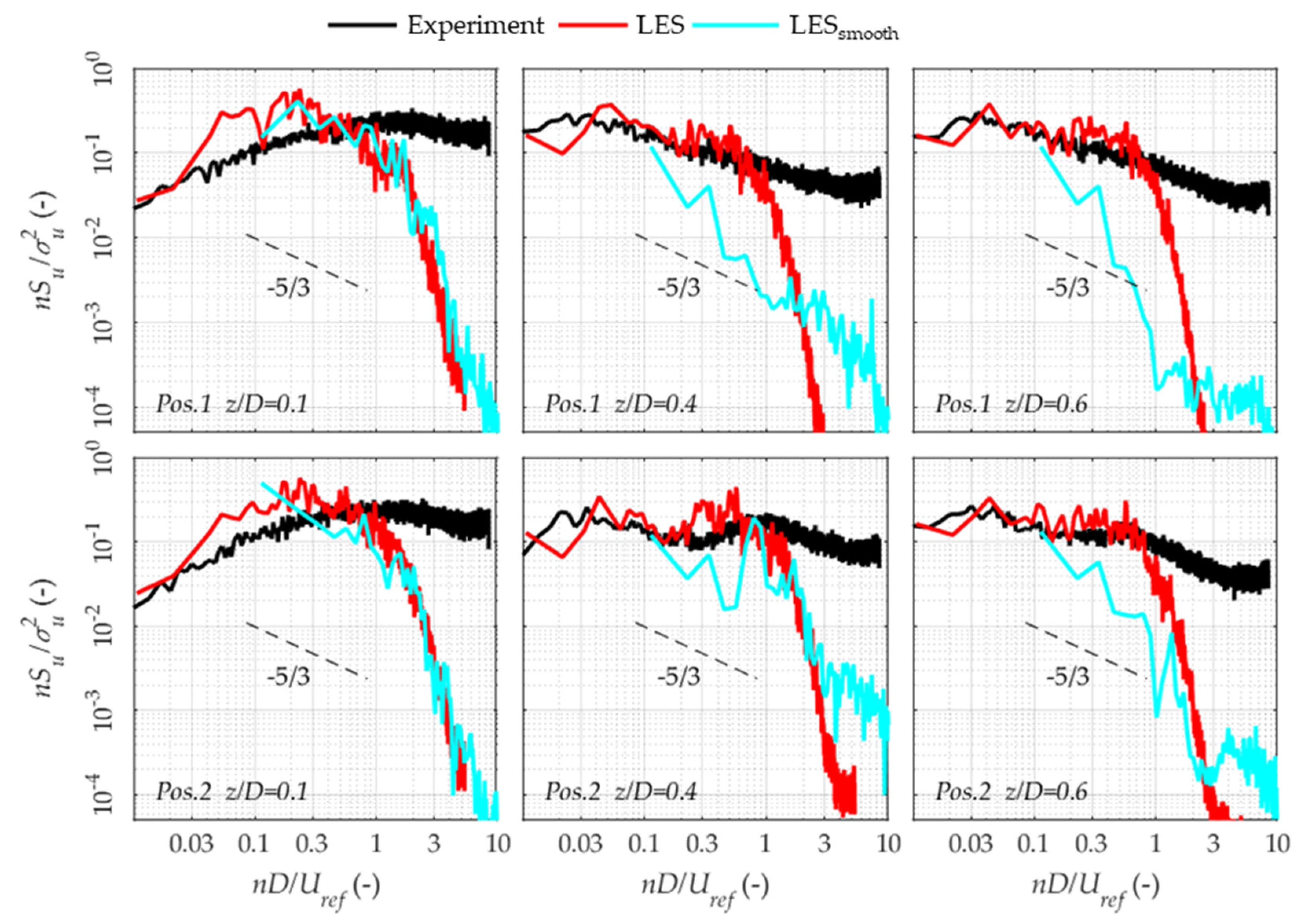
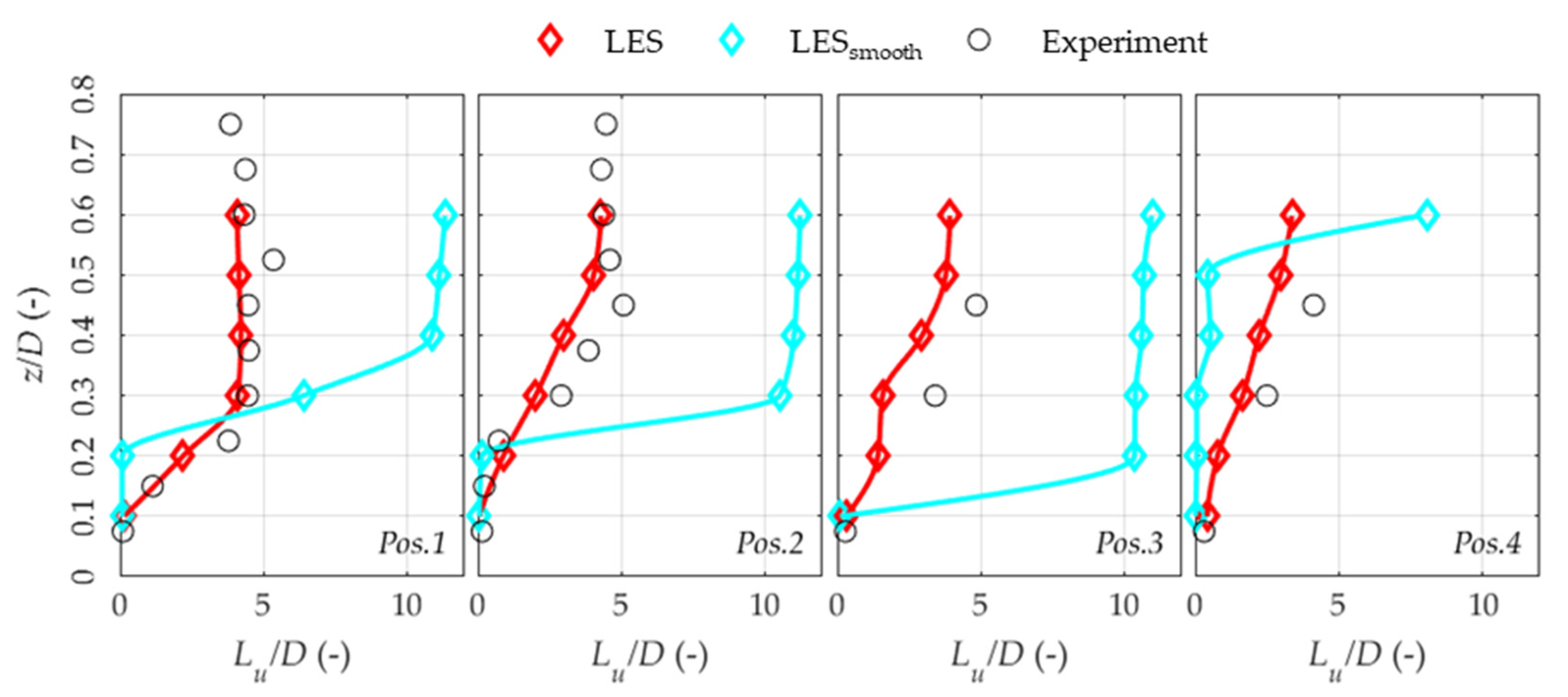
Figure 12 shows the power spectral densities for both positions at experimentally measured heights, close to the roof (z/D = 0.1) and far from it (z/D = 0.4 and z/D = 0.6). Close to the roof, both LES computations in smooth and turbulent inflow gave similar results, thereby indicating that in that that location, turbulence is affected mostly by the leading-edge separation. Up to nD/Uref~0.2, LES presented peaks that could be ascribed to the presence of a vortex shedding, but experiments do not confirm that result. However, the experimental results might be affected by the incapacity of hot-wires in capturing reversed flow. At z/D = 0.6, LES and experimental results are very close for both positions, while LESsmooth fails in capturing any aspect of the behavior. This shows that a longer sample time might be needed in the absence of turbulence, prompting a reflection on the cost-effectiveness of simulations requiring the generation of turbulence at the inlet. It can be also evidenced that LES spectra experienced a sharp fall at nD/Uref > 1, where the filtering of turbulence due to the spatial refinement of the mesh takes place. Nevertheless, the mesh quality was adequate for the present analysis, as a large portion of the sub-inertial range was captured correctly. Those results are confirmed by the calculation of the integral length scale of turbulence using the autocorrelation coefficient, whose values are shown in Figure 13. Close to the ground, LES results do not match experimental ones, while at z/D~0.6 the presence of inlet turbulence is responsible for good matching with experimental data. The effect of the short sample time can be seen, as LES data do not cross the abscissa in a similar way to the experimental data.
Figure 14 shows the longitudinal integral length scale of turbulence Lu/D at roof level positions, which is calculated using the Taylor hypothesis through the integral of the autocorrelation function ρ u up to the first zero-crossing, multiplied by the mean velocity U. The integral length scale shows a steady growth up to a height of z/D~0.22 at position 1 (0.45 at other positions). At greater heights, Lu keeps growing with a different but slower rate up to a maximum point at z/D~0.55, and hints at a slow decrease for even greater heights z/D > 0.7. At z/D~0.55 the probe is in a region of the flow with high shear stresses, which might explain the larger length scale measured in the experimental tests and not captured by the numerical solver. Concerning LESsmooth, results show that the length scale is greatly overestimated for z/D > 0.2. That outcome is coherent with the very low turbulence intensity shown in Figure 9 for the corresponding calculation. On the contrary, LES results with fluctuating inflow match well with experimental data, especially for position 1. At other positions, LES slightly underestimates the length scale by a factor of about 20%: that might be explained considering the overestimation of the turbulence intensity inside of the separation bubble shown in Figure 9, which might be solved either by improving the mesh refinement in the wind tunnel fetch length or increasing the sample time.
Figure 15 shows the probability density functions (PDFs) for position 1 and position 2 at the heights shown in Figure 12. Those PDFs help with understanding the performance of the method with regard to higher-order statistics, especially the behavior of extremes. LES predicts the behavior analogously with wind tunnel experiments at all heights. At position 1 near the wall, the behavior is consistent for LES and the wind tunnel; however, the effect of the short sample time can be noticed with emphasized probability peaks in the PDF, as predicted. A slight mismatch can also be noticed for z / D     0.4 , which is compatible with the higher turbulence intensity generated at the inflow. For smooth inflow, LESsmooth yields an unphysical PDF near the wall, in this case dangerously underestimating the maximum of the distribution. In fact, experimental data suggest fat positive tails, which smooth LESsmooth does not record. At other positions, the behavior is consistent between both LES simulations. At the roof the PDF is generally not normal at all heights, which differs from the atmospheric wind condition normally accepted in the literature [29].
As a general comment, it can be concluded that the LES computation with inlet turbulence demonstrated its reliability to capture most of the turbulent phenomena in the inertial subrange and that it is a reliable and affordable tool for the analysis of the wind resource on roof of a high rise building. The mismatch in the inflow does not impair the accuracy of results, and LES provides a conservative prediction of the turbulent environment. The same conclusion cannot be drawn for LESsmooth.

3.5. RANS over LES Prediction at Pedestrian Level

As simulations are validated at the roof region using experimental measurement, the match between different numerical techniques can be analysed at other locations around the building. The pedestrian level is a particularly challenging area to assess with both experimental and numerical methods. In fact, it is known that it shows variability with the inflow and the building features which is difficult to predict and control [15].
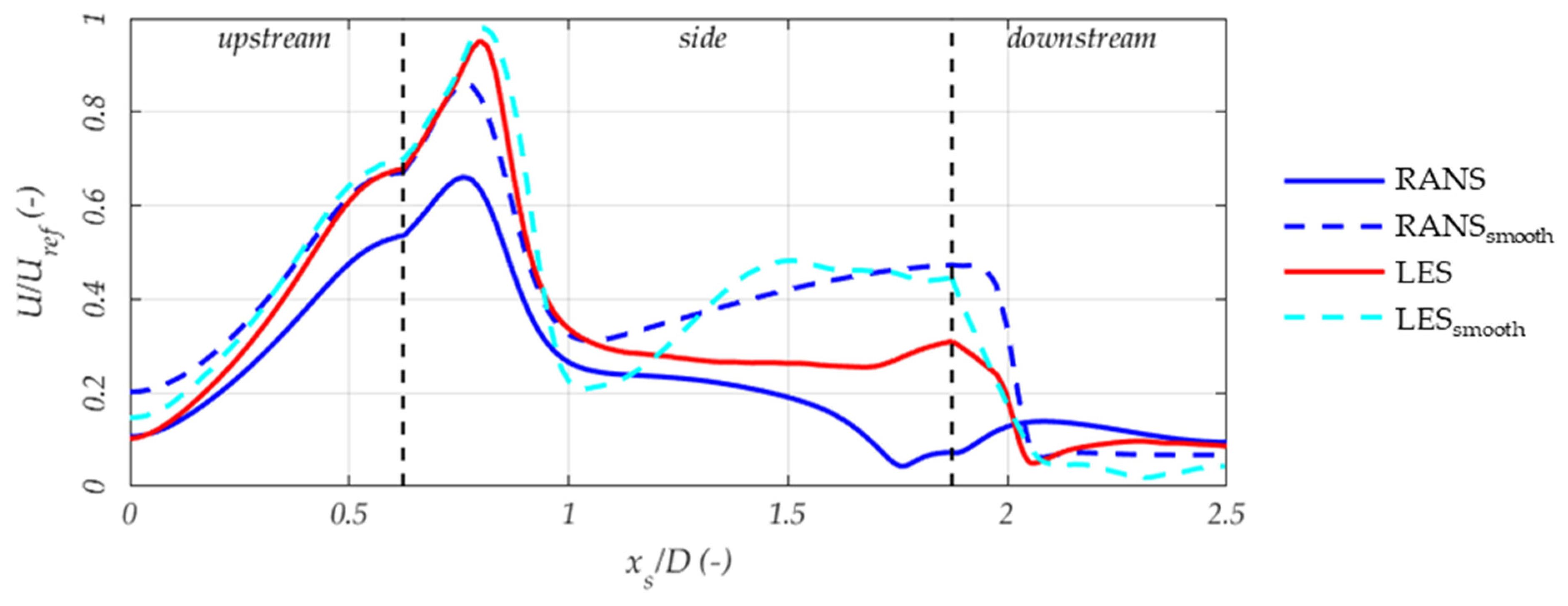
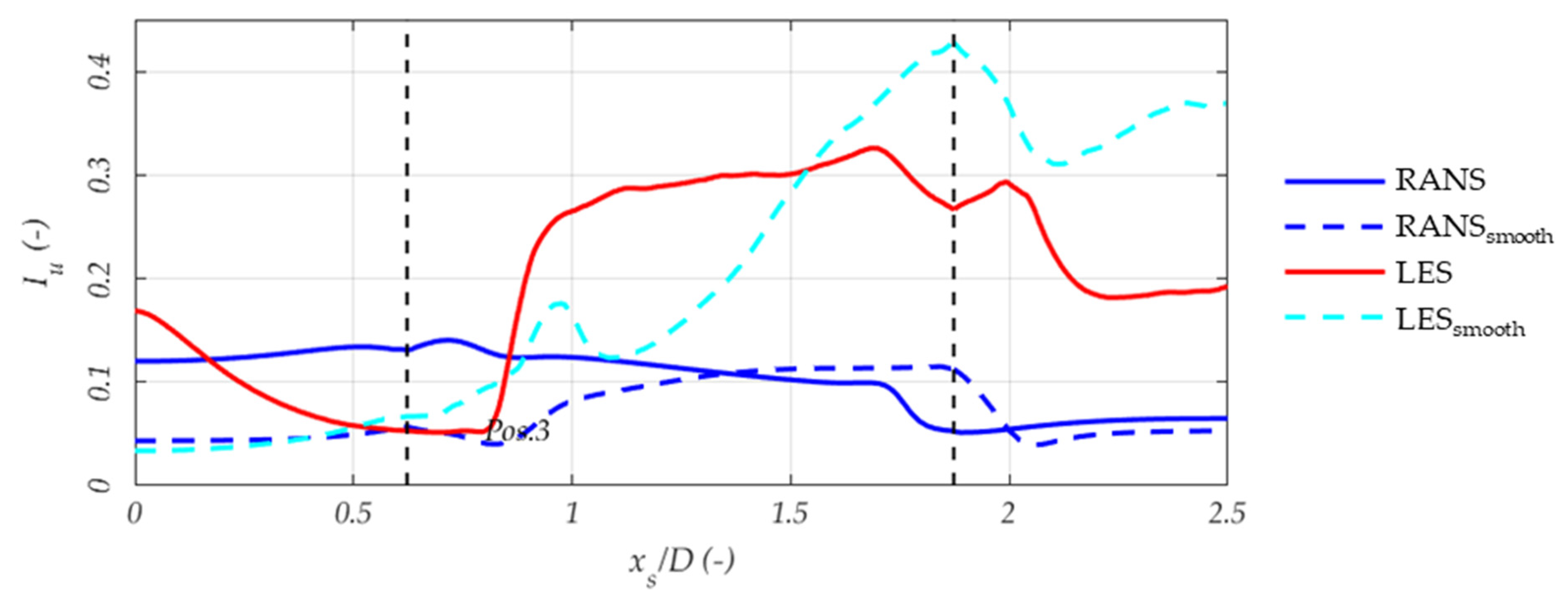
Figure 16 shows the pedestrian environment as predicted by the four cases in this study. The figure shows the pedestrian route as shown in Figure 2, with an upstream streak, a side, and a downstream alignment. For the variability of the flow U refers in this case to the horizontal wind speed, rather than the longitudinal wind velocity as in the rest of the paper. The upstream alignment sees all methods agreeing on the distribution, indicating that the flow features in this area are dominated by the local geometry rather than the ambient turbulence. In the side, a peak is correctly captured by all methods at xS/D~0.8, whose position is again dominated by the leading-edge behavior, as results with smooth and turbulent inflow are consistent. However, RANS and LES predictions differ, with RANS placing the peak at xS/D~0.7. This might depend on the accuracy in the shear layer angle after detachment of the stagnated boundary layer of the downstream façade of the building. The side and downstream alignments show a strong spread. The smooth inflow cases seem to overpredict the pedestrian level wind, and LESsmooth and RANSsmooth are consistent. The turbulent cases show instead a lower wind speed. The RANS case shows the lowest pedestrian wind speed of the dataset. This most probably depends on the higher shear of the inflow wind, which causes a lower wind speed at pedestrian level, when normalising with roof-top wind speed Uref as done for Figure 16.
Figure 17 shows that turbulence intensity proves challenging for the computations, as no agreement at any alignment is present for the studied cases. In the upstream alignment, the turbulence intensity is higher for fluctuating inflow cases and consistently lower for smooth cases. However, RANS and LES do not show the same behavior, with LES reporting a very low turbulence in correspondence to the corner of the building, of which the mean wind speed peak is presented in Figure 16. Experimental results on realistic urban onsets show that this is the case, as areas with strong mean wind speed are normally combined with a lower turbulence intensity [14]. In the separated flow region, on the side and downstream alignments, RANS shows a rather low turbulence intensity of Iu~10%, while smooth and turbulent LES both show intensities >30%. Downstream of the building all techniques agree that a decrease in the turbulence intensity is present, but the LESsmooth shows a very high Iu compared to predictions of other cases.
The pedestrians’ comfort and safety depend on the prediction of the gust wind speed Ug, usually calculated using information from both Figure 16 and Figure 17. Table 1 shows Ug calculated by summating mean wind speed and standard deviation (one of the proposed techniques defined in [57]). RANS seems not to provide conservative results at xS/D = 0.7, where pedestrian safety might be at stake, and in the side alignment it greatly underestimates Ug with respect to RANS. It is interesting to note also that smooth inflow conditions seem to increment significantly pedestrian wind speed in separated flow regions, whereas in regions of coherent gustiness the effect of the inflow is less marked. To give a reference to evaluate results in Table 1, a gust wind speed of 15 m/s is associated with the insurgence of safety issues in pedestrian wind research [57].
Results show that switching to LES is crucial to assess areas of the flow shielded by the building, and the role of the correct inflow is important to ensure the accuracy of the simulations [14,58].

3.6. RANS over LES Prediction in the Wake Region

The wake region is another area of building simulation which has not been fully investigated due to the challenging behavior of the wake, greatly influenced by the shape of buildings and the ambient turbulence, but also due to the difficulty in setting up experimental work to measure wake profiles [9,34,51,56].
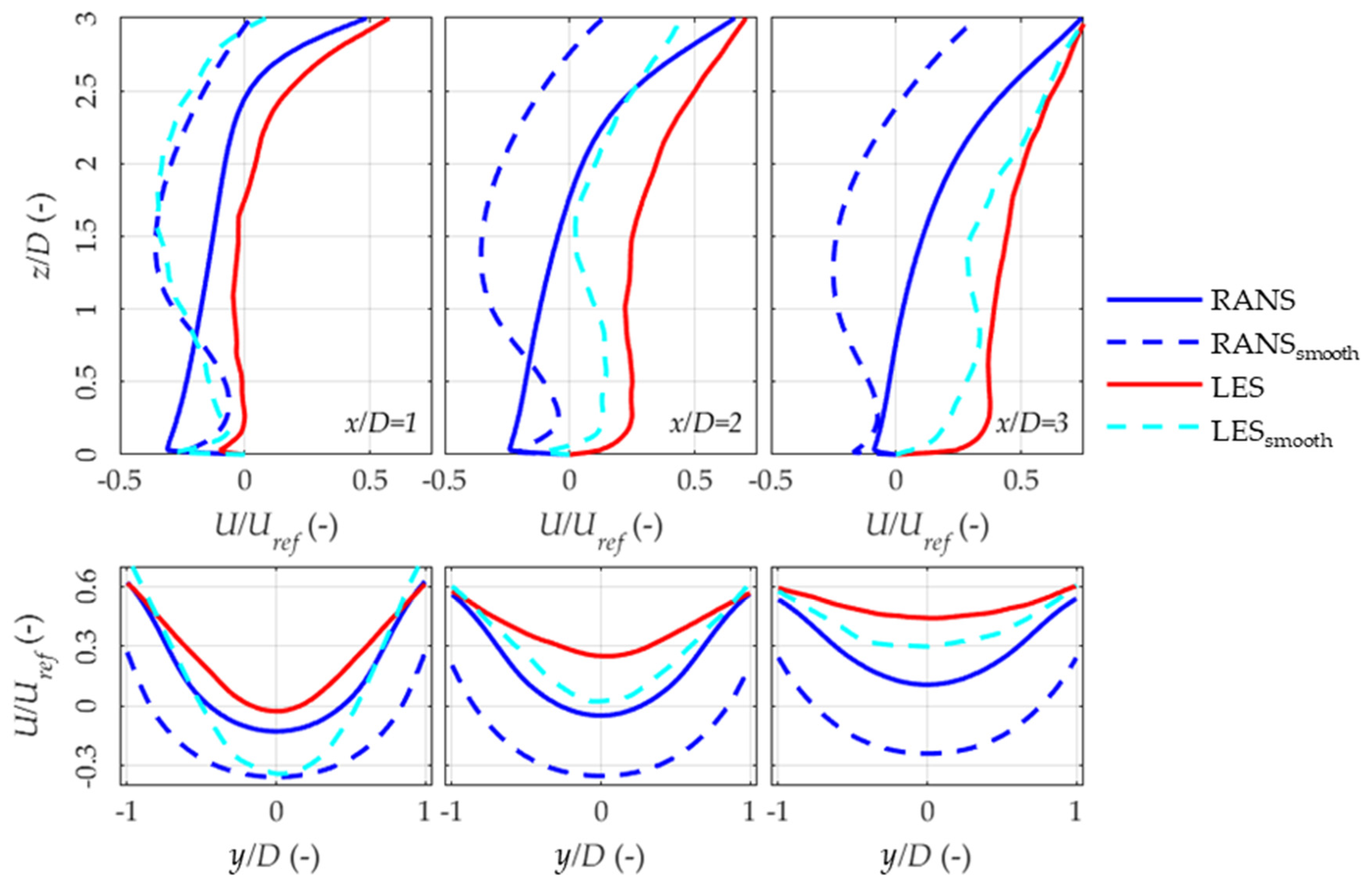
Figure 18 shows the longitudinal wake development at three distances from the building. Both the horizontal and vertical profiles are shown. At x/D = 1 a reversed flow is predicted by all methods. RANSsmooth and LESsmooth show analogous results, with LESsmooth predicting a narrower wake than RANSsmooth. As for the turbulent inflow, RANS shows that the reversed flow region has a height of z/D = 2.5 and a width of y/D~1, whereas LES shows a far less extended separation bubble, z/D~1.7 and y/D~0.3 respectively. At other distances it is evident that LES with turbulent inflow predicts a faster dissipating wake than all other techniques. RANSsmooth shows a very slow wake decay: that is especially evident from the horizontal profiles. Additionally, in the case of fluctuating inflow RANS predicts a slower decay, with the separated flow region still visible at x/D = 3 up to z/D~0.75.
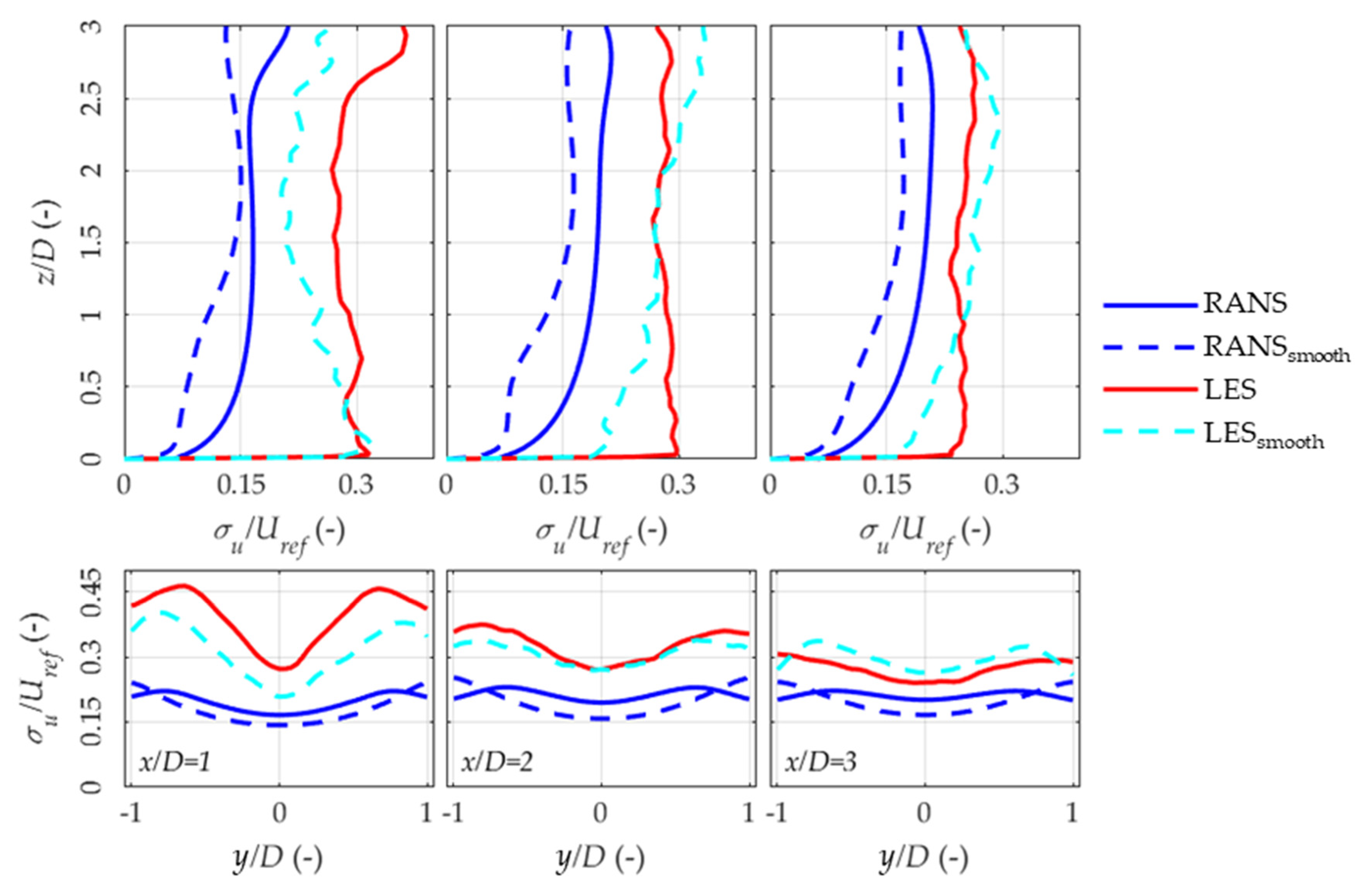
Figure 19 shows the turbulence characteristics measured in the wake region. As the wake decays, turbulence intensity should physically reduce and uniform to the freestream atmospheric flow [9,34]. However, RANS shows an analogous turbulence intensity at the registered distances for both smooth and fluctuating inflow cases, which is an unphysical behavior. Vice versa—LES correctly models the decrease in turbulence intensity for both cases, with the LES in turbulence showing the most rapid decrease. To correctly model the flow behavior, the inclusion of turbulence effects is therefore fundamental, but it does not ensure RANS will improve the behavior significantly in this region.

4. Conclusions

This study provides an assessment of the flow features around a high-rise building, as predicted using RANS and LES with variations of the turbulence characteristics at the inlets of the simulations. The final aim of the research is to understand the possibilities of RANS and the scope of LES in extending wind tunnel results—notoriously limited and expensive, but essential for validation, for several engineering applications.
Results show that there is agreement among the different methodologies in the prediction of the mean velocity, with good matching within those regions of the flow where there is no interaction with the freestream flow, such as close to the leading edge and in the presence of vortex shedding, i.e., in the areas where vorticity is governed directly by the geometric features of the building. However, the matching is problematic in separated or sheared flow regions, where an interaction is present with ambient turbulence.
Although RANS can predict the mean wind velocity, the turbulence intensity is strongly under-predicted, which is problematic considering that many engineering applications specifically require an accurate assessment of the turbulent flow. LES shows instead great flexibility in reproducing a great range of characteristics of the turbulent flow, provided that sufficiently detailed turbulence is provided at the inlet. In general, LES greatly outperforms RANS when a turbulent inlet is provided. However, LES predictions yield unphysical results in the absence of suitable turbulence, strongly underperforming with respect to RANS.
The inclusion of turbulence in the inflow, although usually not considered important in RANS simulations, improves in this case the quality of results throughout the dataset, provided that the mean wind speed at the inflow is accurate. The present study shows that the inclusion of turbulence at the inlet is fundamental also for LES, which in some configurations reports unphysical results, even in those regions of the flow which are governed by the local geometry.
The study also compared the performances of several methods in different flow regions. It is evident that the roof region of high-rise buildings has turbulence characteristics not matching with traditionally accepted values found for the atmospheric boundary layer. In particular, the region spanning ~0.3D from the roof is characterized by reversed, highly turbulent, and low-velocity wind conditions. RANS predicts accurately the flow close to the leading edge when a turbulent inflow is included in the simulation. However, downstream of the roof’s surface, as the separated flow reattaches and a heavy interaction with the turbulent inflow occurs, results do not agree with LES data, which were found to be more sensitive and closely matching with wind tunnel experiments.
At the pedestrian level, all the techniques provide very close matches with each other in the upstream area of the building, where the highest horizontal wind speed occurs. Vice versa—in the side and downstream portion of the pedestrian abscissa investigated in this study, none of the simulations agree on the mean wind speed, and it is sensible that LES provides the closest match to the expected behavior due to its superior performance at the roof region, where a similar flow pattern occurs, with separated and highly turbulent flow.
In the wake region RANS overpredicts the extent of the separated flow at all investigated distances, with LES suggesting a rapid decay of the wake occurs. In this case results do not match at any locations, confirming that RANS only performs accurately in a well-correlated and coherent portion of the flow pattern. Nevertheless, cities are characterized by extensive and multiple interacting wakes from obstacles; hence, it could be interesting to evaluate whether RANS is an option to study urban flow even at those locations close to leading edges in building simulations.

Author Contributions

Conceptualization, G.V. and H.H.; methodology, G.V.; validation, G.V.; formal analysis, G.V.; investigation, G.V. and S.S.; resources, H.H.; data curation, G.V.; writing—original draft preparation, G.V. and S.S.; writing—review and editing, S.S. and D.A.M.; supervision, S.S. and D.A.M.; project administration, S.S. and D.A.M.; funding acquisition, H.H. All authors have read and agreed to the published version of the manuscript.

Funding

The support of the European Commission’s Framework Program Horizon 2020 through the Marie Skłodowska-Curie Innovative Training Networks (ITN) AEOLUS4FUTURE—Efficient harvesting of the wind energy (H2020-MSCA-ITN-2014: grant agreement number 643167) is acknowledged together with the plethora of data and expertise provided by the COST Action TU1804 WINERCOST—Wind Energy to enhance the concept of Smart cities.

Acknowledgments

The authors are grateful to Anina Šarkić-Glumac (University of Luxembourg, LU) and Rüdiger Höffer (Ruhr University of Bochum, DE) for providing the experimental wind tunnel data used to validate the present numerical results.

Conflicts of Interest

The authors declare no conflict of interest. The funders had no role in the design of the study; in the collection, analyses, or interpretation of data; in the writing of the manuscript, or in the decision to publish the results.

References

  1. Haan, F.L.; Kareem, A. Anatomy of Turbulence Effects on the Aerodynamics of an Oscillating Prism. J. Eng. Mech. 2009, 135, 987–999. [Google Scholar] [CrossRef]
  2. Piringer, M.; Joffre, S.; Baklanov, A.; Christen, A.; Deserti, M.; De Ridder, K.; Emeis, S.; Mestayer, P.; Tombrou, M.; Middleton, D.; et al. The surface energy balance and the mixing height in urban areas—Activities and recommendations of COST-Action 715. Bound.-Layer Meteorol. 2007, 124, 3–24. [Google Scholar] [CrossRef]
  3. Franke, J.; Hellsten, A.; Schlunzen, K.H.; Carissimo, B. The COST 732 Best Practice Guideline for CFD simulation of flows in the urban environment: A summary. Int. J. Environ. Pollut. 2011, 44, 419. [Google Scholar] [CrossRef]
  4. Franke, J.; Hirsch, C.; Jensen, A.G.; Krüs, H.W.; Schatzmann, M.; Westbury, P.S.; Miles, S.D.; Wisse, J.A.; Wright, N.G. Recommendations on the use of CFD in wind engineering. In Proceedings of the COST Action C14, Impact of Wind and Storm on City Life Built Environment, Brussels, Belgium, 5–7 May 2004. [Google Scholar]
  5. Blocken, B. Computational Fluid Dynamics for urban physics: Importance, scales, possibilities, limitations and ten tips and tricks towards accurate and reliable simulations. Build. Environ. 2015, 91, 219–245. [Google Scholar] [CrossRef] [Green Version]
  6. Blocken, B. 50 years of Computational Wind Engineering: Past, present and future. J. Wind Eng. Ind. Aerodyn. 2014, 129, 69–102. [Google Scholar] [CrossRef]
  7. Baker, C.J. Wind engineering—Past, present and future. J. Wind Eng. Ind. Aerodyn. 2007, 95, 843–870. [Google Scholar] [CrossRef]
  8. Tamura, T. Towards practical use of LES in wind engineering. J. Wind Eng. Ind. Aerodyn. 2008, 96, 1451–1471. [Google Scholar] [CrossRef]
  9. Blocken, B. LES over RANS in building simulation for outdoor and indoor applications: A foregone conclusion? Build. Simul. 2018, 11, 821–870. [Google Scholar] [CrossRef] [Green Version]
  10. Toja-Silva, F.; Kono, T.; Peralta, C.; Lopez-Garcia, O.; Chen, J. A review of computational fluid dynamics (CFD) simulations of the wind flow around buildings for urban wind energy exploitation. J. Wind Eng. Ind. Aerodyn. 2018, 180, 66–87. [Google Scholar] [CrossRef]
  11. Stathopoulos, T.; Alrawashdeh, H. Urban Wind Energy: A Wind Engineering and Wind Energy Cross-Roads. In Lecture Notes in Civil Engineering; Springer: Cham, Switzerland, 2019; pp. 3–16. [Google Scholar]
  12. Bontempo, R.; Manna, M. The axial momentum theory as applied to wind turbines: Some exact solutions of the flow through a rotor with radially variable load. Energy Convers. Manag. 2017, 143, 33–48. [Google Scholar] [CrossRef]
  13. Moeini, R.; Weston, P.; Tricoli, P.; Dinh, T.Q.; McGordon, A.; Hughes, D. Enhancement of Reliability in Condition Monitoring Techniques in Wind Turbines. In Proceedings of the 2019 23rd International Conference on Mechatronics Technology, ICMT 2019, Fisciano, Italy, 23–26 October 2019; Institute of Electrical and Electronics Engineers Inc.: New York, NY, USA, 2019. [Google Scholar]
  14. Vita, G.; Shu, Z.; Jesson, M.; Quinn, A.; Hemida, H.; Sterling, M.; Baker, C. On the assessment of pedestrian distress in urban winds. J. Wind Eng. Ind. Aerodyn. 2020, 203, 104200. [Google Scholar] [CrossRef]
  15. Blocken, B.; Stathopoulos, T.; van Beeck, J.P.A.J. Pedestrian-level wind conditions around buildings: Review of wind-tunnel and CFD techniques and their accuracy for wind comfort assessment. Build. Environ. 2016, 100, 50–81. [Google Scholar] [CrossRef]
  16. Aly, A.M.; Bitsuamlak, G. Aerodynamics of ground-mounted solar panels: Test model scale effects. J. Wind Eng. Ind. Aerodyn. 2013, 123, 250–260. [Google Scholar] [CrossRef]
  17. Kakimpa, B.; Hargreaves, D.M.; Owen, J.S. An investigation of plate-type windborne debris flight using coupled CFD-RBD models. Part I: Model development and validation. J. Wind Eng. Ind. Aerodyn. 2012. [Google Scholar] [CrossRef] [Green Version]
  18. Kakimpa, B.; Hargreaves, D.M.; Owen, J.S. An investigation of plate-type windborne debris flight using coupled CFD-RBD models. Part II: Free and constrained flight. J. Wind Eng. Ind. Aerodyn. 2012. [Google Scholar] [CrossRef] [Green Version]
  19. Bourriez, F.; Sterling, M.; Baker, C. Windborne debris trajectories in tornado-like flow field initiated from a low-rise building. J. Wind Eng. Ind. Aerodyn. 2020. [Google Scholar] [CrossRef]
  20. Hang, J.; Li, Y.; Sandberg, M.; Buccolieri, R.; Di Sabatino, S. The influence of building height variability on pollutant dispersion and pedestrian ventilation in idealized high-rise urban areas. Build. Environ. 2012, 56, 346–360. [Google Scholar] [CrossRef]
  21. Kim, J.J.; Baik, J.J. Effects of inflow turbulence intensity on flow and pollutant dispersion in an urban street canyon. J. Wind Eng. Ind. Aerodyn. 2003, 91, 309–329. [Google Scholar] [CrossRef]
  22. Fernando, H.J.S.; Zajic, D.; Di Sabatino, S.; Dimitrova, R.; Hedquist, B.; Dallman, A. Flow, turbulence, and pollutant dispersion in urban atmospheres. Phys. Fluids 2010, 22, 1–20. [Google Scholar] [CrossRef]
  23. Sanderse, B.; Pijl, S.P.; Koren, B. Review of computational fluid dynamics for wind turbine wake aerodynamics. Wind Energy 2011, 14, 799–819. [Google Scholar] [CrossRef] [Green Version]
  24. Prospathopoulos, J.M.; Politis, E.S.; Rados, K.G.; Chaviaropoulos, P.K. Evaluation of the effects of turbulence model enhancements on wind turbine wake predictions. Wind Energy 2011, 14, 285–300. [Google Scholar] [CrossRef]
  25. Wu, Y.-T.; Porté-Agel, F. Atmospheric Turbulence Effects on Wind-Turbine Wakes: An LES Study. Energies 2012, 5, 5340–5362. [Google Scholar] [CrossRef]
  26. Moeini, R.; Entezami, M.; Ratkovac, M.; Tricoli, P.; Hemida, H.; Hoeffer, R.; Baniotopoulos, C. Perspectives on condition monitoring techniques of wind turbines. Wind Eng. 2019. [Google Scholar] [CrossRef]
  27. Tanner, K.; Mackenzie, N.; Jones, R.; Lee, Y.K. Aeroacoustic Assessment of Facades. In Proceedings of the ACOUSTICS 2016, Brisbane, Australia, 9–11 November 2016; New Zealand Acoustics: Brisbane, Australia, 2016; p. 11. [Google Scholar]
  28. Zhiyin, Y. Large-eddy simulation: Past, present and the future. Chin. J. Aeronaut. 2015, 28, 11–24. [Google Scholar] [CrossRef] [Green Version]
  29. Ricci, A.; Burlando, M.; Repetto, M.P.; Blocken, B. Simulation of urban boundary and canopy layer flows in port areas induced by different marine boundary layer inflow conditions. Sci. Total Environ. 2019. [Google Scholar] [CrossRef]
  30. Hertwig, D.; Efthimiou, G.C.; Bartzis, J.G.; Leitl, B. CFD-RANS model validation of turbulent flow in a semi-idealized urban canopy. J. Wind Eng. Ind. Aerodyn. 2012, 111, 61–72. [Google Scholar] [CrossRef]
  31. García-Sánchez, C.; Van Tendeloo, G.; Gorlé, C. Quantifying inflow uncertainties in RANS simulations of urban pollutant dispersion. Atmos. Environ. 2017, 161, 263–273. [Google Scholar] [CrossRef]
  32. Baniotopoulos, C.C.; Borri, C.; Stathopoulos, T. Environmental Wind Engineering and Design of Wind Energy Structures; Springer: New York, NY, USA, 2011; Volume 531, p. 352. [Google Scholar]
  33. Flay, R.G.J. Bluff body aerodynamics. In Advanced Structural Wind Engineering; Springer: Tokyo, Japan, 2013; pp. 59–84. ISBN 9784431543374. [Google Scholar]
  34. Irwin, P.A. Bluff body aerodynamics in wind engineering. J. Wind Eng. Ind. Aerodyn. 2008, 96, 701–712. [Google Scholar] [CrossRef]
  35. Hemida, H.; Šarkić Glumac, A.; Vita, G.; Kostadinović Vranešević, K.; Höffer, R. On the Flow over High-rise Building for Wind Energy Harvesting: An Experimental Investigation of Wind Speed and Surface Pressure. Appl. Sci. 2020, 10, 5283. [Google Scholar] [CrossRef]
  36. Šarkić Glumac, A.; Hemida, H.; Höffer, R. Wind energy potential above a high-rise building influenced by neighboring buildings: An experimental investigation. J. Wind Eng. Ind. Aerodyn. 2018, 175, 32–42. [Google Scholar] [CrossRef] [Green Version]
  37. Vita, G. The Effect of Turbulence in the Built Environment on Wind Turbine Aerodynamics. Ph.D. Thesis, University of Birmingham, Birmingham, UK, 2020. [Google Scholar]
  38. Lund, T.S.; Wu, X.; Squires, K.D. Generation of Turbulent Inflow Data for Spatially-Developing Boundary Layer Simulations. J. Comput. Phys. 1998, 140, 233–258. [Google Scholar] [CrossRef] [Green Version]
  39. Ozmen, Y.; Baydar, E.; van Beeck, J.P.A.J. Wind flow over the low-rise building models with gabled roofs having different pitch angles. Build. Environ. 2016, 95, 63–74. [Google Scholar] [CrossRef]
  40. Pope, S.B. Turbulent Flows; Cambridge University Press: Cambridge, UK, 2000; Volume 1, ISBN 0521598869. [Google Scholar]
  41. Van Driest, E.R. On Turbulent Flow near a Wall. J. Aeronaut. Sci. 1956, 23, 1007–1011. [Google Scholar] [CrossRef]
  42. Nicoud, F.; Ducros, F. Subgrid-scale stress modelling based on the square of the velocity gradient tensor. Flow Turbul. Combust. 1999, 62, 183–200. [Google Scholar] [CrossRef]
  43. Ansys Inc. ANSYS CFX-Solver Theory Guide; Ansys Inc.: Canonsburg, PA, USA, 2011. [Google Scholar]
  44. Hemida, H.; Šarkic, A.; Höffer, R. Interference effect of high-rise buildings for wind energy extraction; wind tunnel and numerical investigations. In Proceedings of the 14th International Conference on Wind Engineering, Porto Alegre, Brazil, 21–26 June 2015. [Google Scholar]
  45. Vita, G.; Šarkić-Glumac, A.; Hemida, H.; Salvadori, S.; Baniotopoulos, C. On the Wind Energy Resource above High-Rise Buildings. Energies 2020, 13, 3641. [Google Scholar] [CrossRef]
  46. Baker, C.J. The turbulent horseshoe vortex. J. Wind Eng. Ind. Aerodyn. 1980, 6, 9–23. [Google Scholar] [CrossRef]
  47. Meroney, R.N.; Leitl, B.M.; Rafailidis, S.; Schatzmann, M. Wind-tunnel and numerical modeling of flow and dispersion about several building shapes. J. Wind Eng. Ind. Aerodyn. 1999, 81, 333–345. [Google Scholar] [CrossRef]
  48. Nakamura, Y.; Ohya, Y. Vortex shedding from square prisms in smooth and turbulent flows. J. Fluid Mech. 1986, 164, 77–89. [Google Scholar] [CrossRef]
  49. Buresti, G. Elements of Fluid Dynamics; Imperial College Press: London, UK, 2012; ISBN 1848168896. [Google Scholar]
  50. Zdravkovich, M.M. Flow around Circular Cylinders; Oxford University Press: Oxford, UK, 1997; ISBN 0198563965. [Google Scholar]
  51. Nakamura, Y. Bluff-body aerodynamics and turbulence. J. Wind Eng. Ind. Aerodyn. 1993, 49, 65–78. [Google Scholar] [CrossRef]
  52. Hemida, H. Large-eddy simulation of the above roof flow of a high-rise building for micro-wind turbines. In Proceedings of the 11th UK Conference on Wind Engineering, Nottingham, UK, 11–12 November 2014. [Google Scholar]
  53. IEC 61400-2:2013 Wind Turbines—Part 2: Small Wind Turbines; International Electrotechnical Commission: Geneve, Switzerland, 2013.
  54. Ledo, L.; Kosasih, P.B.; Cooper, P. Roof mounting site analysis for micro-wind turbines. Renew. Energy 2011, 36, 1379–1391. [Google Scholar] [CrossRef]
  55. Jovanović, J. The Statistical Dynamics of Turbulence; Springer: Berlin/Heidelberg, Germany; New York, NY, USA, 2004. [Google Scholar]
  56. Bearman, P.W.; Morel, T. Effect of free stream turbulence on the flow around bluff bodies. Prog. Aerosp. Sci. 1983, 20, 97–123. [Google Scholar] [CrossRef]
  57. Bottema, M. A method for optimisation of wind discomfort criteria. Build. Environ. 2000, 35, 1–18. [Google Scholar] [CrossRef]
  58. Jacob, J.; Sagaut, P. Wind comfort assessment by means of large eddy simulation with lattice Boltzmann method in full scale city area. Build. Environ. 2018, 139, 110–124. [Google Scholar] [CrossRef] [Green Version]
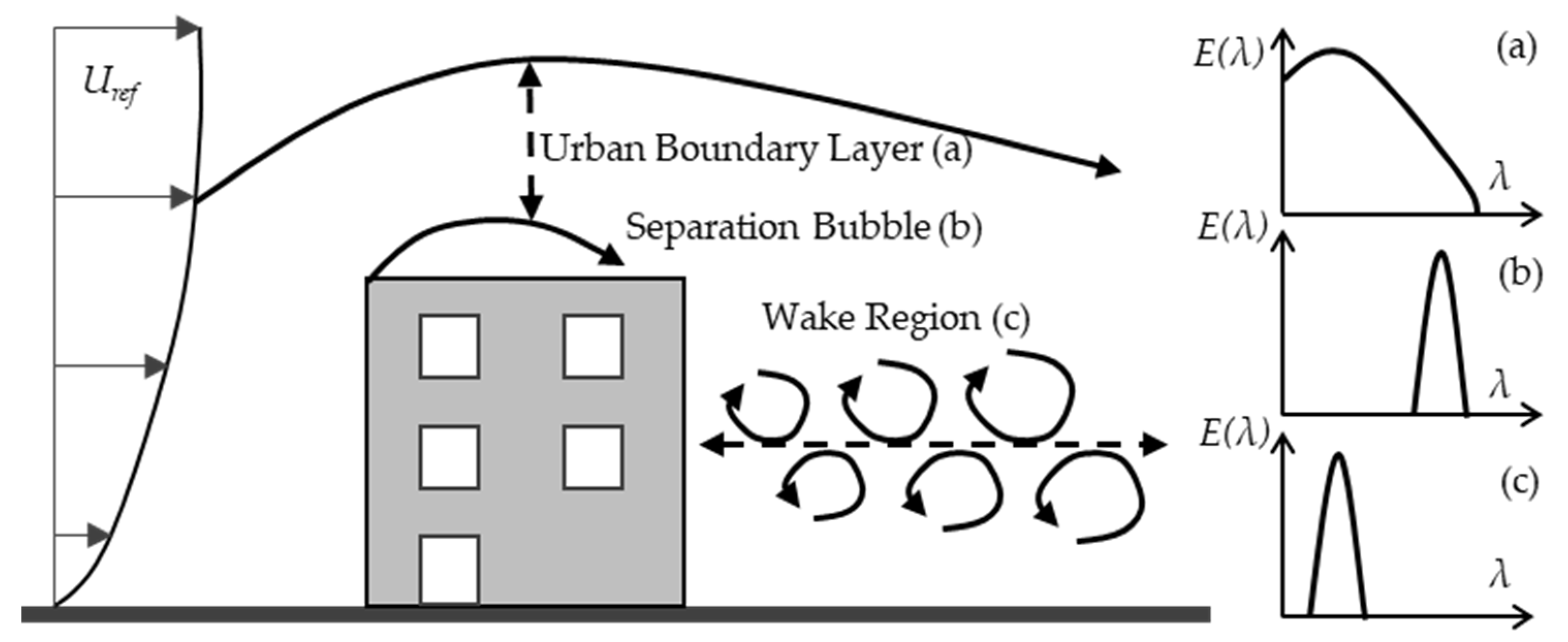
Figure 1. (left) Turbulent structures around a building and (right) associated energy wavelength.
Fluids 05 00233 g001
Figure 2. Numerical model and positions of the measurement profiles. (left) Roof, wake, and pedestrian profiles and their quotes; (right) detail of the roof region positions. xs indicates the abscissa of the pedestrian profile. Quotes are reported in full-scale, where D = 40 m.
Fluids 05 00233 g002
Figure 3. (a) Steady and (b) fluctuating inlet domains for LES.
Fluids 05 00233 g003
Figure 4. Structured block grid of the high-rise building model. On the left, smooth inflow domain.
Fluids 05 00233 g004
Figure 5. Inflow wind speed and its standard deviation, as predicted by the RANS and LES models, compared to the experimental measurements.
Fluids 05 00233 g005
Figure 6. Vortex core visualization (Q invariant 1/s2), with flow pattern identification.
Fluids 05 00233 g006
Figure 7. Flow pattern in terms of velocity-invariant Q = 0.1 around the high-rise buildingin case of (a) RANSsmooth; (b) RANS with fluctuating inlet, (c) LESsmooth, and (d) LES with fluctuating inlet.
Fluids 05 00233 g007
Figure 8. Longitudinal mean velocity values (U) for positions 1, 2, 3, and 4 normalized against Uref. The continuous line refers to the turbulent inlet, and the dashed one to the smooth inlet. LES results were computed using both ensemble averages and time averages from probes for comparison.
Fluids 05 00233 g008
Figure 9. Longitudinal turbulence intensity for positions 1–4. The continuous line refers to the turbulent inlet, and the dashed line to the smooth inlet. LES results were computed using both ensemble averages and time averages from probes for comparison.
Fluids 05 00233 g009
Figure 10. Vertical turbulence intensity for position 1 and position 2.
Fluids 05 00233 g010
Figure 11. Velocity invariants for the assessment of flow anisotropy (LES with smooth and turbulent inlet conditions).
Fluids 05 00233 g011
Figure 12. Power spectral density for position 1 and position 2 at two heights, z/D = 0.1 and 0.6.
Fluids 05 00233 g012
Figure 13. Autocorrelation coefficient for position 1 at two heights, z/D = 0.1 and 0.6.
Fluids 05 00233 g013
Figure 14. Integral length scale of turbulence for position 1 and position 2.
Fluids 05 00233 g014
Figure 15. Probability density function of the longitudinal wind velocity.
Fluids 05 00233 g015
Figure 16. Pedestrian level prediction for the mean horizontal wind speed. xS represents the pedestrian path abscissa shown in Figure 2.
Fluids 05 00233 g016
Figure 17. Pedestrian level prediction of the standard deviation of the horizontal wind speed. xS represents the pedestrian path abscissa shown in Figure 2.
Fluids 05 00233 g017
Figure 18. Prediction of the mean longitudinal wind speed distribution in the wake region. Profiles refer to three distances from the downstream side of the building, namely, x/D = 1, 2, and 3.
Fluids 05 00233 g018
Figure 19. Prediction of the standard deviation of the longitudinal wind speed distribution in the wake region. Profiles refer to three distances from the downstream side of the building, namely, x/D = 1, 2, and 3.
Fluids 05 00233 g019
Table 1. Gust wind speed in m/s, calculated for the different methods at xS/D = 0.7 and xS/D = 1.5.
Gust Wind SpeedxS/DRANSRANSsmoothLESLESsmooth
U g = U + σ u 0.712.0114.5415.9616.93
1.51.748.525.7310.35
Publisher’s Note: MDPI stays neutral with regard to jurisdictional claims in published maps and institutional affiliations.