On a Casson Fluid Motion: Nonuniform Width Symmetric Channel and Peristaltic Flows

Abstract

Widely used for modeling biological fluids flows—in particular, blood vessel flows—a Casson flow is studied in a symmetric channel for which the aspect ratio enables one to use the lubrication approximation. Two flow driving conditions are prescribed: inlet–outlet pressure difference and peristaltic oscillations of the vessel walls. In both cases, starting from mass and momentum balance and using lubrication approximation, we investigate the conditions to be imposed on the driving mechanisms so that the inner plug does not come in touch with the walls. The study of the peristaltic flow is of great importance in view of its applications in physiology (including microcirculation applications).

1. Introduction

During the past several decades, slurries, pastes, rude oil, drilling mud, mineral slurries, suspensions, paint, and materials such as meat extract, frequently encountered in industrial problems, have received increasing attention. The rheological behavior of these materials is usually considered to be viscoplastic, i.e., showing a critical value of stress below which the material does not flow. Such a critical value is usually referred to as yield stress. Viscoplastic materials are also called Bingham plastics, after Bingham [1], who was the first to describe several types of paint in this way in 1919. The models used for these materials included also the Herschel–Bulkley model [2], the Casson model [3] and the Heinz–Casson model [4]. A detailed review of viscoplastic fluids can be found in articles by Bird, Dai and Yarusso [5], Mitsoulis [6], Huilgol [7], and Frigaard and Nouar [8].

All of these models have various practical applications. The Herschel–Bulkley models are used for muds, foams, ceramics, and slurries. The Casson model is widely used to model blood flow [9,10], as it describes blood flow in low shear regions quite well since it captures the nonlinear dependence of viscosity on shear rate. Indeed, the Casson fluid undergoes no deformation until the shear stress is below the critical threshold; above such a threshold, it displays a shear thinning behavior. Merrill et al. [11] found that at shear rates in the range 0.1–1.0 s⁻¹, the Casson constitutive equation fitted the experimental data well. However, we remark that the existence of a yield stress for blood and its use as a material parameter is currently still a controversial issue due to the sensitivity of yield stress measurements in connection to factors that are hardly controllable.

Most of the efforts in the theoretical analyses concern the extent and the shape of yielded/unyielded regions, which are the main feature of viscoplastic materials. A possible approach is the one introduced in [12,13], where the equation of motion of the unyielded part is written in an integral form. According to this method, originally developed by Safronchik [14], the unyielded region is treated as a rigid body of variable mass whose dynamics is governed by the cardinal equations. We remark that the yield surface can be determined using other methods, such as the ones illustrated in [8,15,16,17].

In this paper, we focus on the Casson model and analyze the flow in a symmetric channel with “small” aspect ratio so that the lubrication approximation can be safely used. Lubrication approximation is widely used in a large variety of contexts (see e.g., [18,19,20,21,22]). In particular, the geometrical setting of our study is similar to that studied in [21], where a similar problem is treated for a Newtonian fluid. We analyze the dynamics considering two conditions driving the flow: prescribed inlet–outlet pressure difference and peristalic motion. The case of prescribed inlet discharge has already been analyzed in [23]. We also investigate the conditions ensuring that the inner plug does not come in touch with the walls. Peristaltic flow (for which walls are set in motion by a traveling velocity profile) is studied because of their great importance in understating artery and vein physiology [9,10]. The peristaltic motion of Carreau and Casson nanofluid under the action of a magnetic field and in nonisothermal conditions has been investigated in [24]. The magnetohydrodynamic flow was analyzed in [25], and the dynamics in nanochannels were analyzed in [26,27].

The main aim of this paper is to formulate a sound mathematical model for the motion of a Casson fluid in a vessel with small aspect ratio. As remarked, these flows characterize several applications that span from physiology to geology. Actually, the novelty of this paper is the rigorous application of the momentum equation to the unyielded phase. In the viscoplastic theory, the inner core is in fact a rigid body whose stress cannot be determined. Therefore, in order to get a reliable model, one has to correctly describe its motion equation. This is the key point of our approach. Indeed, the mathematical problem we have obtained is well posed, and this allows us to obtain useful information on the flow. The manuscript is organized as follows. In Section 2, we introduce the mathematical model. The dimensionless form is obtained in Section 3. The asymptotic expansions and the corresponding numerical results are given in Section 5. Finally, the peristaltic flow is investigated in Section 6. Finally, we underline that the study on the peristaltic motion of a Casson fluid can have repercussions in the medical field—in particular, in hemorheology.

2. Mathematical Model

We write the Cauchy stress tensor as $\mathit{T}=-p\mathbf{I}+\mathit{\tau }$, where $\mathit{\tau }$ is its deviatoric traceless part. The constitutive equation for a Casson fluid is given by

$$\left\{\begin{array}{ccc}\mathit{\tau }={\left(\sqrt{\mu }+{\displaystyle \frac{{\sqrt{\tau }}_o}{\sqrt{|\dot{\gamma }|}}}\right)}^2\dot{\gamma },\hfill & & \mathrm{if}\left|\mathit{\tau }\right|⩾{\tau }_o,\\ \dot{\gamma }=0,\hfill & & \mathrm{if}\left|\mathit{\tau }\right|⩽{\tau }_o,\end{array}\right.$$

(1)

where

$$\dot{\gamma }=\nabla \mathbf{v}+\nabla {\mathbf{v}}^T,$$

with $\mathbf{v}$ velocity field and where

$$\left|\dot{\gamma }\right|=\sqrt{{\displaystyle \frac{1}{2}}\dot{\gamma }·\dot{\gamma }},\left|\tau \right|=\sqrt{{\displaystyle \frac{1}{2}}\tau ·\tau }.$$

We investigate the 2D flow in a channel such as the one depicted in Figure 1. The x axis coincides with the channel symmetry line and $y=\pm h\left(x\right)$ are the channel walls.

The velocity field is given by

$$\mathbf{v}(x,y,t)=u(x,y,t){\mathbf{e}}_1+v(x,y,t){\mathbf{e}}_2,$$

and that the fluid is incompressible, i.e., $tr\dot{\gamma }=0$ (isochoric or volume preserving flow). We assume that the yielded part of the flow $\left|\mathit{\tau }\right|⩾{\tau }_o$ and the unyielded part $\left|\mathit{\tau }\right|⩽{\tau }_o$ are separated by the sharp interfaces $y=\pm \sigma (x,t)$, which actually are two free boundaries since their evolution is unknown. Because of symmetry, we may confine our analysis only to the upper part of the channel.

The motion of the unyielded region (schematically depicted in Figure 2)

$${\Omega }_t=\left\{(x,y):0\le x\le L,0\le y\le \sigma (x,t)\right\},$$

obeys to the momentum equation that we write in an integral form (see [28])

$$\underset{{\Omega }_t}{\int }{\displaystyle \frac{\partial }{\partial t}}\left(\rho \mathbf{v}\right)dV+\underset{\partial {\Omega }_t}{\int }\rho \mathbf{v}(\mathbf{v}·\mathbf{n})dS=\underset{\partial {\Omega }_t}{\int }\tau \mathbf{n}dS,$$

(2)

where $\mathbf{n}$ is the normal to ${\Omega }_t$ pointing outward. In the yielded region $\sigma ⩽y⩽h$, the governing equations of the system

$$\left\{\begin{array}{c}{\displaystyle \frac{\partial u}{\partial x}}+{\displaystyle \frac{\partial v}{\partial y}}=0,\hfill \\ \rho \left({\displaystyle \frac{\partial u}{\partial t}}+{\displaystyle \frac{\partial u}{\partial x}}u+{\displaystyle \frac{\partial u}{\partial y}}v\right)=-{\displaystyle \frac{\partial p}{\partial x}}+{\displaystyle \frac{\partial {\tau }_{11}}{\partial x}}+{\displaystyle \frac{\partial {\tau }_{12}}{\partial y}},\hfill \\ \rho \left({\displaystyle \frac{\partial v}{\partial t}}+{\displaystyle \frac{\partial v}{\partial x}}u+{\displaystyle \frac{\partial v}{\partial y}}v\right)=-{\displaystyle \frac{\partial p}{\partial y}}+{\displaystyle \frac{\partial {\tau }_{12}}{\partial x}}+{\displaystyle \frac{\partial {\tau }_{22}}{\partial y}},\hfill \end{array}\right.$$

(3)

where body forces have been neglected.

We remark that Equation (2) is nothing but the first cordinal equation for the rigid core. Because of symmetry, no rotations occur and so (2) is sufficient to determine the translation of the unyielded region.

In the unyielded part, because of symmetry, the motion is a pure translation and the velocity is given by

$$\mathbf{v}=u_c\left(t\right){\mathbf{e}}_1,$$

To write (2) componentwise, we look at Figure 2 where the boundary $\partial {\Omega }_t$ has been divided into four components

$$\partial {\Omega }_t={\mathcal{F}}_1\cup {\mathcal{F}}_2\cup {\mathcal{F}}_3\cup {\mathcal{F}}_4.$$

The first component of Equation (2) is given by

$${\displaystyle \frac{\partial }{\partial t}}\left(\rho u_c\right)\underset{{\Omega }_t}{\int }dV+\rho u_c^2\underset{\partial {\Omega }_t}{\int }({\mathbf{e}}_1·\mathbf{n})dS=\underset{\partial {\Omega }_t}{\int }(\tau \mathbf{n}·{\mathbf{e}}_1)dS,$$

(4)

while the second is given by

$$0=\underset{\partial {\Omega }_t}{\int }(\mathit{\tau }\mathbf{n}·{\mathbf{e}}_2)dS.$$

(5)

The stress tensor is given by

$$\mathit{\tau }=\left(\begin{array}{cc}-p+{\tau }_{11}\hfill & \hfill {\tau }_{12}\\ {\tau }_{12}\hfill & \hfill -p+{\tau }_{22}\end{array}\right),$$

on the surfaces ${\mathcal{F}}_1$ and ${\mathcal{F}}_3$, the only nonzero components of the applied stress are the normal ones, namely

$$\mathit{\tau }{|}_{x=0}=\left(\begin{array}{cc}-p_{in}\hfill & \hfill 0\\ 0\hfill & \hfill -p_{in}\end{array}\right),\tau {|}_{x=L}=\left(\begin{array}{cc}-p_{out}\hfill & \hfill 0\\ 0\hfill & \hfill -p_{out}\end{array}\right),$$

which implies that no torque is applied to the rigid core. Under these hypotheses, setting ${\sigma }_{in}=\sigma (0,t)$, ${\sigma }_{out}=\sigma (L,t)$ and recalling

$$dS=\sqrt{{\sigma }_x^2+1}dx,$$

we find that (5) is automatically fulfilled, while (4) becomes

$$\begin{array}{cc}\hfill 2{\displaystyle \frac{\partial }{\partial t}}\left(\rho u_c\right)\underset{0}{\overset{L}{\int }}\sigma dx =& 2(p_{in}{\sigma }_{in}-p_{out}{\sigma }_{out})+\hfill \\ & +2\underset{0}{\overset{L}{\int }}\left({\sigma }_{x}p-{\sigma }_x{\tau }_{11}+{\tau }_{12}\right){|}_{\sigma }dx.\hfill \end{array}$$

Since $u_c$ depends only on the t variable, integrating by parts, we find

$${\displaystyle \rho \frac{d{u}_c}{dt}\underset{0}{\overset{L}{\int }}\sigma (x,t)dx=\underset{0}{\overset{L}{\int }}{\left.\left[-{\displaystyle \frac{\partial p}{\partial x}}\sigma -{\displaystyle \frac{\partial \sigma }{\partial x}}{\tau }_{11}+{\tau }_{12}\right]\right|}_{\sigma }dx,}$$

(6)

which is the motion equation of the unyielded phase.

To conclude the formulation of the model, we specify the boundary conditions, which are

$$u(x,H,t)=v(x,H,t)=0,(\mathrm{No}-\mathrm{slip}\mathrm{and}\mathrm{impermeability}),$$

(7)

$$u(x,{\sigma }^{+},t)=u_c\left(t\right),v(x,{\sigma }^{+},t)=0,(\mathrm{continuity}\mathrm{of}\mathrm{the}\mathrm{velocity}).$$

(8)

The problem given by (3), (6)–(8) is very complex, even in a simple 2D setting. Analytical solutions can be found when the aspect ratio of the channel is sufficiently small. Indeed, in that case, we can make use of the lubrication approximation to determine a semianalytical solution.

Actually, the main difficulty in solving system (3), (6)–(8) lies in tracking the evolution of $\sigma$, where the constitutive equation exhibits a “singularity”. Indeed, from (1), we extrapolate the following relation between the norms $\left|\mathit{\tau }\right|$ and $|\dot{\gamma }|$, namely

$$\left\{\begin{array}{cc}\left|\mathit{\tau }\right|={\left(\sqrt{\mu |\dot{\gamma }|}+\sqrt{{\tau }_o}\right)}^2\hfill & \hfill |\dot{\gamma }|>0,\\ \left|\mathit{\tau }\right|\in [0,{\tau }_o]\hfill & \hfill |\dot{\gamma }|=0,\end{array}\right.$$

(9)

which is a graph exhibiting a singularity in $|\dot{\gamma }|=0$. A typical way to bypass this difficulty is generally to smooth the constitutive relationship (see [6,29,30] for more details). The positive point of the smoothing methods is their simple implementation in numerical solvers. For example, many commercially CFD codes include inner regularization routines, which smooth the viscosity. However, the issue of the convergence of the yield surface determined using a smoothed constitutive model toward the one of the exact model is far to be settled down. Indeed, to prove that the regularized yield surface converges to the one obtained, solving the exact model requires a uniform convergence results which, at least in the authors’ knowledge, has not yet been obtained.

3. Nondimensional Formulation

We rescale the system as

$$x=L\tilde{x},y=ϵL\tilde{y},t=\left({\displaystyle \frac{L}{U}}\right)\tilde{t},u=U\tilde{u},v=ϵU\tilde{v},u_c=U{\tilde{u}}_c,$$

$$h=H\tilde{h},\sigma =H\tilde{\sigma },\tau =\left({\displaystyle \frac{\mu U}{H}}\right)\tilde{\tau },\dot{\gamma }=\left({\displaystyle \frac{U}{H}}\right)\dot{\tilde{\gamma }},p=\left({\displaystyle \frac{\mu UL}{H^2}}\right)\tilde{p},$$

where L is the length of the channel, $H={max}_{[0,L]}h\left(x\right)$, and

$$ϵ={\displaystyle \frac{H}{L}}\ll 1,$$

(10)

is the aspect ratio. We also introduce the dimensionless half-discharge as

$${\displaystyle Q={\displaystyle \frac{1}{UH}}\underset{0}{\overset{H}{\int }}udy=\underset{0}{\overset{1}{\int }}\tilde{u}d\tilde{y}.}$$

(11)

With this scaling, we get

$$\dot{\tilde{\gamma }}=\left[\begin{array}{cc}2ϵ{\displaystyle \frac{\partial \tilde{u}}{\partial \tilde{x}}}\hfill & \hfill \left({\displaystyle \frac{\partial \tilde{u}}{\partial \tilde{y}}}+{ϵ}^2{\displaystyle \frac{\partial \tilde{v}}{\partial \tilde{x}}}\right)\\ \left({\displaystyle \frac{\partial \tilde{u}}{\partial \tilde{y}}}+{ϵ}^2{\displaystyle \frac{\partial \tilde{v}}{\partial \tilde{x}}}\right)\hfill & \hfill 2ϵ{\displaystyle \frac{\partial \tilde{v}}{\partial \tilde{y}}}\end{array}\right],$$

$$\tilde{\tau }={\left[1+{\displaystyle \frac{\sqrt{B}}{\sqrt{|\dot{\tilde{\gamma }}|}}}\right]}^2\left[\begin{array}{cc}2ϵ{\displaystyle \frac{\partial \tilde{u}}{\partial \tilde{x}}}\hfill & \hfill \left({\displaystyle \frac{\partial \tilde{u}}{\partial \tilde{y}}}+{ϵ}^2{\displaystyle \frac{\partial \tilde{v}}{\partial \tilde{x}}}\right)\\ \left({\displaystyle \frac{\partial \tilde{u}}{\partial \tilde{y}}}+{ϵ}^2{\displaystyle \frac{\partial \tilde{v}}{\partial \tilde{x}}}\right)\hfill & \hfill 2ϵ{\displaystyle \frac{\partial \tilde{v}}{\partial \tilde{y}}}\end{array}\right],$$

where

$$B=\left({\displaystyle \frac{{\tau }_{o}H}{\mu U}}\right),$$

is the Bingham number and where

$$\left|\dot{\tilde{\gamma }}\right|=\sqrt{2{ϵ}^2\left[{\left({\displaystyle \frac{\partial \tilde{u}}{\partial \tilde{x}}}\right)}^2+{\left({\displaystyle \frac{\partial \tilde{v}}{\partial \tilde{y}}}\right)}^2\right]+{\left({\displaystyle \frac{\partial \tilde{u}}{\partial \tilde{y}}}+{ϵ}^2{\displaystyle \frac{\partial \tilde{v}}{\partial \tilde{x}}}\right)}^2}.$$

(12)

Equation (3)₁ becomes

$${\displaystyle \frac{\partial \tilde{u}}{\partial \tilde{x}}}+{\displaystyle \frac{\partial \tilde{v}}{\partial \tilde{y}}}=0,$$

while Equations (3)_2,3 become

$$\left\{\begin{array}{c}ϵ\mathsf{Re}\left({\displaystyle \frac{\partial \tilde{u}}{\partial \tilde{t}}}+{\displaystyle \frac{\partial \tilde{u}}{\partial \tilde{x}}}\tilde{u}+{\displaystyle \frac{\partial \tilde{u}}{\partial \tilde{y}}}\tilde{v}\right)=-{\displaystyle \frac{\partial \tilde{p}}{\partial \tilde{x}}}+ϵ{\displaystyle \frac{\partial {\tilde{\tau }}_{11}}{\partial \tilde{x}}}+{\displaystyle \frac{\partial {\tilde{\tau }}_{12}}{\partial \tilde{y}}},\hfill \\ {ϵ}^3\mathsf{Re}\left({\displaystyle \frac{\partial \tilde{v}}{\partial \tilde{t}}}+{\displaystyle \frac{\partial \tilde{v}}{\partial \tilde{x}}}\tilde{u}+{\displaystyle \frac{\partial \tilde{v}}{\partial \tilde{y}}}\tilde{v}\right)=-{\displaystyle \frac{\partial \tilde{p}}{\partial \tilde{y}}}+{ϵ}^2{\displaystyle \frac{\partial {\tilde{\tau }}_{12}}{\partial \tilde{x}}}+ϵ{\displaystyle \frac{\partial {\tilde{\tau }}_{22}}{\partial \tilde{y}}},\hfill \end{array}\right.$$

(13)

where

$$\mathsf{Re}={\displaystyle \frac{\rho UH}{\mu }},$$

is the Reynolds number. Finally, Equation (6) becomes

$${\displaystyle ϵ\mathsf{Re}\left[{\displaystyle {\dot{\tilde{v}}}_c\underset{0}{\overset{1}{\int }}\tilde{\sigma }(\tilde{x},\tilde{t})d\tilde{x}}\right]=\underset{0}{\overset{1}{\int }}{\left.\left[-{\displaystyle \frac{\partial \tilde{p}}{\partial \tilde{x}}}\tilde{\sigma }-ϵ{\displaystyle \frac{\partial \tilde{\sigma }}{\partial \tilde{x}}}{\tilde{\tau }}_{11}+{\tilde{\tau }}_{12}\right]\right|}_{\tilde{\sigma }}d\tilde{x}.}$$

4. Leading Order Approximation

Let us now focus on the leading order approximation. In practice, we simplify the model retaining only those terms that do not contain $ϵ$. This is the so-called lubrication approximation. Dropping the tildes to keep the notation as light as possible, we have

$$\left\{\begin{array}{cc}{\displaystyle \frac{\partial u}{\partial x}}+{\displaystyle \frac{\partial v}{\partial y}}=0,\hfill & \\ {\displaystyle \frac{\partial {\tau }_{12}}{\partial y}}={\displaystyle \frac{\partial p}{\partial x}},\hfill & (\mathrm{Yielded}\mathrm{phase})y\in [\sigma ,h],\\ {\displaystyle \frac{\partial p}{\partial y}}=0,\hfill \end{array}\right.$$

(14)

$$\left\{\begin{array}{cc}{\displaystyle \underset{0}{\overset{1}{\int }}{\left.\left[-{\displaystyle \frac{\partial p}{\partial x}}\sigma +{\tau }_{12}\right]\right|}_{\sigma }dx=0,}\hfill & \\ & \hfill (\mathrm{Unyielded}\mathrm{phase})y\in [0,\sigma ],\\ u=u_{c}v=0,\hfill & \end{array}\right.$$

(15)

where

$${\tau }_{12}={\displaystyle \frac{\partial u}{\partial y}}{\left[1+{\displaystyle \frac{\sqrt{B}}{\sqrt{\left|{\displaystyle \frac{\partial u}{\partial y}}\right|}}}\right]}^2.$$

(16)

The yield condition is given by

$$|\dot{\gamma }{|}_{\sigma }={\left|{\displaystyle \frac{\partial u}{\partial y}}\right|}_{\sigma }=0.$$

(17)

Recalling that in the upper yielded part $\partial u/\partial y<0$, we find

$${\displaystyle \frac{\partial u}{\partial y}}=-\left|{\displaystyle \frac{\partial u}{\partial y}}\right|,$$

so that (16) rewrites as

$${\tau }_{12}=-{\left[\sqrt{\left|{\displaystyle \frac{\partial u}{\partial y}}\right|}+\sqrt{B}\right]}^2,$$

(18)

which, by virtue of (17), gives

$${\tau }_{12}{|}_{\sigma }=-B.$$

From (14)₃, we see that $p=p(x,t)$ so that, integrating (14)₂ between $\sigma$ and y, we find

$${\tau }_{12}=-B+{\displaystyle \frac{\partial p}{\partial x}}(y-\sigma ).$$

(19)

Inserting (18) into (19), we get

$${\left[\sqrt{\left|{\displaystyle \frac{\partial u}{\partial y}}\right|}+\sqrt{B}\right]}^2=B+{\displaystyle \frac{\partial p}{\partial x}}(\sigma -y),$$

and hence

$${\displaystyle \frac{\partial u}{\partial y}}=-{\left(\sqrt{B+{\displaystyle \frac{\partial p}{\partial x}}(\sigma -y)}-\sqrt{B}\right)}^2.$$

(20)

Assuming that the pressure drop $\Delta p>0$, we expect $p_x<0$ so that $p_x(\sigma -y)>0$ in the yielded phase. Integrating (20) between y and h and exploiting (7), we find

$${\displaystyle u=\underset{y}{\overset{h}{\int }}{\left(\sqrt{B+{\displaystyle \frac{\partial p}{\partial x}}(\sigma -\xi )}-\sqrt{B}\right)}^{2}d\xi .}$$

Setting

$$\mathcal{P}={\displaystyle \frac{p}{B}},$$

(21)

we may rewrite u as

$${\displaystyle {\displaystyle \frac{u}{B}}=\underset{y}{\overset{h}{\int }}{\left(\sqrt{1+{\mathcal{P}}_x(\sigma -\xi )}-1\right)}^{2}d\xi ,}$$

which, after some algebra, gives

$$\begin{array}{cc}\hfill {\displaystyle \frac{u}{B}}=& {\displaystyle \frac{{\mathcal{P}}_x}{2}}\left[{(\sigma -y)}^2-{(\sigma -h)}^2\right]+2(h-y)+\hfill \\ & +{\displaystyle \frac{4}{3{\mathcal{P}}_x}}\left[{({\mathcal{P}}_x(\sigma -h)+1)}^{3/2}-{({\mathcal{P}}_x(\sigma -y)+1)}^{3/2}\right].\hfill \end{array}$$

(22)

Evaluating (22) on $y=\sigma$, we find

$$-{\displaystyle \frac{u_c}{B}}={\displaystyle \frac{{\mathcal{P}}_x}{2}}{(\sigma -h)}^2+2(\sigma -h)-{\displaystyle \frac{4}{3{\mathcal{P}}_x}}\left[{({\mathcal{P}}_x(\sigma -h)+1)}^{3/2}-1\right],$$

(23)

where we recall that $u_c$ does not depend on x. Rearranging (22) and (23), we find

$${\displaystyle \frac{u}{u_c}}=\left[1-{\displaystyle \frac{\frac{{\mathcal{P}}_x}{2}{(\sigma -y)}^2+2(\sigma -y)-\frac{4}{3{\mathcal{P}}_x}\left[{({\mathcal{P}}_x(\sigma -y)+1)}^{3/2}-1\right]}{\frac{{\mathcal{P}}_x}{2}{(\sigma -h)}^2+2(\sigma -h)-\frac{4}{3{\mathcal{P}}_x}\left[{({\mathcal{P}}_x(\sigma -h)+1)}^{3/2}-1\right]}}\right],$$

(24)

so that we can easily check that ${u|}_h=0$ and ${u|}_{\sigma }=u_c$, i.e., (7) and (8) are fulfilled.

We now exploit the constraint of incompressibility $u_x+v_y=0$. Recalling the conditions ${v|}_h{=v|}_{\sigma }=0$, we find

$${\displaystyle 0=\underset{\sigma }{\overset{h}{\int }}{\displaystyle \frac{\partial v}{\partial y}}dy=-\underset{\sigma }{\overset{h}{\int }}{\displaystyle \frac{\partial u}{\partial x}}dy.}$$

As a consequence,

$${\displaystyle \frac{\partial }{\partial x}}\left({\displaystyle \underset{\sigma }{\overset{h}{\int }}udy}\right)=-u_c{\displaystyle \frac{\partial \sigma }{\partial x}}+\underset{=0}{\underbrace{\left({\displaystyle \underset{\sigma }{\overset{h}{\int }}{\displaystyle \frac{\partial u}{\partial x}}dy}\right)}},$$

i.e.,

$${\displaystyle \frac{\partial }{\partial x}}\left({\displaystyle \underset{\sigma }{\overset{h}{\int }}{\displaystyle \frac{u}{u_c}}dy+\sigma }\right)=0,$$

(25)

which we may write also as

$${\displaystyle \frac{\partial }{\partial x}}\left({\displaystyle \frac{{\displaystyle \underset{\sigma }{\overset{h}{\int }}udy+\sigma u_c}}{u_c}}\right)=0.$$

(26)

Recalling the definition (11), we easily realize that

$$Q=\underset{0}{\overset{h}{\int }}udy=\underset{\sigma }{\overset{h}{\int }}udy+\sigma u_c,$$

(27)

and since $u_c$ does not depend on x, (26) is equivalent to ${\displaystyle \frac{\partial Q}{\partial x}}=0$, i.e., the nondimensional discharge is the same at every cross-section x of the channel. Inserting (23) into (25), we find

$${\displaystyle \frac{\partial }{\partial x}}\left({\displaystyle h-\underset{\sigma }{\overset{h}{\int }}{\displaystyle \frac{\frac{{\mathcal{P}}_x}{2}{(\sigma -y)}^2+2(\sigma -y)-\frac{4}{3{\mathcal{P}}_x}\left[{({\mathcal{P}}_x(\sigma -y)+1)}^{3/2}-1\right]}{\frac{{\mathcal{P}}_x}{2}{(\sigma -h)}^2+2(\sigma -h)-\frac{4}{3{\mathcal{P}}_x}\left[{({\mathcal{P}}_x(\sigma -h)+1)}^{3/2}-1\right]}}dy}\right)=0.$$

(28)

Integrating the above in y, after some algebra, we find

$$h+{\displaystyle \frac{\frac{{\mathcal{P}}_x}{6}{(\sigma -h)}^3+{(\sigma -h)}^2+\frac{4}{3{\mathcal{P}}_x}(\sigma -h)-\frac{8}{15{\mathcal{P}}_x^2}\left[{({\mathcal{P}}_x(\sigma -h)+1)}^{5/2}-1\right]}{\frac{{\mathcal{P}}_x}{2}{(\sigma -h)}^2+2(\sigma -h)-\frac{4}{3{\mathcal{P}}_x}\left[{({\mathcal{P}}_x(\sigma -h)+1)}^{3/2}-1\right]}}={\displaystyle \frac{Q}{u_c}},$$

(29)

where $u_c$ is the core velocity given by (23) and where we assume that Q, given by (27), is positive. Introducing the quantity

$$\ell \left(x\right)=h\left(x\right)-\sigma \left(x\right)>0,$$

(30)

we rewrite the (29) as

$${\displaystyle \frac{-\frac{{\mathcal{P}}_x}{6}{\ell }^3+{\ell }^2-\frac{4}{3{\mathcal{P}}_x}\ell -\frac{8}{15{\mathcal{P}}_x^2}\left[{(1-{\mathcal{P}}_x\ell )}^{5/2}-1\right]}{\frac{{\mathcal{P}}_x}{2}{\ell }^2-2\ell -\frac{4}{3{\mathcal{P}}_x}\left[{(1-{\mathcal{P}}_x\ell )}^{3/2}-1\right]}}={\displaystyle \frac{Q}{u_c}}-h.$$

(31)

Next, the integral equation for the unyielded phase (15)₁ that can be rewritten as

$${\displaystyle -\underset{0}{\overset{1}{\int }}{\mathcal{P}}_x(h-\ell )dx=1.}$$

(32)

Finally, from (23), we observe that

$${\displaystyle \frac{d}{dx}}\left({\displaystyle \frac{u_c}{B}}\right)={\displaystyle \frac{d}{dx}}\left[{\displaystyle \frac{{\mathcal{P}}_x}{2}}{\ell }^2-\ell -{\displaystyle \frac{4}{3{\mathcal{P}}_x}}\left[{(1-{\mathcal{P}}_x\ell )}^{3/2}-1\right]\right]=0.$$

The above is due to the fact that $u_c$ cannot depend on x.

In conclusion, the problem to be solved is the following

$$\left\{\begin{array}{c}{\displaystyle \frac{1}{{\mathcal{P}}_x}}{\displaystyle \frac{-\frac{1}{6}{({\mathcal{P}}_x\ell )}^3+{({\mathcal{P}}_x\ell )}^2-\frac{4}{3}({\mathcal{P}}_x\ell )-\frac{8}{15}\left[{(1-{\mathcal{P}}_x\ell )}^{5/2}-1\right]}{\frac{1}{2}{({\mathcal{P}}_x\ell )}^2-2({\mathcal{P}}_x\ell )-\frac{4}{3}\left[{(1-{\mathcal{P}}_x\ell )}^{3/2}-1\right]}}={\displaystyle \frac{Q}{u_c}}-h,\hfill \\ {\displaystyle -\underset{0}{\overset{1}{\int }}{\mathcal{P}}_x(h-\ell )dx=1,}\hfill \\ {\displaystyle \frac{d}{dx}}\left[{\displaystyle \frac{{\mathcal{P}}_x}{2}}{\ell }^2-\ell -{\displaystyle \frac{4}{3{\mathcal{P}}_x}}\left[{(1-{\mathcal{P}}_x\ell )}^{3/2}-1\right]\right]=0,\hfill \end{array}\right.$$

(33)

to which we must add the boundary conditions ${\mathcal{P}|}_{x=0}$ and ${\mathcal{P}|}_{x=1}$ if the pressure difference is prescribed, or, alternatively, Q and ${\mathcal{P}|}_{x=1}$ (actually, in place of ${\mathcal{P}|}_{x=1}$, we can prescribe ${\mathcal{P}|}_{x=0}$). The unknowns are: $(\mathcal{P},\ell ,Q)$ in the first case and $(\mathcal{P},\ell ,\mathcal{P}{|}_{x=1})$ in the second case. The problem is thus formally closed. However, the solution technique varies according to the mechanisms that drive the flow. The case in which the inlet discharge is prescribed has been analyzed in [23]. Here, we focus on the case in which the boundary conditions are ${\mathcal{P}|}_{x=0}$ and ${\mathcal{P}|}_{x=1}$, i.e., prescribed inlet–outlet pressure.

5. Solution to System (33) when the Pressure Difference Is Prescribed

We assume that the pressure drop $\Delta p={\left.p\right|}_{x=0}-{\left.p\right|}_{x=1}$, given, i.e., recalling (21)

$$-{\int }_0^1{\mathcal{P}}_{x}dx=\frac{\Delta p}{B}.$$

(34)

In particular, we stipulate $\mathcal{P}\left(0\right)={\displaystyle \frac{\Delta p}{B}}$, and $\mathcal{P}\left(1\right)=0$, and introduce the new function

$$z\left(x\right)=-{\mathcal{P}}_x\left(x\right)\ell \left(x\right),$$

(35)

with ℓ given by (30). We remark that $z>0$.

System (33) can be rewritten as

$$\left\{\begin{array}{c}{\displaystyle \frac{1}{{\mathcal{P}}_x}}{\displaystyle \frac{N\left(z\right)}{D\left(z\right)}}={\displaystyle \frac{Q}{u_c}}-h,\hfill \\ {\displaystyle \underset{0}{\overset{1}{\int }}(-z-{\mathcal{P}}_{x}h)dx=1,}\hfill \\ {\displaystyle \frac{d}{dx}}\left[{\displaystyle \frac{D\left(z\right)}{{\mathcal{P}}_x}}\right]=0\hfill \end{array}\right.$$

(36)

where

$$\begin{array}{c}N\left(z\right)=\frac{z^3}{6}+z^2+\frac{4}{3}z-\frac{8}{15}\left[{(1+z)}^{5/2}-1\right]\hfill \\ D\left(z\right)=\frac{z^2}{2}+2z-\frac{4}{3}\left[{(1+z)}^{3/2}-1\right],\hfill \end{array}$$

(37)

and, exploiting (23),

$${\displaystyle \frac{u_c}{B}}=-{\displaystyle \frac{D\left(z\right)}{{\mathcal{P}}_x}}.$$

(38)

From (36)₁, we get

$${\displaystyle \frac{1}{{\mathcal{P}}_x}}={\displaystyle \frac{\left({\displaystyle \frac{Q}{u_c}}-h\right)D\left(z\right)}{N\left(z\right)}},$$

(39)

which, plugged into (36)₃, gives

$${\displaystyle \frac{d}{dx}}\left[{\displaystyle \frac{\left({\displaystyle \frac{Q}{u_c}}-h\right)D{\left(z\right)}^2}{N\left(z\right)}}\right]=0.$$

(40)

Computing the derivative in (40), we find

$${\displaystyle \frac{dz}{dx}}={\displaystyle \frac{h_{x}D\left(z\right)N\left(z\right)}{\left({\displaystyle \frac{Q}{u_c}}-h\right)\left[2D^{\prime }\left(z\right)N\left(z\right)-N^{\prime }\left(z\right)D\left(z\right)\right]}},$$

(41)

where Q and $u_c$ are unknown at this stage. So, setting $K=Q/u_c$ (unknown parameter), and recalling (39), (41), we obtain the following Cauchy problem

$$\left\{\begin{array}{c}{\mathcal{P}}_x={\displaystyle \frac{N\left(z\right)}{\left(K-h\left(x\right)\right)D\left(z\right)}},\hfill \\ z_x={\displaystyle \frac{h_{x}D\left(z\right)N\left(z\right)}{\left(K-h\right)\left[2D^{\prime }\left(z\right)N\left(z\right)-N^{\prime }\left(z\right)D\left(z\right)\right]}},\hfill \\ \mathcal{P}\left(0\right)=\frac{\Delta p}{B},z\left(0\right)=z_o,\hfill \end{array}\right.$$

(42)

where z is given by (35) and $z_o$ is some initial guess (which, at this stage, plays the role of an unknown parameter as K). Solving (42), we find $\mathcal{P}=\mathcal{P}\left(x,K,z_o\right)$, and $z=z\left(x,K,z_o\right)$. To determine K and $z_o$, we impose the second boundary $\mathcal{P}$, i.e., $\mathcal{P}\left(1\right)=0$, and (36)₂, namely

$$\left\{\begin{array}{c}\mathcal{P}\left(1,K,z_o\right)=0,\hfill \\ {\displaystyle {\int }_0^1\left[z\left(x\right)+h\left(x\right)\underset{{\mathcal{P}}_x}{\underbrace{{\displaystyle \frac{N\left(z\right)}{\left(K-h\left(x\right)\right)D\left(z\right)}}}}\right]dx=-1.}\hfill \end{array}\right.$$

(43)

The yield surface follows from (35), i.e.

$$\sigma \left(x\right)=h\left(x\right)+\frac{z\left(x\right)}{{\mathcal{P}}_x}=h\left(x\right)+z\left(x\right){\displaystyle \frac{N\left(z\left(x\right)\right)}{\left(K-h\left(x\right)\right)D\left(z\left(x\right)\right)}}.$$

(44)

When $h_x=0$, i.e., $h\equiv 1$, (42)₂ entails $z\left(x\right)={\overline{z}}_o$, while (42)₁, (42)₃ implies

$${\mathcal{P}}_x={\displaystyle \frac{N\left({\overline{z}}_o\right)}{\left(\overline{K}-1\right)D\left({\overline{z}}_o\right)}},⟹\mathcal{P}\left(x\right)={\displaystyle \frac{N\left({\overline{z}}_o\right)}{\left(\overline{K}-1\right)D\left({\overline{z}}_o\right)}}x+\frac{\Delta p}{B}.$$

(45)

Therefore, system (43) rewrites

$$\left\{\begin{array}{c}{\displaystyle \frac{N\left({\overline{z}}_o\right)}{\left(\overline{K}-1\right)D\left({\overline{z}}_o\right)}}+{\displaystyle \frac{\Delta p}{B}}=0,\hfill \\ {\overline{z}}_o+{\displaystyle \frac{N\left({\overline{z}}_o\right)}{\left(\overline{K}-1\right)D\left({\overline{z}}_o\right)}}=-1,\hfill \end{array}\right.$$

(46)

which in turn entails

$${\displaystyle \frac{N\left({\overline{z}}_o\right)}{\left(\overline{K}-1\right)D\left({\overline{z}}_o\right)}}=-{\displaystyle \frac{\Delta p}{B}},\underset{\left(45\right)}{⟹}\mathcal{P}\left(x\right)=\frac{\Delta p}{B}\left(1-x\right),$$

and

$${\overline{z}}_o={\displaystyle \frac{\Delta p}{B}}-1,\overline{K}=1-\frac{BN\left({\overline{z}}_o\right)}{\Delta pD\left({\overline{z}}_o\right)},$$

(47)

with N and D given by (37). Next, exploiting (44), we obtain the classical relation

$${\sigma }_o=1-\frac{{\overline{z}}_o}{{\displaystyle \frac{\Delta p}{B}}}=\frac{B}{\Delta p}.$$

We remark that our model converges to the classical results when the channel walls are flat.

5.1. Simulations

To solve problem (43) coupled with (46) we start considering ${\overline{z}}_o$ and $\overline{K}$ given by (47), i.e., the parameters corresponding to the flat channel $h\left(x\right)\equiv 1$. We then consider a generic wall profile $h\left(x\right)\ne 1$, and set up an iterative minimum-finding scheme. We proceed by determining a grid around the values ${\overline{z}}_o$ and $\overline{K}$ and, after having selected a pair $(z_o,K)$ in the grid, we solve the Cauchy problem (42), obtaining the pair $\left(\mathcal{P}\left(x;z_o,K\right), z\left(x;z_o,K\right)\right)$ and compute

$$d_1=\left|\mathcal{P}\left(1,K,z_o\right)\right|,$$

$$d_2=\left|{\displaystyle {\int }_0^1\left(z\left(x\right)+h\left(x\right){\displaystyle \frac{N\left(z\right)}{\left(K-h\left(x\right)\right)D\left(z\right)}}+1\right)dx}\right|.$$

We then repeat the procedure for all grid values and for each pair $(z_o,K)$ we compute the norm

$$\parallel d\parallel =\sqrt{d_1^2+d_2^2}.$$

We stop the procedure when we reach a pair $(z_o^{\ast },K^{\ast })$, whose corresponding $∥d∥$ is smaller than a prescribed tolerance. Once $(z_o,K)$ have been determined, $\sigma$ is given by (44).

Figure 3 displays the results of numerical simulations when $h\left(x\right)=1\pm \frac{1}{\delta }sin\left(\pi x\right)$, $\delta =20$, and ${\displaystyle \frac{\Delta p}{B}}=1,5, 2, 2.5$.

5.2. Approximate Solution

In this section, we illustrate a technique to find an approximate solution to (33) when the pressure difference is prescribed and peculiar conditions on the data are fulfilled. We recall the generalized form of the binomial Newton formula

$${\displaystyle \sum _{k=0}^{\infty }\left(\genfrac{}{}{0pt}{}{\alpha }{k}\right)x^k={(1+x)}^k,\mathrm{for}\left|x\right|<1,}$$

(48)

where, given $\alpha \in \mathbb{R}$ and $k\in \mathbb{N}$, $\left(\genfrac{}{}{0pt}{}{\alpha }{k}\right)$ is the generalized binomial coefficient

$$\left(\genfrac{}{}{0pt}{}{\alpha }{0}\right)=1, \left(\genfrac{}{}{0pt}{}{\alpha }{k}\right)={\displaystyle \frac{\alpha \left(\alpha -1\right)\cdots \left(\alpha -(k-1)\right)}{k!}},\mathrm{for}k\ge 1.$$

So, assuming

$$\left|{\mathcal{P}}_x(\sigma -h)\right|<1,$$

(49)

we exploit (48) in (22),

$${\displaystyle \frac{u}{B}}=-{\displaystyle \frac{1}{12}}{\mathcal{P}}_x^2\left[{(\sigma -h)}^3-{(\sigma -y)}^3\right]+\mathcal{O}\left({\left|{\mathcal{P}}_x(\sigma -h)\right|}^3\right)$$

(50)

where the third order terms have been neglected. Proceeding similarly in (23), we obtain

$${\displaystyle \frac{u_c}{B}}={\displaystyle \frac{1}{12}}{\mathcal{P}}_x^2{(h-\sigma )}^3+\mathcal{O}\left({\left|{\mathcal{P}}_x(\sigma -h)\right|}^3\right).$$

(51)

Then, neglecting the higher order terms, the velocity field u inside the channel can be rewritten as

$$\begin{array}{cc}\hfill u=u_c={\displaystyle \frac{1}{12}}B{\mathcal{P}}_x^2{(h-\sigma )}^3,& 0<y<\sigma ,\end{array}$$

(52)

$$\begin{array}{cc}\hfill u=u_c-{\displaystyle \frac{1}{12}}B{\mathcal{P}}_x^2{(y-\sigma )}^3,& \sigma <y<h,\end{array}$$

(53)

where we remind that $p_x<0$. We remark that the approximate expression (52) fulfills the no-slip condition.

Let us now rewrite Equation (25) as follows

$${\displaystyle \frac{\partial }{\partial x}}\left({\displaystyle \underset{\sigma }{\overset{h}{\int }}{\displaystyle \frac{u}{B}}dy}\right)=-{\displaystyle \frac{u_c}{B}}{\displaystyle \frac{\partial \sigma }{\partial x}}.$$

After some algebra and using (50) and (51), we obtain

$$\sigma \left(x\right)=-3h\left(x\right)+\mathcal{C},$$

(54)

where $\mathcal{C}$ is an unknown at this stage. To determine $\mathcal{C}$, we exploit Equations (54) and (32), namely

$$\left\{\begin{array}{c}{\displaystyle {\int }_0^1{p}_x\sigma dx=-B,}\hfill \\ \sigma =-3h+\mathcal{C}.\hfill \end{array}\right.$$

Imposing the boundary conditions for the pressure, i.e., $p(x=0)=\Delta p$, and $p(x=1)=0$, we get this explicit expression for $\mathcal{C}$

$$\mathcal{C}={\displaystyle \frac{{\displaystyle B-3\underset{0}{\overset{1}{\int }}{p}_{x}hdx}}{\Delta p}},$$

which, plugged in (54), gives

$$\sigma =-3h\left(x\right)+{\displaystyle \frac{{\displaystyle B-3\underset{0}{\overset{1}{\int }}{p}_{x}hdx}}{\Delta p}}.$$

(55)

At this point, we are in position to determine $p\left(x\right)$. We take (51), which, recalling (30), can be rewritten as

$${\displaystyle \frac{u_c}{B}}={\displaystyle \frac{1}{12}}{\mathcal{P}}_x^2{\ell }^3=0,$$

and differentiate it with respect to x

$$p_{xx}+{\displaystyle \frac{3}{2}}{p}_x\left({\displaystyle \frac{{\ell }_x}{\ell }}\right)=0.$$

Now, exploiting the (54), we obtain the following boundary value problem based on an integrodifferential equation

$$\left\{\begin{array}{c}{p}_{xx}+{\displaystyle \frac{6h_x}{4h\left(x\right)+{\displaystyle \frac{{\displaystyle 3\underset{0}{\overset{1}{\int }}{p}_{x}hdx-B}}{\Delta p}}}}{p}_x=0,\hfill \\ {\left.p\right|}_{x=0}=\Delta p,\hfill \\ {\left.p\right|}_{x=1}=0.\hfill \end{array}\right.$$

(56)

Remark 1.

As already stated, the approximation is meaningful when (49) is fulfilled, i.e., $\frac{|p_x|}{B}|\sigma -h|<1$.

Considering, for simplicity, $h\equiv 1$, $p_x=-\Delta p$ and, exploiting (55), we have $\sigma =\frac{B}{\Delta p}$. Hence,

$${\displaystyle \frac{|p_x|}{B}}|\sigma -1|<1⟹\sigma >{\displaystyle \frac{1}{2}}.$$

At the same time, in order to prevent the flow come to a stop, $\sigma <1$ i.e., $\frac{B}{\Delta p}<1$. Hence, the approximation above developed is expected to hold true when

$${\displaystyle \frac{1}{2}}<{\displaystyle \frac{B}{\Delta p}}<1.$$

(57)

To solve the problem (56), we set up an iterative procedure. As first guess, we consider the linear function $p\left(x\right)=\Delta p(1-x)$, and use (55), to give the first guess of the yield surface. The solution at the $n\mathrm{th}$, $n\ge 1$, step is obtained solving this boundary value problem

$$\left\{\begin{array}{c}{p}_{xx}^{\left(n\right)}+6h_x{\left[4h\left(x\right)+{\displaystyle \frac{{\displaystyle 3\underset{0}{\overset{1}{\int }}{p}_x^{\left(n-1\right)}hdx-B}}{\Delta p}}\right]}^{-1}{p}_x^{\left(k\right)}=0,\hfill \\ {\left.p^{\left(n\right)}\right|}_{x=0}=\Delta p,\hfill \\ {\left.p^{\left(n\right)}\right|}_{x=1}=0,\hfill \end{array}\right.$$

and the corresponding yield surface ${\sigma }^{\left(n\right)}$ is obtained by (55). We stop the procedure when ${∥p^{\left(n\right)}-p^{\left(n-1\right)}∥}_{{\mathrm{L}}^2\left(\left[0,1\right]\right)}$ becomes smaller than a prescribed tolerance.

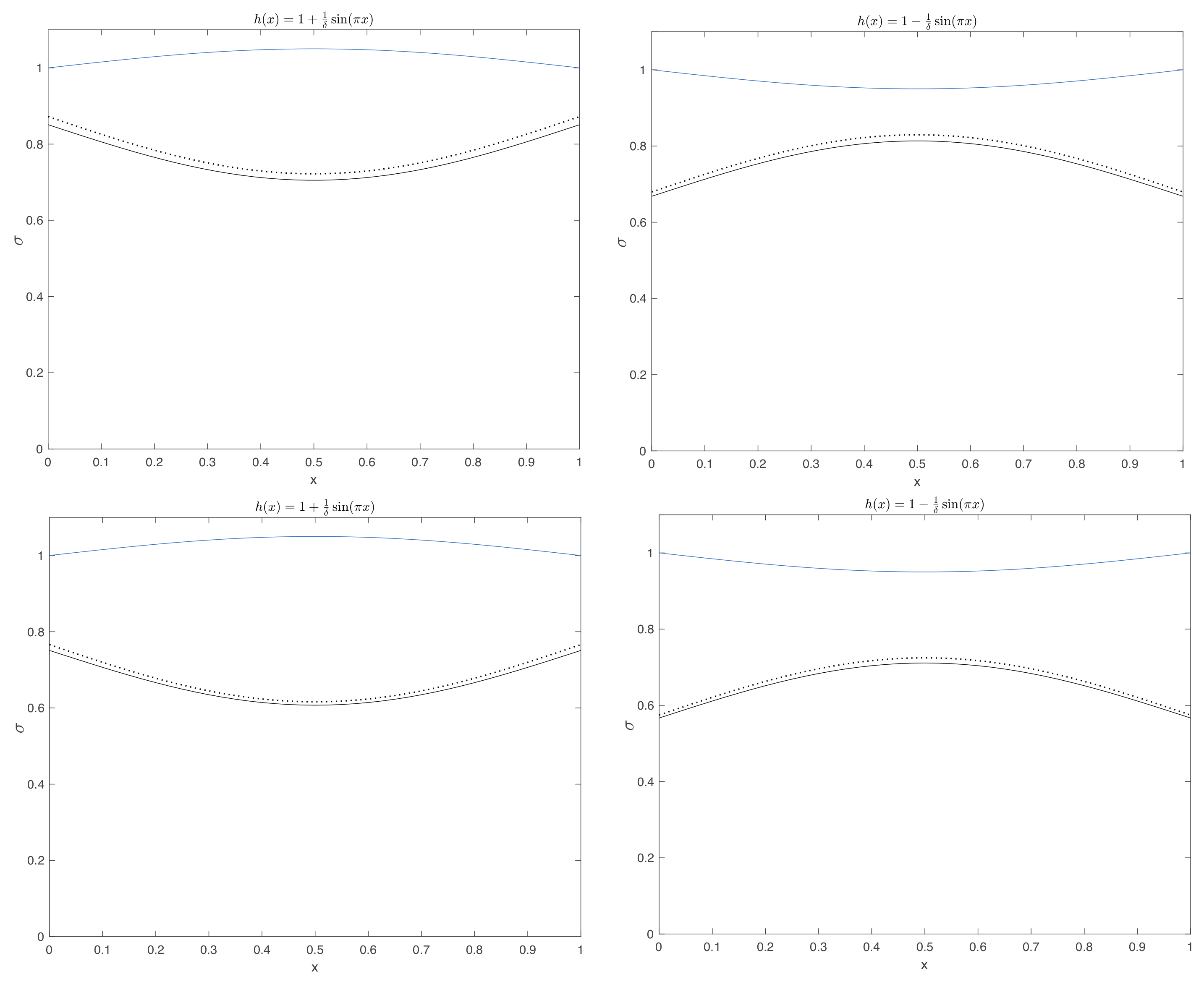
Figure 4 displays the yield surface when the wall profile is $h\left(x\right)=1\pm \frac{1}{\delta }sin\left(\pi x\right)$, with $\delta =20$, for various values of $B/\Delta p.$

The approximation here developed holds true for $|{\mathcal{P}}_x\left|\right|\sigma -h|<1$. So, to validate the procedure, we have to verify if $|{\mathcal{P}}_x\left|\right|\sigma -h|<1$ is fulfilled. Figure 5 shows the plot of $|{\mathcal{P}}_x\left|\right|\sigma -h|$ for the three cases displayed in Figure 4.

In the right panel of Figure 5, we notice that the condition under which the approximation is valid is not satisfied at the inlet and outlet.

In Figure 6, we report the comparison between $\sigma \left(x\right)$ given by (44) and $\sigma \left(x\right)$ obtained by the approximate model (55), (56). Figure 7 displays again the comparison between $\sigma \left(x\right)$ given by (44) and the approximated one, i.e., $\sigma \left(x\right)$ given by (55), (56), but now ${\displaystyle \frac{B}{\Delta p}}<{\displaystyle \frac{1}{2}}$, i.e., out of the range of validity of the approximate model. Figure 8 shows the comparison between $p\left(x\right)$ obtained solving (42), (43) and solving (56) when ${\displaystyle \frac{B}{\Delta p}}=0.75$, and ${\displaystyle \frac{B}{\Delta p}}=0.91$. Looking at Figure 7, one realizes that the two interfaces are quite similar, as in Figure 6, where $\frac{1}{2}<\frac{B}{\Delta p}<1$. On the other hand, the pressure profiles, displayed in Figure 8, are monotonously decreasing but show a different behavior, although we are in the range of the approximate model.

5.3. Comparison with the Pressure Driven Bingham Flow in a Channel

Problem (56) is similar to the one governing the Bingham flow in a channel, namely (see [12], Equation (39))

$$\left\{\begin{array}{c}{p}_{xx}+\left({\displaystyle \frac{6h_x\Delta p}{{\displaystyle 3h\Delta p+2\underset{0}{\overset{1}{\int }}{p}_{x}hdx-B}}}\right)p_x=0,\hfill \\ {\left.p\right|}_{x=0}=\Delta p,{\left.p\right|}_{x=1}=0,\hfill \end{array}\right.$$

(58)

with the yield surface given by (see again [12], Equation (34))

$$\sigma \left(x\right)=-2h\left(x\right))+\frac{B}{\Delta p}-\frac{2}{\Delta p}{\int }_0^1{p}_{x}hdx.$$

(59)

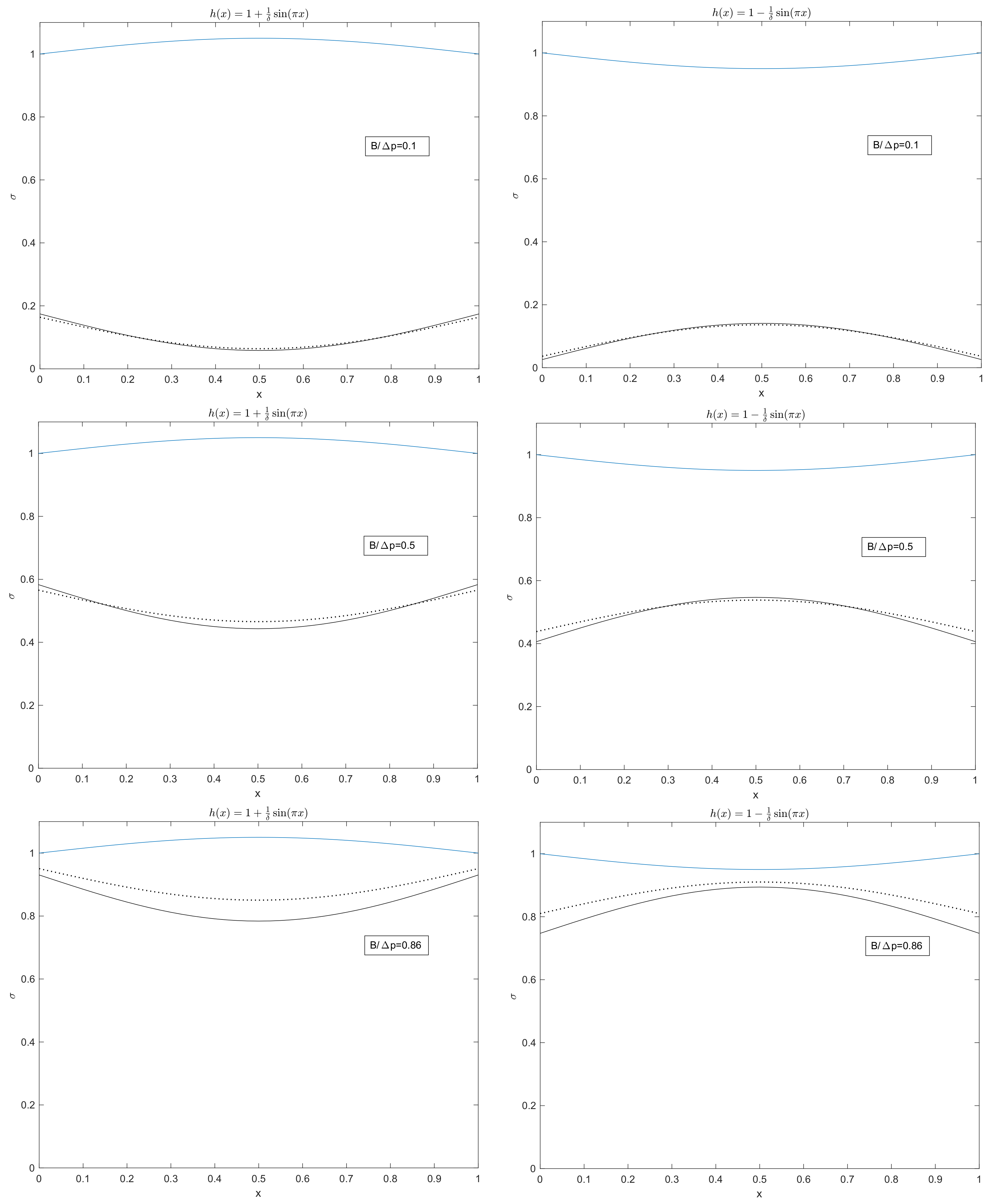
In Figure 9, we report the yield surface given by (59), i.e., the Bingham yield surface, and $\sigma \left(x\right)$ obtained solving (42) and (43), i.e., the Casson yield surface. We have considered three cases, $\frac{B}{\Delta p}=0.1$, 0.5 and 0.86.

The plots show that the two models give rise to similar curves when $\frac{B}{\Delta p}=0.1$ and 0.5. If $\frac{B}{\Delta p}=0.86$, the difference between the two curves is much more evident. We remark that, when $h\left(x\right)=1+\delta sin\left(\pi x\right)$, left panels, the largest difference occurs in the central region. On the contrary, when $h\left(x\right)=1-\delta sin\left(\pi x\right)$, right panels, the largest difference occurs in the external regions.

6. Peristaltic Flow

We now consider the case where the duct walls move as traveling waves, i.e., the peristaltic flow. We indeed assume that

$$h(x,t)=1+\frac{1}{\delta }sin\left(2\pi (x-t)\right),$$

(60)

that is a sinusoidal profile whose wave length and speed are equal to 1. Next, the boundary conditions of adhesion on $y=h$, i.e., (7), change and become

$$u(x,h,t)=0,v(x,h,t)=\frac{\partial h}{\partial t}.$$

Recalling (27) and following the same approach of Section 4, we have that

$$0=\frac{\partial Q(x,t)}{\partial x}=\frac{\partial }{\partial x}{\int }_0^{h\left(x,t\right)}udy\underset{{\left(14\right)}_1}{=}-\frac{\partial }{\partial x}{\int }_0^{h\left(x,t\right)}\frac{\partial v}{\partial y}dy,$$

which yields

$$\frac{\partial Q}{\partial x}=-\frac{\partial h}{\partial t}.$$

or, because of (60),

$$\frac{\partial }{\partial x}\left(Q-h\right)=0,$$

from which we conclude that $Q(x,t)-h(x,t)$ does not depend on x. Now, assuming that the inlet discharge $Q_{in}\left(t\right)=Q(0,t)$, we have

$$Q(x,t)-h(x,t)=Q_{in}\left(t\right)-h_{in}\left(t\right),$$

where $h_{in}\left(t\right)=h(0,t)$. Proceeding as in Section 5.2, we insert (52) in (27) and obtain

$$Q_{in}+h-h_{in}\left(t\right)=h{u}_c-{\displaystyle \frac{1}{12}}B{\mathcal{P}}_x^2{\displaystyle \frac{{(h-\sigma )}^4}{4}}=h{u}_c-u_c{\displaystyle \frac{(h-\sigma )}{4}}={\displaystyle \frac{u_c}{4}}\left(3h-\sigma \right).$$

(61)

Now, setting

$$\begin{array}{ccc}\hfill A\left(x,t\right)& =& Q_{in}\left(t\right)+h\left(x,t\right)-h_{in}\left(t\right)\hfill \\ & =& Q_{in}\left(t\right)+\frac{1}{\delta }\left[sin\left(2\pi \right(x-t\left)\right)+sin\left(2\pi t\right)\right],\hfill \end{array}$$

rearranging (61) yields

$$\sigma (x,t)={\displaystyle \frac{3h(x,t)u_c\left(t\right)-4A}{u_c\left(t\right)}},$$

(62)

with $u_c\left(t\right)$ still unknown at this stage. To determine the unknowns $\left(u_c,\sigma \right)$, we exploit (32)₂ and (61), obtaining this system

$$\left\{\begin{array}{c}\underset{0}{\overset{1}{{\displaystyle \int }}}{\mathcal{P}}_x\sigma dx=-1,\hfill \\ \sigma ={\displaystyle \frac{3h{u}_c-4A}{u_c}}.\hfill \end{array}\right.$$

(63)

To solve this problem, we exploit (52)₁ and (62) to determine ${\mathcal{P}}_x$ as a function of $u_c$. We thus have

$${\mathcal{P}}_x=-\sqrt{{\displaystyle \frac{12}{B}}}{\displaystyle \frac{u_c^2}{{(4A-2h{u}_c)}^{\frac{3}{2}}}},$$

(64)

where we choose the negative solution according to our assumption about $p_x$. Now, we put (64) in (63)₁, getting

$$\sqrt{{\displaystyle \frac{12}{B}}}{\int }_0^1{u}_c{\displaystyle \frac{3h{u}_c-4A}{{\left(4A-2h{u}_c\right)}^{\frac{3}{2}}}}dx=1,$$

(65)

with $u_c=u_c\left(t\right)$.

Simulations

To solve Equation (65), we have to impose some conditions on the integrand function. We require

$$\begin{array}{ccc}\hfill 4A-2h{u}_c& >& 0⟹{\displaystyle \frac{u_c}{A}}<{\displaystyle \frac{2}{h}},\hfill \\ \hfill 3h{u}_c-4A& >& 0⟹{\displaystyle \frac{u_c}{A}}>{\displaystyle \frac{4}{3h}},\hfill \end{array}$$

which, setting $\psi \left(x,t\right)={\displaystyle \frac{u_c\left(t\right)}{A\left(x,t\right)}}$, we rewrite as

$${\displaystyle \frac{4}{3h}}<\psi <{\displaystyle \frac{2}{h}}.$$

So, rearranging (65), we get

$$\sqrt{{\displaystyle \frac{12}{B}}}{\int }_0^1\sqrt{A}\psi {\displaystyle \frac{3h\psi -4}{{(4-2h\psi )}^{\frac{3}{2}}}}dx=1.$$

(66)

So, dividing the time interval $\left[0,1\right]$ in n steps, we solve numerically (66) at any time step. The results of simulations are displayed in Figure 10 and Figure 11.

7. Conclusions

In this paper, we have presented a mathematical model for a Casson flow in a symmetrical channel of varying amplitude whose walls can move over time as a traveling wave. The formulation of the fluid dynamics problem is obtained by imposing the mass and momentum balance. The latter, written for the central rigid core, results in an integral equation. We have thus determined an explicit expression for the velocity field and for the yield surface (which, being unknown, is a free boundary). The problem has been solved in two cases: (i) the driving force of the flow is the pressure difference applied between inlet and outlet; (ii) the inlet flow rate is imposed and the walls of the channel are animated by a traveling wave (peristaltic flow). Numerical simulations of the peristaltic flow have shown that as the Bingham number increases, and as the flow rate decreases, the yield surface tends to occupy the entire channel. Although an exhaustive parametric analysis has not been performed, the simulations carried out seem to show how the yield surface and channel walls oscillate in phase. This result (although not definitive) may have an important practical repercussion. Indeed, since $\sigma$ oscillates in phase with h, it is unlikely that the two surfaces touch and the flow stops. This fact, absent in the Bingham flows, could justify, if confirmed by further studies, the vasomotor action at the microcirculation level.

Regarding the analysis of the dynamics driven by the pressure gradient $\Delta p$, a comparison was made between the Bingham and the Casson flow. The results obtained seem to show a certain sensitivity to the $B/\Delta p$ parameter. Specifically, the two yield surfaces are similar when $B/\Delta p\sim 0.5$. As soon as $B/\Delta p$ tends to 0.9, the two surfaces detach significantly. In any case, we have found a well-known characteristic of viscoplastic flows in channels of variable amplitude: the yield surface and the channel wall have opposite monotonicity, that is, the plug shrinks (or widens) as the width of the channel increases (or decreases).