Abstract
We derive a new computational model for the simulation of viscous incompressible flows bounded by a thin, flexible, porous membrane. Our approach is grid-free and models the boundary forces with regularized Stokeslets. The flow across the porous membranes is modeled with regularized source doublets based on the notion that the flux velocity across the boundary can be viewed as the flow induced by a fluid source/sink pair with the sink on the high-pressure side of the boundary and magnitude proportional to the pressure difference across the membrane. Several validation examples are presented that illustrate how to calibrate the parameters in the model. We present an example consisting of flow in a closed domain that loses volume due to the fluid flux across the permeable boundary. We also present applications of the method to flow inside a channel of fixed geometry where sections of the boundary are permeable. The final example is a biological application of flow in a capillary with porous walls and a protein concentration advected and diffused in the fluid. In this case, the protein concentration modifies the pressure in the flow, producing dynamic changes to the flux across the walls. For this example, the proposed method is combined with finite differences for the concentration field.
1. Introduction
We present a new model for a type of problem in which a thin flexible porous boundary, such as a membrane, interacts with an incompressible viscous fluid. Problems of this nature arise in numerous biological applications such as in modeling cell membranes [1,2], microvasculature [3,4], and specialized anatomical structures such as the renal tubule [5,6,7]. Membranes are used in numerous medical applications such as drug delivery [2,8], biosensors [9,10] and tissue engineering [11]. Other more general engineering applications include membrane distillation processes [12], water filtration [8], and wastewater treatment [13]. There are widespread applications of microfiltration processes that take advantage of selective tuning of membrane permeability [14,15], and many theoretical and experimental investigations have focused on the swelling and permeability of gel dispersions in the microfluidic domain [16]. Theoretical studies have investigated the dynamics of particle interactions with deformable permeable membranes [17] as well as the behaviors of these membranes in complex flows [18].
There are numerical methods available for fluid flows bounded by a porous domain where the porous boundary does not deform [19,20]. Our goal is to address the case when an infinitely thin, flexible porous membrane divides the fluid domain. Some of the most closely related methods to our approach are described in [21,22]. Stockie [21] uses the immersed boundary method to model the Navier–Stokes equations with immersed elastic membranes and incorporates the porosity of the membrane by introducing a flux velocity across the boundary proportional to the hydrostatic pressure jump. A similar strategy is employed in [23] where the immersed boundary method and Darcy’s law are used to simulate the aerodynamics of a 2-D parachute, and in [24] to investigate effects of porosity on the motion of a flapping filament. Layton [22] uses a Cartesian grid method combined with Mayo’s technique [25], similar to the immersed interface method [26], to incorporate jump conditions into the finite-difference stencils. This formulation also incorporates a solute concentration into the model so that the flux velocity across the membrane can be a function of the hydrostatic pressure jump or the solute concentration differences across the boundary, a condition often encountered in biological settings. Using a coupled immersed boundary–lattice Boltzmann method, Pepona calculates fluid flow through and around a volumetric porous body that deforms elastically [27].
Exact solutions of Stokes flow through a permeable tube have been considered in several works. In particular, the seminal work of Berman [28] considered laminar Stokes flow near a porous boundary and has since been expanded to model flows in permeable cylinders [29,30,31]. These models assume low permeability and a small ratio between transverse and axial velocities. More recent studies have relaxed this assumption by deriving an exact solution for Stokes flow through a pipe of arbitrary permeability [19]. This work was later expanded to consider Stokes flow through a pipe of temporally dynamic radius to simulate “pumping” mechanisms encountered in numerous biological systems [20]. These analytical solutions assume that the position of the porous boundary is independent of the flow, as such they are useful for validation of numerical methods with a similar assumption.
Here, we present a grid-free method to model the motion of Stokes flows bounded by a flexible, elastic, porous membrane. The formulation of the model, as presented in the next section, applies to both two and three dimensions. The rest of the article focuses on the implementation and examples in two dimensions. The approach is based on the method of regularized Stokeslets, augmented with regularized source doublets on the porous boundaries. The latter is based on the notion that the flux velocity across the boundary can be considered as the flow induced by a fluid source/sink pair with the source on the high-pressure side of the boundary and magnitude proportional to the pressure difference across the membrane.
2. The Model Formulation
We consider a closed elastic membrane that encloses a two-dimensional domain . The membrane is given parametrically by where s is arc length, and is permeable to the fluid, whose motion is assumed to be described by the Stokes equations in . Since the membrane is elastic, it supports a force density given by . The equations of motion are
A fluid particle moves with velocity so that . Due to the permeability, the membrane moves with a different velocity field, namely , where is normal to the membrane and depends on the jump across the membrane of pressure or some other quantity.
2.1. A Different Formulation of the Problem
Given that the velocity of the fluid and the membrane differ by , we can write a general expression for the velocity field in the fluid domain including material points on the membrane as
where the last term on the right represents the membrane velocity. This term can also be interpreted as a velocity field whose divergence is . This leads to the formulation
2.2. The Proposed Regularized Formulation of the Problem
We use the linearity of the Stokes equations to separate the formulation in Equations (1)–(3) into two different problems whose solutions are added together. Let satisfy the incompressible Stokes equations with regularized external forcing
and let satisfy the Stokes equations without external forcing but with divergence given by a regularized source doublet distribution on the membrane
Then the fluid particles move with and the membrane moves with . The divergence of may be defined by the density function , where is the outward unit normal vector and is a coefficient that determines the membrane’s permeability, and is subject to the membrane properties.
Figure 1 shows a generic situation of the type considered in the next section. The figure shows the velocity field in a neighborhood of the membrane (top panel) as well as the divergence of the velocity (bottom panel) and the source doublet distribution that generates the flow. The bottom panel shows the vectors (black arrows) and the divergence of the velocity (colormap). The latter is negative just inside the membrane, indicating a distribution of sinks, and positive just outside, indicating a distribution of sources.
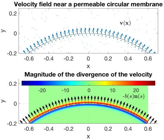
Figure 1.
General setting of the problems considered in this article. The figure shows a section of a circular permeable membrane. The top panel shows a neighborhood of the membrane and the velocity field across the membrane from the inside to the outside. This flow is generated by a distribution of source doublets on the membrane, with and is the outward unit normal. The bottom panel shows the vectors (black arrows) and the divergence of the velocity (colormap).
The function is used in the method of regularized Stokeslets [32,33] and is characterized by being smooth, radially symmetric functions concentrated at its center, like narrow Gaussians. The total integral is 1 and the parameter controls the spread of the function. In the formulation in (4) and (5), one could choose two different functions or use different values of even for the same function. In practice, the size of is influenced by the singularity of the corresponding singular kernel.
The solution of the problem in (4) is a regularized Stokeslet, given by [32,33]
where the regularized Green’s and biharmonic functions, and , corresponding to a radially symmetric blob are defined as the solutions of and in .
Derivation of the Source Doublet Solution
Take the divergence of the Stokes Equation (5) to get , and substitute the divergence expression from Equation (5), from which we find that the pressure is given by
Now the Stokes equation becomes
which leads to the velocity
For convenience we set , and summarize the solutions above as
where the regularizing functions are given by
2.3. Choice of Blobs
For a radially symmetric blob the minimum requirement is to have total integral equal to one
We use conditions derived in the first numerical example as part of the process of calibrating the source doublet coefficient . In all cases, we choose a blob and we use Equation (10) to find all necessary regularizing functions. Table 1 summarizes the blob functions used in this article.

Table 1.
Summary of regularizing functions. The blob satisfies only the condition that its integral be one. The function satisfies two more conditions for higher accuracy as described in example 1.
3. Numerical Examples
In order to assess the method, we present first two numerical examples whose exact solutions are known.
3.1. Example 1: A Circular Permeable Membrane under Tension
Consider a circular permeable membrane given initially by , where s is arclength. The force density is given by , where is curvature. The equations of motion are
Here, is a permeability parameter and represents the jump in pressure across the membrane, . The parameters in this example were assumed to be dimensionless and given by , and .
Exact solution. In this simple example, the membrane will remain circular for all times as it shrinks to a point in finite time. Due to incompressibility, the tension in the membrane serves to increase the pressure inside the circle but produces no fluid motion, so . The added membrane velocity is
where the pressure jump is computed from . Therefore . For a circular membrane, this reduces to an equation for its radius
with solution
Calibrating . The membrane velocity is normal to the membrane and is independent of position s along the membrane due to the circular symmetry. Thus, we compute it at , corresponding to . At this location, Equation (9) and give
Using the particular blob we find that
In order for this velocity to be consistent with the exact velocity in Equation (11), we choose
The coefficient depends on the blob used.
Based on the calculation of , we set and computed numerically the solution of the single differential equation with , corresponding to the blob . The solution using and is compared with the exact solution in Figure 2.
Figure 2.
Numerical solution of the ODEs for for the blobs (black) and (blue). The dashed curve is the exact solution of the problem. The left panel shows results for a constant regularization . The right panel shows results when the regularization size is varied dynamically according to .
Notice that the two curves in the figure are nearly indistinguishable until the circle has shrunk to a radius of about 0.1. Beyond this point, the blob size is equal to or larger than the radius of the circle and we do not expect the regularized velocity to approximate well the exact velocity. To ameliorate this issue we also computed the solution by scaling dynamically with the circle radius and reduced the error from a maximum of 0.078 to a maximum of 0.016.
We also computed the solution using a full simulation based on the velocity field
with . We discretized the initial circle using points equally spaced. The first and second derivatives of the membrane discretization with respect to the arc length parameter , are approximated by
where . They are used to approximate the outer normal vectors and curvature
For , we set , where . Using the notation and , the membrane points are evolved with the equation
The calibration method for allows for the introduction of two parameters and as unknown coefficients in the definition of the blob. We define a blob with integral equal to 1
Following the same calibration procedure as before leads to a version of Equation (12) of the form
and we select the parameters and to make and reduce the expression to
which leads to and the blob
We mention that Beale and collaborators [34,35] have derived conditions for regularized single and double layer potentials that increase the order of the regularization error. The conditions are that even moments of a certain function must be zero. Specifically, for each , the condition
increases the order of accuracy by two. Using these conditions (for and ) leads to the same two equations for and , so that the two procedures are equivalent.
The results are shown in Figure 3 using both blobs and the more accurate reducing the maximum error from 0.0827 to 0.0216 with fixed .
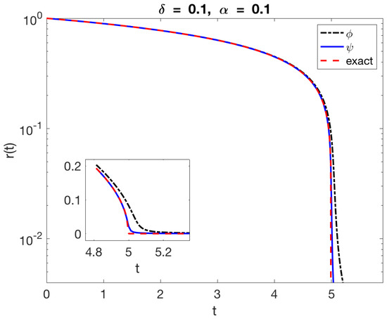
Figure 3.
Computation of the radius of the circle using the method in Equation (13) and the two blobs (dash-dot) and (solid) from Table 1. The dashed curve is the exact solution of the problem. The radius is shown in logarithmic scale to appreciate the difference between the solutions. The inset shows the results in linear scale near , when the exact solution shrinks to a point.
3.2. Example 2: A Circular Permeable Membrane with Circular Equilibrium
We consider the same circular membrane as in the previous example except that the force density along the membrane is given by , where is the equilibrium radius assumed to satisfy . In this case, the circle will shrink from initial radius to an asymptotic value of . The exact solution of the problem is given by [21]
and is the Lambert W-function. Using the parameter values , , and , we discretized the initial circle with N points , as before. The normal vectors, particle spacing and circle radius were computed as in the previous example so that the membrane motion is given by
where and . This system of equations is solved using a 4th order Runge–Kutta method and the blob in Table 1. The computed radius was compared to the exact solution resulting in the maximum errors shown in Table 2. The initial arc length parameter is computed as where and N is the number of membrane points. There are several observations we can make about the errors. Notice that the value of the regularization parameter is not constant in each column of the table since it depends on N. The errors for constant are along diagonals of the table; for example, the underlined values correspond to . With held constant, the errors decrease as decreases until the discretization error is small enough that the dominant error is due to the regularization (lower right corner of the table). If is chosen proportional to with sufficiently large proportionality constant (rightmost column of the table), the errors decrease by a factor of 4 as N doubles, indicating second-order convergence as expected from the choice in Equation (12). If is too small compared to , the errors reach a plateau (leftmost columns). The corresponding results using the blob in Table 1 are displayed in Table 3. Notice that the errors are smaller by several orders of magnitude.
Table 2.
Errors in the circle radius in example 2 using the blob . The errors were computed as . The initial arc length discretization is defined as . The underlined values correspond to errors for a fixed value of .
Table 3.
Errors in the circle radius in example 2 using the blob . The errors were computed as . The initial arc length discretization is defined as . The underlined values correspond to errors for a fixed value of .
Each row corresponds to a fixed discretization of the membrane and we see that for fixed N, as increases from to , the errors decrease to a minimum and eventually increase. The minimum values are smaller for finer discretizations (i.e., for larger N) and they occur at values of that are not the same multiple of . In other words, the errors decrease as both and are decreased but the optimal value of is not a fixed multiple of . This can be observed in Figure 4 left, which shows a log-log plot of the error versus . When is too small compared to , the errors are large since the blobs do not overlap sufficiently and fluid may leak between discretization nodes regardless of the value of . On the other hand, when is too large compared to , the regularization error is the largest contributor and the errors collapse onto a single line (in log-log scale) as long as the discretization is fine enough to approximate the smooth integral. Notice that the slope of the line corresponds to the sixth order leading error term in the value of found from the asymptotic expansion in Equation (14).
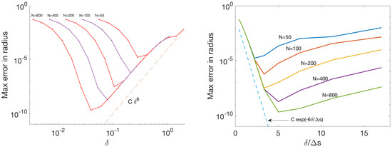
Figure 4.
Errors in the circle radius in example 2 using the blob . The (left) panel shows the errors plotted versus the discretization size . The (right) panel shows the errors plotted versus .
Figure 4 right shows the same errors except that they are plotted as a function of . In this scaling, the errors on the left side of the figure collapse onto a curve , indicating that in this example the discretization error decreases exponentially for the values tested when .
3.3. Example 3: Computing the Pressure
We consider an initially elliptical permeable membrane given by . As before, the force density is given by and the equations of motion are
The parameters used were , , and . The exact solution is unknown. The numerical solution at selected times is shown in Figure 5. Since the force density is proportional to the local curvature, the points along the major axis, where the curvature is largest, move in faster than other parts of the membrane. The two points along the minor axis move outward, changing the membrane’s shape into a more circular one. If the permeability is zero, no fluid can escape through the membrane and the membrane approaches a circle with area equal to the area bounded by the initial condition. When the permeability is nonzero, , fluid crosses the membrane as a function of the pressure drop across the boundary. This leads to an ever shrinking shape until it approaches a single point in finite time.
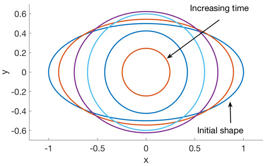
Figure 5.
Numerical solution of example 3 for the blob in Table 1 using permeability parameter , regularization parameter , , and = 1. The initial membrane shape was the ellipse of major axis 1 and minor axis 1/2. The figure shows the computed solution at times .
The computation proceeds as follows: for and , we compute the fluid velocity
using the discretization
with . The membrane velocity at is given by
where and . In this example, the formulas are derived for the blob from Table 1, where we used the value based on the calibration with this blob.
The pressure is given by
where when is inside the ellipse and 0 otherwise. A surface plot of the pressure, along with its cross-section in the -plane and contours in the -plane are shown in Figure 6.
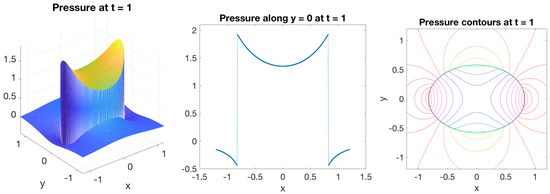
Figure 6.
Numerical solution of the pressure in example 3 at time for the blob in Table 1 using permeability parameter , regularization parameter , , and . The left panel shows the pressure in a region containing the membrane. The middle panel shows the pressure along the line . The right panel shows contours of the pressure.
3.4. Example 4: Flow in a Channel with Permeable Walls
We consider flow in a channel with walls that are permeable or have permeable sections, as depicted schematically in Figure 7. We assume that the flow at the inlet and at impermeable sections of the channel walls is given. The goal is to determine the flow within the channel for given boundary permeability. If the fluid velocity on the boundary of the channel were known, the flow in the channel could be computed using Stokeslets by solving for the boundary force. In the current case however, the fluid flow along the permeable boundary is unknown and satisfies , as in previous examples.
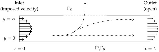
Figure 7.
Schematic of the channel. Parabolic flow given by for enters the channel at the left inlet. The height of the channel is and the length is . , the portion of the top wall within , is permeable and is represented by a dashed boundary; the rest of the top wall and the entire bottom wall () are solid. The right outlet is open. Dotted lines show potential fluid particle paths as the fluid interacts with the channel walls.
As a first step we use Stokeslets and source doublets to compute the velocity boundary condition in the permeable sections of the channel walls. Let represent the inlet, bottom and top sides of the channel, which constitute the boundary of the computational domain where forces are applied. Note that the channel outlet is not part of . Let be the permeable portion of , where , and set to be a parametrization of . We look for a force distribution on the channel walls along with a distribution of source doublets in the permeable region, with given, in order to determine the velocity on .
The procedure starts by setting on as
where is known at the inlet (parabolic) and along impermeable boundaries (zero). Setting and and using the following notation for the regularized Stokeslet and source doublet kernels
we enforce the boundary conditions
These are based on the assertion that the known boundary velocity is the sum of contributions from the Stokeslets and source doublets, while the unknown velocity across permeable channel walls is entirely due to the source doublets. The Stokeslets velocity contribution in those sections is zero.
Equation (19) must be inverted to find . Once the boundary force is known, the fluid velocity at the permeable boundary is set to . Now that all boundary velocities are known, the second step is to invert the Stokeslet kernel
to find and use it to compute the flow in the channel.
Figure 8 shows the result of the velocity boundary condition computation as well as the computed velocity near the outlet of the channel (right side) using the blob in Table 1. The figures are for three different values of while the inlet flow is the same in all cases. The viscosity was set to and the numerical parameters used were and wall discretization size . The figure shows that as increases, the permeability of the wall segment also increases, leading to more fluid escaping the channel at the top wall. When , more fluid escapes through the permeable wall than comes in through the inlet, leading to flow reversal at the right end of the channel. Figure 8 shows the velocity field in the channel computed from the Stokeslets that result from imposing the velocity boundary conditions. For , particles entering the channel at the inlet will flow to the outlet except those that are near the top wall. These get ejected out of the channel through the permeable top wall segment. The same is true for although particles in a larger region of the channel will flow out of the top. For , particles entering the channel at the inlet will necessarily flow out of the top permeable wall segment due to the flow reversal on the right side of the channel.
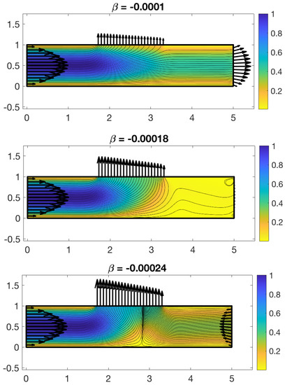
Figure 8.
Computed velocity boundary conditions (arrows) and velocity field streamlines for different values of . The colors represent the magnitude of the velocity in the channel. The numerical parameters used are and .
The flow rates shown in Table 4 were computed at the inlet, permeable wall, and outlet by a midpoint rule approximation of the integral
Table 4.
Computed flow rates at inlet, top wall, and outlet for different values of . The numerical parameters used are and .
Note that the exact flow rate at the inlet is .
3.5. Example 5: Flow in a Capillary with Protein Concentration
We consider a biological application of our formulation by modeling a single rat glomerular capillary using source doublets to represent pores in the membrane walls. The renal glomerulus is the structure responsible for filtering the blood in the kidney, and is composed of a tortuous network of over 300 capillary segments, wrapped into a sphere and surrounded by an outer capsule filled with the fluid filtrate from the capillaries [36]. Since this space is made up of fluid and not tissue, it is reasonable to model a glomerular capillary as a channel filled with and surrounded by fluid. Filtration in the glomerular capillaries is driven by a hydrostatic pressure [37]. The glomerular capillary walls are selectively permeable to fluid and solutes such as sodium and potassium, but impermeable to larger macromolecules including plasma proteins such as albumin. Due to the plasma protein concentration differential across the capillary wall between the blood plasma and filtrate, a colloid osmotic pressure, , is exerted in the direction of highest concentration, in this case back into the capillary and thus in opposition to . An expression for has been derived experimentally as a function of plasma protein concentration :
where is measured in g/dL and mmHg g dL, mmHg g dL [37]. Many 1-D models have been developed to estimate fluid filtration along the length of a glomerular capillary or the glomerulus as a whole [38,39,40,41,42]. Some computational fluid dynamics models have been developed to investigate glomerular filtration, including a model which used the immersed boundary method and finite element analysis to consider solute filtration in an idealized glomerulus in 3-D [43]. This study, while robust and detailed, did not consider the anatomy of the glomerulus and instead condensed the glomerulus into five cylinders that filtered in parallel. A 2-D model of fluid and solute filtration across a single portion of the glomerular membrane [44] studied intensely the sieving of solutes through the membrane, but did not consider the fluid dynamics within the capillary. To our knowledge the application of computational fluid dynamics to consider the dynamics of fluid filtration in an anatomically-accurate glomerular capillary in 2-D has not been performed.
To accomplish this task, we modify the previously-described channel algorithm (example 4) by introducing a concentration of plasma proteins that are transported by the fluid within the channel domain and cannot pass through the membrane:
with homogeneous Neumann conditions on the boundaries of the domain. At the inlet and outlet, the concentration is advected by the flow, so there is a need for an assumption on the concentration upstream of the inlet. We assume that is fixed at a high value so that plasma proteins are continuously introduced into the channel at the inlet.
To obtain the fluid velocity used to advect the concentration, we follow the algorithm outlined in example 4 with some modifications. Namely, the initial boundary flow must be modified to account for the influence of driving fluid back into the capillary and driving fluid out. is computed based on the concentration nearest to the permeable wall:
Assuming a constant along the length of the capillary [44] the effective filtration pressure difference across the channel walls is:
The resultant forces on the channel walls are solved for by inverting the source doublet kernel for the pressure:
Unlike previously described, this step assumes the constant as part of the formulation for pressure. This is because, in this case, the pressure-to-force relationship is independent of the membrane permeability. The constant is incorporated in the next step using the source doublet notation:
and we enforce the boundary conditions
The additional term on the right hand side of the equation is known, as such Equation (20) can be inverted to obtain and the boundary velocities in the permeable region are set to . The boundary velocities are known and the Stokeslet kernel is subsequently inverted for the forces which are used to find the channel fluid velocity. This velocity is then used to advect the plasma protein concentration. In Figure 9, we perform a temporal simulation in which an initial Gaussian concentration profile of protein (yellow circles in top left panel) is advected by the fluid while the fluid is filtered at the wall. As additional concentration is introduced at the inlet (yellow at the left wall in the bottom panels), the concentration develops local maxima at different locations in the channel. This simulation demonstrates the versatility of our method for predicting distribution of proteins throughout the vessel, as the protein concentration can vary with both time and location within the vessel. This is a significant improvement on previous models, which only consider axial changes in plasma protein concentration [38,39,40,41,42].
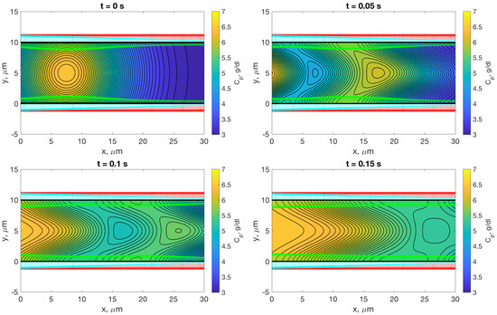
Figure 9.
Advection of concentration of plasma protein, , in a permeable channel with a constant velocity profile at the left boundary. Sources of concentration include an initial gaussian of concentration in the channel which is then added to by a constant protein concentration introduced at the left boundary. Red arrows indicate the velocity due to the hydrostatic pressure, , while green arrows indicate that due to the colloid osmotic pressure . Thus, these velocities are greatest where the concentration is largest, and change with the transport of the concentration. Cyan indicates the net flow due to both pressures in addition to the force exerted by the fluid moving with the velocity at the left boundary. The net velocity is scaled by 5 so as to be visible, when it is dwarfed in comparison to the velocities due to and . All three velocities are scaled by 2 for visibility.
The velocity at the inlet is defined as
where is chosen based on experimental data (Table 5). Parameters are chosen for the model based on measured dimensions of rat glomerular capillaries, red blood cell velocities and plasma viscosity [45].
Table 5.
Parameters for glomerular capillary simulations.
As explained in example 3, we use the blob , . In this example, by defining we use the same equation for and the dimensions of remain consistent. We calculate the fraction of filtered fluid to fluid entering the left end of the channel () by integrating the normal velocity through the permeable section of the membrane and dividing by the left velocity boundary condition:
Additional analysis elucidates a nonlinear relationship between the hydraulic conductivity k and the filtered fluid volume (Figure 10). This nonlinearity is transferred to the forces exerted on the wall in the normal and tangential directions (Figure 11). For forces in the tangential direction, a loss of fluid due to permeability reduces the force magnitude on the length of the vessel. The difference between these tangential stress profiles is nonlinear, corresponding to the nonlinear relationship between k and . For forces in the normal direction, a linear drop in force across the vessel is seen for all values of k. This is expected due to the necessary pressure drop across the vessel to facilitate the flow imposed at the left boundary. However with increasing k the force in the normal direction is reduced nonlinearly, corresponding to the nonlinear relationship between k and .
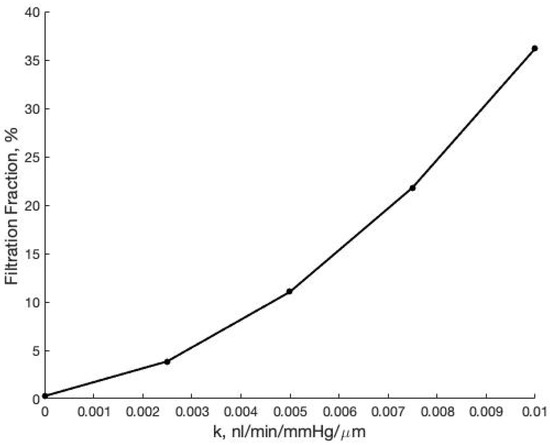
Figure 10.
Filtration fraction, as a function of the hydraulic conductivity k of the vessel wall which ultimately dictates the value of .
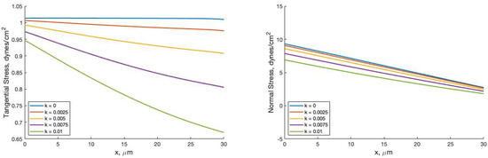
Figure 11.
Tangential forces (left) and normal forces (right) on the vessel length for varied values of hydraulic conductivity k.
Inherent to our current application of Stokeslets and source doublets to compute the fluid dynamics within a permeable glomerular capillary is the assumption that the walls are not deflected by flow through the capillary such that the capillary diameter remains constant in time. In reality, the glomerular capillary walls change in time due to the pulsatility of blood pressure. We have previously estimated the magnitude of strain of the glomerular capillary walls using a mathematical model of blood flow through an entire anatomically accurate glomerular capillary network [48], and found that the magnitude of glomerular capillary wall strain is, under physiological conditions, less than 1%. Future models will investigate dynamics of adding flexibility to the vessel wall as well as changing the diameter of the vessel as a function of length.
4. Discussion and Conclusions
We have presented a model for computing flows bounded by thin permeable membranes in which the amount of fluid that is filtrated across the membrane depends on local flow properties such as the pressure drop across the membrane, the concentration of a solute, and the membrane permeability.
The derivation was based on the concept of placing fluid sources on one side of the membrane and corresponding sinks on the other side, creating a source doublet field along the permeable parts of the membrane. We note that the resulting source doublet kernel is the same as that of a flow proportional to the pressure gradient due to a force normal to the boundary. Indeed, decomposing a force into a gradient and a zero-divergence vector field gives
The kernel in Equation (9) is the same as this expression for .
Our model builds on the method of regularized Stokeslets through the use of regularized sources. The resulting boundary integral formulation is free of singularities and the regularization parameter provides a length scale for the thickness of the membrane. In addition, the strength of the source doublet is proportional to the regularization parameter with proportionality constant that depends on the used. Our numerical results demonstrate that designing the regularization function to satisfy the moment condition in Equation (15) [34,35] leads to higher accuracy, in practice.
The last two examples present applications to channel flow. Example 4 involves a channel with only a section of the boundary that is permeable to the fluid, while the velocity field at the Inlet is assumed to be given and the no slip condition is enforced in the impermeable portions of the boundary, the velocity boundary condition is unknown in the permeable section, and therefore, unknown also at the outlet. We use the model proposed here specifically to determine the velocity boundary condition at the permeable section of the channel in a way that is consistent with the normal stress along the boundary. Once this is known, the flow in the channel is computed using the method of regularized Stokeslets. The example shows that if the permeability is high enough, more fluid escapes through the permeable membrane than fluid comes in through the inlet, forcing fluid into the channel at the outlet. The final example provides an application in which a concentration flows and diffuses in the channel, whose walls are permeable to the fluid but not to , and the concentration level affects the permeability locally.
There are extensions to this model that we expect to pursue in the future. Each wall of the channel can be treated as a set of connected linear segments with a force density that varies linearly on each segment. Then the integral in Equations (6) and (9) can be computed analytically, as explained in [49]. This would allow the use of substantially smaller values of the regularization without increasing (in fact, decreasing) the number of nodes discretizing the boundary. Finally, we note that our boundary integral model describing the flow across a permeable membrane is valid in three dimensions as well, so that extending the method to 3D is straight forward.
Author Contributions
Conceptualization, R.C. and M.H.-V.; methodology, R.C.; software, R.C., M.H.-V. and O.R.; formal analysis, R.C., M.H.-V. and O.R.; writing—original draft preparation, R.C. and M.H.-V.; writing—review and editing, R.C. and O.R.; visualization, R.C., M.H.-V. and O.R.; supervision, R.C.; project administration, R.C. All authors have read and agreed to the published version of the manuscript.
Funding
At the time this study was conducted, O.R. was a graduate student in the Tulane University Bioinnovation Program, supported by NSF IGERT Grant NSF DGE-1144646. O.R. received additional funding from the NIH fellowship grant NIH F31 DK121445.
Conflicts of Interest
The authors declare no conflict of interest. The funders had no role in the design of the study; in the collection, analyses, or interpretation of data; in the writing of the manuscript, or in the decision to publish the results.
References
- Stillwell, W.; Ehringer, W.; Jenski, L.J. Docosahexaenoic acid increases permeability of lipid vesicles and tumor cells. Lipids 1993, 28, 103–108. [Google Scholar] [CrossRef] [PubMed]
- Yang, N.J.; Hinner, M.J. Getting across the cell membrane: An overview for small molecules, peptides, and proteins. Methods Mol. Biol. 2015, 1266, 29–53. [Google Scholar] [CrossRef] [PubMed]
- Michel, C.; Curry, F. Microvascular permeability. Physiol. Rev. 1999, 79, 703–761. [Google Scholar] [CrossRef] [PubMed]
- Nagy, J.A.; Benjamin, L.; Zeng, H.; Dvorak, A.M.; Dvorak, H.F. Vascular permeability, vascular hyperpermeability and angiogenesis. Angiogenesis 2008, 11, 109–119. [Google Scholar] [CrossRef] [PubMed]
- Pennell, J.P.; Lacy, F.B.; Jamison, R.L. An in vivo study of the concentrating process in the descending limb of Henle’s loop. Kidney Int. 1974, 5, 337–347. [Google Scholar] [CrossRef] [PubMed]
- Knepper, M.A.; Danielson, R.A.; Saidel, G.M.; Post, R.S. Quantitative analysis of renal medullary anatomy in rats and rabbits. Kidney Int. 1977, 12, 313–323. [Google Scholar] [CrossRef] [PubMed]
- Layton, A.T. Mathematical modeling of kidney transport. Wiley Interdiscip. Rev. Syst. Biol. Med. 2013, 5, 557–573. [Google Scholar] [CrossRef]
- Jackson, E.A.; Hillmyer, M.A. Nanoporous membranes derived from block copolymers: From drug delivery to water filtration. ACS Nano 2010, 4, 3548–3553. [Google Scholar] [CrossRef]
- Baronas, R.; Ivanauskas, F.; Kaunietis, I.; Laurinavicius, V. Mathematical Modeling of Plate- gap Biosensors with an Outer Porous Membrane. Sensors 2006, 6, 727–745. [Google Scholar] [CrossRef]
- Hurk, R.v.d.; Evoy, S. A review of membrane-based biosensors for pathogen detection. Sensors 2015, 15, 14045–14078. [Google Scholar] [CrossRef]
- Stamatialis, D.F.; Papenburg, B.J.; Girones, M.; Saiful, S.; Bettahalli, S.N.; Schmitmeier, S.; Wessling, M. Medical applications of membranes: Drug delivery, artificial organs and tissue engineering. J. Membr. Sci. 2008, 308, 1–34. [Google Scholar] [CrossRef]
- Ugrozov, V.V.; Elkina, I.B. Mathematical modeling of influence of porous structure a membrane on its vapour-conductivity in the process of membrane distillation. Desalination 2002, 147, 167–171. [Google Scholar] [CrossRef]
- Yun, M.A.; Yeon, K.M.; Park, J.S.; Lee, C.H.; Chun, J.; Lim, D.J. Characterization of biofilm structure and its effect on membrane permeability in MBR for dye wastewater treatment. Water Res. 2006, 40, 45–52. [Google Scholar] [CrossRef] [PubMed]
- Kim, W.K.; Kanduč, M.; Roa, R.; Dzubiella, J. Tuning the Permeability of Dense Membranes by Shaping Nanoscale Potentials. Phys. Rev. Lett. 2019, 122, 108001. [Google Scholar] [CrossRef]
- Kim, W.K.; Chudoba, R.; Milster, S.; Roa, R.; Kanduč, M.; Dzubiella, J. Tuning the selective permeability of polydisperse polymer networks. Soft Matter 2020, 16, 8144–8154. [Google Scholar] [CrossRef]
- Holmqvist, P.; Mohanty, P.S.; Nägele, G.; Schurtenberger, P.; Heinen, M. Structure and Dynamics of Loosely Cross-Linked Ionic Microgel Dispersions in the Fluid Regime. Phys. Rev. Lett. 2012, 109, 048302. [Google Scholar] [CrossRef] [PubMed]
- Daddi-Moussa-Ider, A.; Gekle, S. Brownian motion near an elastic cell membrane: A theoretical study. Eur. Phys. J. E 2018, 41, 19. [Google Scholar] [CrossRef]
- Bächer, C.; Gekle, S. Computational modeling of active deformable membranes embedded in three-dimensional flows. Phys. Rev. E 2019, 99, 062418. [Google Scholar] [CrossRef]
- Herschlag, G.; Liu, J.G.; Layton, A.T. An Exact Solution for Stokes Flow in a Channel with Arbitrarily Large Wall Permeability. SIAM J. Appl. Math. 2014, 75, 2246–2267. [Google Scholar] [CrossRef]
- Herschlag, G.; Liu, J.G.; Layton, A. Fluid extraction across pumping and permeable walls in the viscous limit. Phys. Fluids 2016, 28, 041902. [Google Scholar] [CrossRef]
- Stockie, J.M. Modelling and simulation of porous immersed boundaries. Comput. Struct. 2009, 87, 701–709. [Google Scholar] [CrossRef]
- Layton, A.T. Modeling Water Transport across Elastic Boundaries Using an Explicit Jump Method. SIAM J. Sci. Comput. 2006, 28, 2189–2207. [Google Scholar] [CrossRef]
- Kim, Y.; Peskin, C. 2–D Parachute Simulation by the Immersed Boundary Method. SIAM J. Sci. Comput. 2006, 28, 2294–2312. [Google Scholar] [CrossRef]
- Natali, D.; Pralits, J.O.; Mazzino, A.; Bagheri, S. Stabilizing effect of porosity on a flapping filament. J. Fluids Struct. 2016, 61, 362–375. [Google Scholar] [CrossRef]
- Mayo, A. The fast solution of Poisson’s and the biharmonic equations on irregular regions. SIAM J. Numer. Anal. 1984, 21, 285–299. [Google Scholar] [CrossRef]
- LeVeque, R.J.; Li, Z. The Immersed Interface Method for Elliptic Equations With Discontinuous Coefficients and Singular Sources. SIAM J. Numer. Anal. 1992, 31, 332–364. [Google Scholar]
- Pepona, M.; Favier, J. A coupled Immersed Boundary–Lattice Boltzmann method for incompressible flows through moving porous media. J. Comput. Phys. 2016, 321, 1170–1184. [Google Scholar] [CrossRef]
- Berman, A.S. Laminar flow in channels with porous walls. J. Appl. Phys. 1953, 24, 1232–1235. [Google Scholar] [CrossRef]
- Yuan, S. Laminar Pipe Flow with Injection and Suction through a Porous Wall; Technical Report; James Forrestal Research Center, Princeton University: Princeton, NJ, USA, 1955. [Google Scholar]
- Wah, T. Laminar flow in a uniformly porous channel. Aeronaut. Q. 1964, 15, 299–310. [Google Scholar] [CrossRef]
- Terrill, R.M.; Shrestha, G.M. Laminar flow through parallel and uniformly porous walls of different permeability. Z. Angew. Math. Phys. ZAMP 1965, 16, 470–482. [Google Scholar] [CrossRef]
- Cortez, R. The method of regularized Stokeslets. SIAM J. Sci. Comput. 2001, 23, 1204–1225. [Google Scholar] [CrossRef]
- Cortez, R.; Fauci, L.; Medovikov, A. The method of regularized Stokeslets in Three Dimensions: Analysis, Validation and Application to Helical Swimming. Phys. Fluids 2005, 17, 031504. [Google Scholar] [CrossRef]
- Beale, J.T. A Convergent Boundary Integral Method for Three-Dimensional Water Waves. Math. Comput. 2001, 70, 977–1029. [Google Scholar] [CrossRef]
- Tlupova, S.; Beale, J.T. Regularized single and double layer integrals in 3D Stokes flow. J. Comput. Phys. 2019, 386, 568–584. [Google Scholar] [CrossRef]
- Shea, S.M. Glomerular hemodynamics and vascular structure: The pattern and dimensions of a single rat glomerular capillary network reconstructed from ultrathin sections. Microvasc. Res. 1979, 18, 129–143. [Google Scholar] [CrossRef]
- Arendshorst, W.; Navar, L. Renal circulation and glomerular hemodynamics. In Diseases of the Kidney, 8th ed.; Schrier, R., Ed.; Walters Kluwer/Lippincott Williams and Wilkins: Philadelphia, PA, USA, 2007; Chapter 2; Volume 1, pp. 54–95. [Google Scholar]
- Deen, W.; Robertson, C.; Brenner, B. A model of glomerular ultrafiltration in the rat. Am. J. Physiol.-Leg. Content 1972, 223, 1178–1183. [Google Scholar] [CrossRef] [PubMed]
- Deen, W.M.; Bohrer, M.P.; Brenner, B.M. Macromolecule transport across glomerular capillaries: Application of pore theory. Kidney Int. 1979, 16, 353–365. [Google Scholar] [CrossRef]
- Deen, W.M.; Lazzara, M.J.; Myers, B.D. Structural determinants of glomerular permeability. Am. J. Physiol.-Ren. Physiol. 2001, 281, F579–F596. [Google Scholar] [CrossRef]
- Lambert, P.; Aeikens, B.; Bohle, A.; Hanus, F.; Pegoff, S.; Van Damme, M. A network model of glomerular function. Microvasc. Res. 1982, 23, 99–128. [Google Scholar] [CrossRef]
- Remuzzi, A.; Brenner, B.M.; Pata, V.; Tebaldi, G.; Mariano, R.; Belloro, A.; Remuzzi, G. Three-dimensional reconstructed glomerular capillary network: Blood flow distribution and local filtration. Am. J. Physiol.-Ren. Physiol. 1992, 263, F562–F572. [Google Scholar] [CrossRef]
- de Sousa, D.; Ferreira, M.C. Ultrafiltration in Renal Glomerular Capillaries: Theoretical Effects of Ultrastructure. Ph.D. Thesis, Massachusetts Institute of Technology, Cambridge, MA, USA, 1994. [Google Scholar]
- Layton, A.T.; Edwards, A. Glomerular Filtration. In Mathematical Modeling in Renal Physiology; Springer: Berlin/Heidelberg, Germany, 2014; pp. 7–41. [Google Scholar]
- Ferrell, N.; Sandoval, R.M.; Bian, A.; Campos-Bilderback, S.B.; Molitoris, B.A.; Fissell, W.H. Shear stress is normalized in glomerular capillaries following 5/6 nephrectomy. Am. J. Physiol.-Ren. Physiol. 2015, 308, F588–F593. [Google Scholar] [CrossRef]
- Wakeham, W.; Salpadoru, N.; Caro, C. Diffusion coefficients for protein molecules in blood serum. Atherosclerosis 1976, 25, 225–235. [Google Scholar] [CrossRef]
- Zatz, R.; Dunn, B.R.; Meyer, T.W.; Anderson, S.; Rennke, H.G.; Brenner, B.M. Prevention of diabetic glomerulopathy by pharmacological amelioration of glomerular capillary hypertension. J. Clin. Investig. 1986, 77, 1925–1930. [Google Scholar] [CrossRef] [PubMed]
- Richfield, O.; Cortez, R.; Navar, L.G. Simulations of increased glomerular capillary wall strain in the 5/6-nephrectomized rat. Microcirculation 2021, 28, e12721. [Google Scholar] [CrossRef] [PubMed]
- Cortez, R. Regularized Stokeslet segments. J. Comput. Phys. 2018, 375, 783–796. [Google Scholar] [CrossRef]


Publisher’s Note: MDPI stays neutral with regard to jurisdictional claims in published maps and institutional affiliations. |
© 2021 by the authors. Licensee MDPI, Basel, Switzerland. This article is an open access article distributed under the terms and conditions of the Creative Commons Attribution (CC BY) license (https://creativecommons.org/licenses/by/4.0/).