2.1. Compressible Blasius Equations
Incompressible Blasius solution is a similarity solution for a flat plate. The assumptions for the incompressible Blasius equations are given in our previous work [
19]; interested readers can check the details from there. In the compressible region, the temperature effects must be taken into account for an accurate solution. In the incompressible region, the temperature and density changes are small enough to be neglected. In the compressible region, the temperature can increase drastically as a result; density decreases within the boundary-layer. For example, the temperature on the solid wall can reach 7 times the freestream temperature in Mach 6 flow over a wedge. If the freestream temperature is 300 K, the wall temperature will be around 2100 K. In order to compare the quantity, the melting point of titanium is around 1941 K [
45]. This problem is still a challenge for aerospace applications in which high Mach numbers are involved.
The compressible Blasius equations can be derived from the compressible Navier–Stokes equations, which can be expressed in two spatial dimensions as:
where
is the density,
u and
v are the velocities in
x- and
y- directions,
p is the pressure,
is the dynamic viscosity,
is the second viscosity coefficient,
k is the thermal conductivity,
T is the temperature,
is the specific heat at constant pressure, and
is the dissipation function, which can be written as:
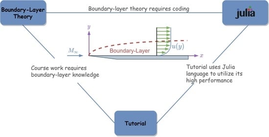
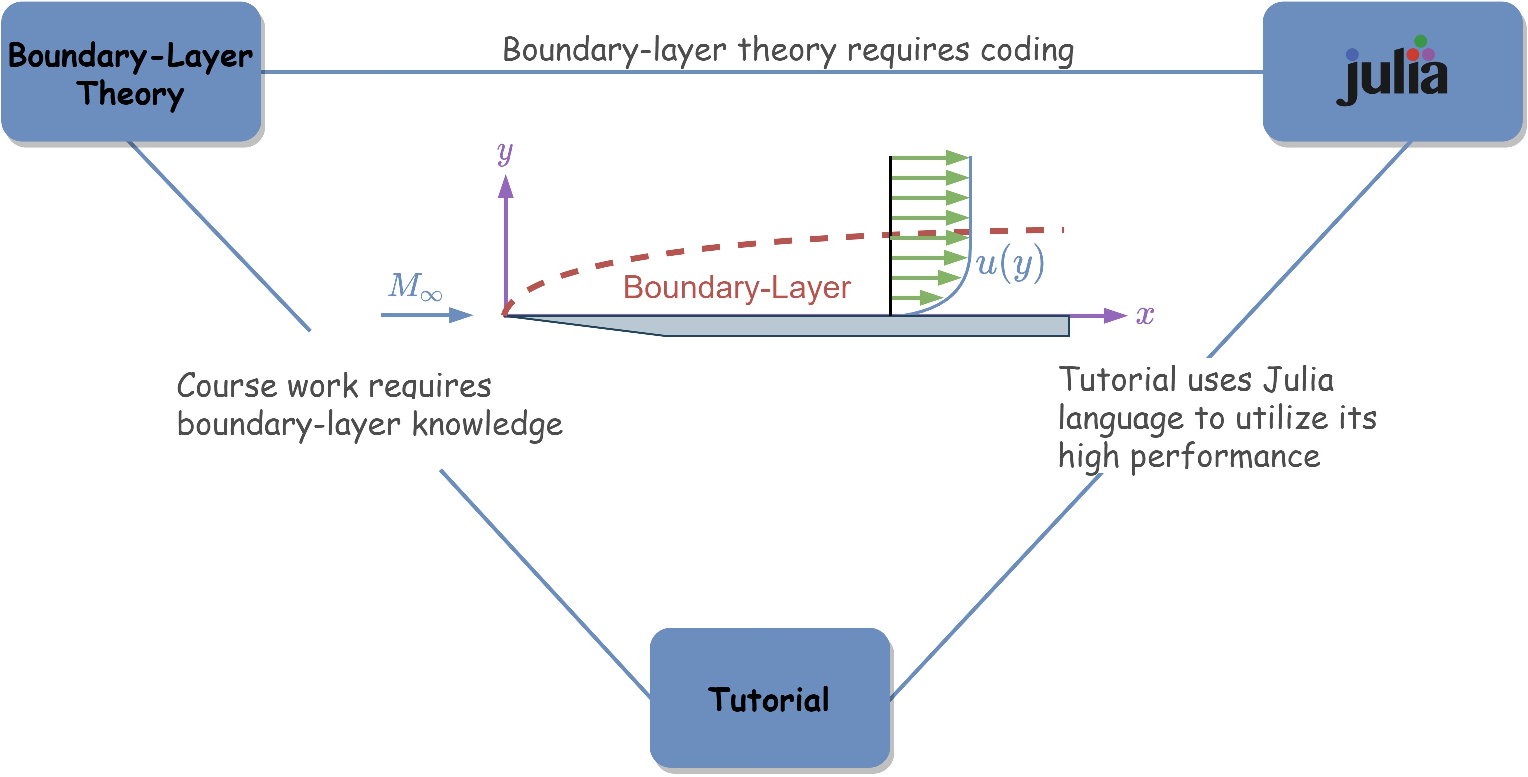
In order to obtain the boundary-layer equations, dimensional analysis is required to neglect the variables that have smaller orders than others. The flat plate boundary-layer development is illustrated in
Figure 2. In this flow,
u velocity is related to freestream velocity and the order of magnitude is one. The
x is related to plate length, so its order of magnitude is also one. The
y distance is related to boundary-layer thickness, so it is in the order of
which is the boundary-layer thickness. The density,
, is related to freestream density so its order of magnitude is also one. The magnitude of the
v velocity can be calculated from the continuity equation, Equation (
1). In order to get zero from this equation, all variables must be in the same order so
v is in the order of
as a result of this,
. When the magnitude analysis is completed in the same manner, the boundary-layer equations can be obtained. It has to be noted that dynamic viscosity is in the order of
, pressure and temperature are in the order of one. The specific heat at constant pressure is in the order of one. The second viscosity coefficient,
, can be taken as
because of Stokes’ hypothesis. Once the order of magnitude is obtained for each of the terms, some of the terms can be neglected because
. The final system of equations in steady-state condition (
) will be:
Equation (7) can be expressed at the boundary-layer edge as:
The variables are changing from the solid surface up to the boundary-layer edge. At the boundary-layer edge, they reach to freestream value for the corresponding variable and remain constant. The velocity change in the
y-direction at the boundary-layer edge is zero (
), because it is constant at boundary-layer edge. Equation (8) indicates that the pressure gradient in the
y-direction is zero, so pressure at the boundary-layer edge equals the pressure within the boundary-layer (
). Equation (
10) becomes:
The velocity at the boundary-layer edge is equal to freestream velocity, which is constant in
x-direction for a flat plate. In other words, edge velocity gradient in
x-direction is zero (
). If the equation of state is used to obtain the ratio of density and temperature as:
where
R is the gas constant. It is known that
, so
. The final system of equations is:
where
. At this point, a similarity parameter can be introduced to the system to obtain a similarity solution [
46]. The similarity parameter,
, can be defined as:
where
. Let’s assume that the stream function is
The
u and
v velocities can be calculated from the stream function as:
In this step, the variables in Equation (15),
u,
v,
,
, and
can be calculated. The first derivative of
with respect to
y and the first derivative of
s with respect to
x will be required for the chain rule.
It is better to note that, in
calculation,
relation is used. The
u velocity can be calculated as:
The same procedure can be applied for
v velocity as:
Once
u velocity is obtained, the derivatives with respect to
x and
y can be calculated as:
All terms in Equation (15) are known. If the above terms are substituted into Equation (15) and the necessary simplifications are done, the final equation will be:
It has to be noted that if
and
, in other words, if the flow is incompressible, Equation (
41) becomes an incompressible Blasius equation (
). Equation (
41) can be further simplified as:
where
and
. The momentum equation of the compressible Blasius equations is obtained in Equation (
42). The energy equation of the compressible Blasius equations can be obtained with the same procedure. First of all,
,
, and
have to be calculated. These terms can be calculated as:
When these terms are substituted into Equation (17), the new equation will be:
Equation (
51) can be simplified by dividing it with
, substituting Prandtl number into the equation where Prandtl number
and multiplying with
. The final equation will be:
where
,
, and
. In the final system of equations, the
can be calculated from Sutherland Viscosity Law [
47]. The dimensional viscosity function is:
where
and
K. The
is:
The derivative of the viscosity is also required. The derivative terms can be calculated as:
The final system of equations is:
It has to be emphasized that
is a function of
and the final system of equations is coupled, so they have to be solved together. The boundary conditions of the system for an adiabatic system are:
The boundary condition for the isothermal wall depends on the wall temperature. For example, if the wall temperature equals the boundary-layer edge temperature, it will be , and it will be replaced with the last boundary condition of the system. In the adiabatic boundary condition, the derivative of the temperature with respect to wall-normal direction will be 0. During the numerical procedures, the difference will be emphasized one more time.
2.2. Numerical Procedure
In this section, the compressible Blasius equation will be solved with the fourth-order Runge–Kutta method [
48] and Newton’s iteration method [
49]. Different methods can be used for this problem; however, we used Runge–Kutta and Newton’s method because of their extensive usage in the literature and accuracy. To start the numerical procedure, high-order differential equations can be reduced to the first-order differential equations as:
if Equations (
64)–(68) are substituted into Equations (
58) and (59), the final version of these equations can be written as:
The final system of equations can be written in the matrix form as:
The adiabatic boundary conditions for the system are:
The isothermal boundary conditions for the system are:
The functions can be introduced in Julia as shown in Listing 1, where
is the second coefficient of the Sutherland Viscosity Law,
is the temperature at the boundary-layer edge,
is the Mach number at the boundary-layer edge,
is the specific heat ratio,
is the Prandtl number and
and
are the terms given in Equations (
64)–(66), Equation (67), and Equation (68). In the functions given in Listing 1, only 2 parameters are dimensional, which are
and
. In this tutorial paper, Kelvin is the unit of both parameters. If the temperature unit is required to be different, such as Fahrenheit or Rankine, the units of
and
must be transformed into the new unit accordingly.
Listing 1.
Implementation of system of equations in Julia environment. There are five functions which correspond to five first-order ordinary differential equations.
Listing 1.
Implementation of system of equations in Julia environment. There are five functions which correspond to five first-order ordinary differential equations.
In this paper, implementation of the Runge–Kutta method will be provided. The derivation of the Runge–Kutta method and how it calculates the function value at the next step can be checked from Reference [
49]. The implementation of the Runge–Kutta method for the compressible Blasius problem can be seen in Listing 2, where
N is the number of elements. It has to be emphasized that the number of node points is
, which means that terms must be calculated until
node. The first point is the boundary condition, so there will be
N number of calculations.
The initialization and the boundary conditions can be introduced as shown in Listing 3, where is a flag for the adiabatic or isothermal condition selection and is the dimensionless wall temperature. It is nondimensionalized with , so if the temperature at the boundary-layer edge, , is 300 K and the wall temperature is required to be 150 K, must be entered as . Another important point about Listing 3 is the indices. In the derived formulations, indices start from 0. However, in both Julia and MATLAB, indices start from 1. This is the reason why indices are starting from 1 in Listing 3 boundary conditions part.
Listing 2.
Implementation of Runge-Kutta method in Julia environment. It requires four slope calculation to estimate the function value in the next node value.
Listing 2.
Implementation of Runge-Kutta method in Julia environment. It requires four slope calculation to estimate the function value in the next node value.
In the system of equations, there are five equations and five boundary conditions; however, two boundary conditions are located at the end of the domain. In order to start the calculation, all values at the
should be given.
and
in the Listing 3 are the initial guesses for the missing boundary conditions. They can be any value. Once they are introduced to the system, compressible Blasius equations can be solved. When the equations are solved with guessed initial conditions, the solution vector must satisfy the boundary conditions at the end of the domain. However, it will not converge at the first try because the guessed boundary conditions are not correct. To overcome this problem, different methods can be used, such as the shooting method, bisection method, or Newton’s iteration method. In this paper, Newton’s iteration method will be used because it is fast and it is not hard to implement. In order to use it, the algorithm needs to run with the initial guesses one time. Once the
(corresponds to
u) and
(corresponds to
T) at the end of the domain are obtained, an arbitrary small number can be added to one of the initial guesses. The algorithm can be run one more time with the new boundary condition guesses. After that, the same small number can be added to the other initial guess and the algorithm can be run one more time. After running the algorithm 3 times, there will be 3 different
–
pairs. It has to be noted that when the small number is added to the second boundary condition (in the third run), other boundary conditions should be equal to the value in the first run. In other words, after adding a small value in the second run, it should be subtracted in the third run. The main purpose of running three times is to determine the more accurate boundary condition guess. The new boundary conditions can be calculated with:
where
and
are the initially guessed boundary conditions.
and
are required for the new boundary conditions. These values can be approximated from the Taylor series expansion of the
and
, which can be shown as:
and
must be 1 due to the boundary conditions. The new system of equations for the
and
will be:
The partial differentials can be approximated with the finite difference as:
where
and
are the values obtained from the first run,
and
are the values obtained from the second run, and
and
are the values obtained from the third run. Once everything is calculated, the system of equations in Equation (
86) can be used to calculate
and
. The implementation of the explained method in Julia can be seen in Listing 4.
Listing 3.
Initialization of the variables and implementation of boundary conditions in Julia environment. The boundary conditions for adiabatic and isothermal conditions are different than each other.
Listing 3.
Initialization of the variables and implementation of boundary conditions in Julia environment. The boundary conditions for adiabatic and isothermal conditions are different than each other.
The same procedure will run until
, and
at the end of the domain will be 1. It is important to decide the upper limit of the domain. If it is small, it will force the value at that point to be 1 where it should not be. It is also important to choose the small number,
, smaller than convergence criteria which will finalize the simulation. If
is higher than the convergence criteria, the simulation might run until it reaches the maximum iteration number. In the code provided in GitHub, convergence criteria is taken as
and the small number is taken as
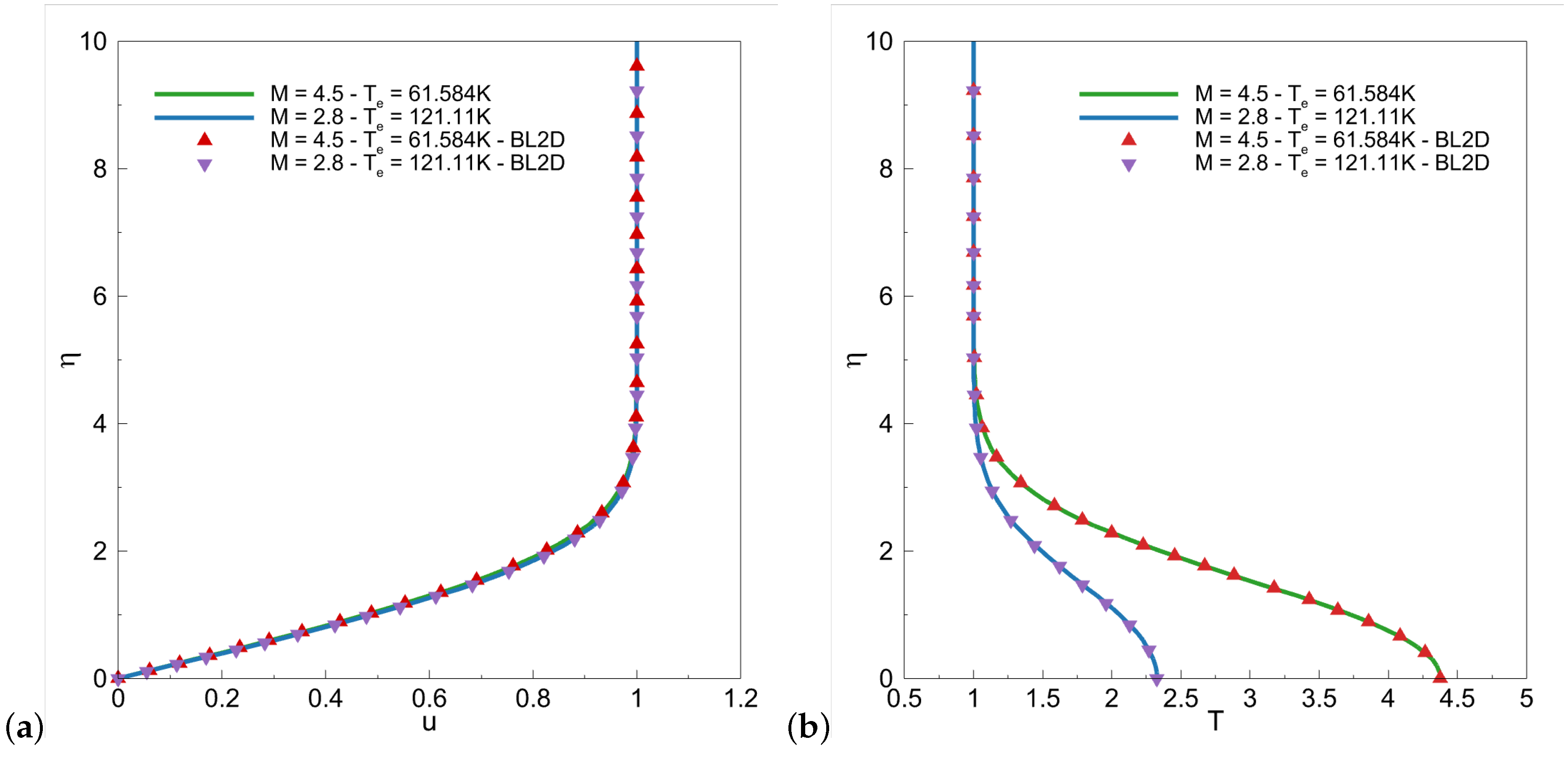
. The results of the code for
and
are illustrated in
Figure 3, where total temperatures are 311 K for both. The freestream temperature is calculated from isentropic relation and it is
K for
and
K for
. The results are compared with the Iyer’s [
20] BL2D boundary-layer solver, which is used in NASA’s well-known compressible boundary-layer stability solver LASTRAC [
21].
Listing 4.
Implementation of Newton’s Iteration Method in Julia environment. It requires three function calls to estimate the missing boundary condition value. Each estimation will lead to closer boundary condition guess.
Listing 4.
Implementation of Newton’s Iteration Method in Julia environment. It requires three function calls to estimate the missing boundary condition value. Each estimation will lead to closer boundary condition guess.


