Abstract
The Cook Strait in New Zealand is an ideal location for wind and tidal renewable sources of energy due to its strong winds and tidal currents. The integration of both technologies can help to avoid the detrimental effects of fossil fuels and to reduce the cost of electricity. Although tidal renewable sources have not been used for electricity generation in New Zealand, a recent investigation, using the MetOcean model, has identified Terawhiti in Cook Strait as a superior location for generating tidal power. This paper investigates three different configurations of wind, tidal, and wind plus tidal sources to evaluate tidal potential. Several simulations have been conducted to design a DC-linked microgrid for electricity generation in Cook Strait using HOMER Pro, RETScreen, and WRPLOT software. The results show that Terawhiti, in Cook Strait, is suitable for an offshore wind farm to supply electricity to the grid, considering the higher renewable fraction and the lower net present cost in comparison with those using only tidal turbines or using both wind and tidal turbines.
1. Introduction
The World Energy Outlook 2019 clarifies the effect of current decisions on energy systems in the future. If no policy actions are taken, then the current trend of energy demand is anticipated to increase by 1.30% per year until 2040, leading to an increase in emissions [1]. Today, with the increasing global energy demand and global climate change, two important solutions have been considered to tackle this issue: (i) reducing the cost of energy and (ii) finding new sources of energy that are environmentally friendly [2]. With the negative climate impact of fossil-fuel power generation and the requirement of global policy to shift towards a green mix of energy production, the investment in renewable energy is an opportunity in developing countries. However, a poor economy associated with limited income, funds availability, and regulations governing project funding and development are key factors that challenge investors in the energy sector [3].
In New Zealand, the Government set a target to reach 90% electricity production from renewable sources by 2025 [4,5] and 100% by 2035 [6]. Currently, there are 11,349 km of transmission lines that distribute electricity from remote areas, where generators are located, all over New Zealand. The Cook Strait cables connect the power line of the North Island to the South Island, as shown in Figure 1. These bi-directional cables carry 350 kW electricity [6].
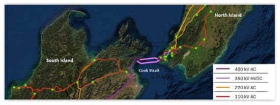
Figure 1.
Map of Cook Strait cables [7].
New Zealand consumes about 38,800 gigawatt-hours (GWh) of electricity per year. In 2017, renewable sources (hydro, geothermal, wind, and solar) supplied 59%, 17%, 5%, and 0.2% of the country’s electricity needs, respectively, and thermal sources (coal, diesel, and gas) supplied the other 18.8% [6].
Wind power systems are a cost-effective technology for harnessing renewable energy and have expanded annually at a dramatic rate of 25–35% globally over the last decade [8,9].
In more recent studies, the advantages of offshore wind generation against onshore wind generation have been highlighted through life cycle analysis (LCA), showing a 48% improvement in the sustainability of the project [10]. Offshore wind farms have increasingly attracted massive investment since 2015 [11]. However, the cost of electricity using offshore wind is still high [12]. Installing tidal turbines in New Zealand, as another good source of renewable energy, is usually considered to be not cost-effective because the turbines can be exposed to harsh currents that can reduce their life, and their foundation designs can be complicated in water deeper than 30 m [13].
Wind power systems, as a form of renewable energy source, are often integrated with other forms of power-generating systems to form a small power grid, known as a microgrid. The integration of both wind and tidal turbines using the same foundation reduces the cost of electricity [14] and enables a more predictable power generation from two different sources of energy.
The North and South Islands of New Zealand are separated by Cook Strait, connecting the Tasman Sea and the Pacific Ocean. It is 22 km wide at its narrowest point as shown in Figure 2 [15].
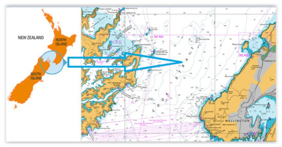
Figure 2.
Location of Cook Strait [16].
Much of the seabed is at water depths of less than 150 m, except through the Narrows, where depths reach greater than 300 m, and to the southeast in the Cook Strait canyon system [15].
The Cook Strait has been particularly explored due to the following unique features:
- strong convergent tidal flows in the context of a subtropical ocean convergence zone;
- the convergence of two crustal plates, underwater land sliding, and highly erosive currents; and
- wind funnelling and the associated high waves [17].
This paper investigates the best scenario in Cook Strait for a microgrid using wind and tidal energy as Cook Strait has the greatest potential for tidal energy in New Zealand. Three different scenarios of electricity generation are analyzed (i) using tidal turbines only, (ii) using wind turbines only, and (iii) using both wind and tidal turbines.
From a technical point of view, the contributions of the paper are as follows:
- Explore the use of tidal energy for on-grid design.
- Explore microgrid design to link tidal energy with other sources.
- Explore the use of optimization software as a method how to apply wind and tidal data into microgrid design.
- Define a method that could be used to optimize a microgrid of wind and tidal turbines anywhere to facilitate future feasibility studies.
HOMER Pro and WRPLOT view software are used for the integration of energy sources and analysing the resources’ potential. The HOMER Pro® microgrid software is used to optimize the off-grid and on-grid designs in both engineering and economic aspects for residential, commercial, and community purposes [18]. The WRPLOT view software is used to provide the available classes of turbine speeds for a given location [19].
2. Methods
HOMER (hybrid optimization model for multiple energy resources) [18] is used for the microgrid design of energy resources. Several simulations are carried out to design a DC-linked wind and tidal-based microgrid for electricity generation in the Terawhiti site in New Zealand. The resource conditions (wind speeds and tidal currents) can play an important role in selecting the microgrid components so that the microgrid can produce more electricity at a lower cost considering the technical constraints e.g., the 25-year project lifetime [20].
It is envisaged that the microgrid may also have the following:
- a biodiesel generator, as a backup to cover the base load from renewable sources in off-grid scenarios, and
- battery energy storage, for energy-storage applications.
There is also a need to investigate where the microgrid will link the offshore tidal and wind electricity outputs into the main grid. Several supply links may already exist, but if there is no supply link, a new link will have to be chosen.
The link should consist of:
- on-shore distribution lines, which can be overhead and underground lines with a percentage of distribution line losses; a
- transformer, to transfer electrical energy from one electrical circuit to another circuit; and a
- controller to manage or direct the load.
For the new hybrid wind and tidal system, other components will need to be purchased and installed. They are:
- support structures for tidal and wind turbines;
- tidal and wind turbines (including electrical generators);
- converters, to rectify the AC output of the generators to DC;
- marine cable, to feed power to a DC-AC converter at a site, then through an AC land cable to a system controller at a station; and a
- shore station, to feed the marine cable’s output into an AC network, where the cable emerges onto land.
To achieve islanded power generation, no grid is required, while, in a grid-connected system, there is a need to connect the output power of the generators to the grid [21]. Microgrids, either in grid-connected or islanded mode, could contribute to the future of clean energy by better controllability and adaptability [22].
The selection of the most economically viable project through the application of the incremental internal rate of return analysis can be affected by variations of any of the cash flow components, such as, for example, the capital cost, the operation, and maintenance cost, the fuel cost (as in the case of the diesel generator), the debt-to-equity ratio, the interest rate, etc. If a project is selected for investment, then it is to be funded by two resources. These are bank loans and promoters’ contributions. Bank loans reflect the debt component of the project cost and represent 75% of the capital cost of the project. On the other hand, promoters are to cover 25% of this cost [3].
There are two main electrical parameters for the optimization process; the total net present cost (NPC) and the levelized cost of energy (COE). The total value, which is calculated by HOMER for the installation, replacement, operation and maintenance, fuel, and the salvage of all components minus all the revenue during its lifetime, is the NPC or the life-cycle cost. The average generation cost of 1 kWh electricity is the COE [18].
Both of these parameters depend on the annualized cost of the system. The total NPC is calculated and can be expressed by (1) [23],
where is the total annualized cost, i is the actual interest rate, N is the number of years and is the capital recovery factor, which is calculated as,
The levelized cost of energy is given by,
where and are the amount of energy served by the microgrid and sold to the grid [20].
2.1. Site Selection
The Electricity Market Information website (EMI) [24] is part of the New Zealand Electricity Authority’s information website. Based on the facility location of the project, the microgrid considered in this study will be designed to provide the electricity demand to node CPK0331 (Central Park), in the south of the northern island of New Zealand, as shown in Figure 3.
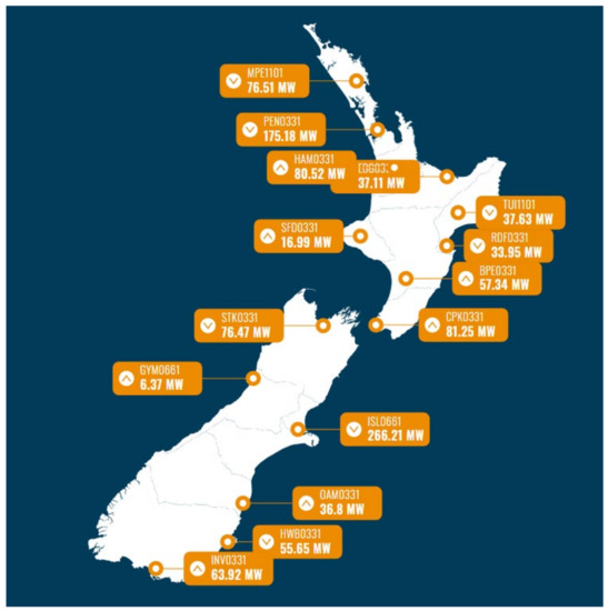
Figure 3.
Node load trends of New Zealand [25].
2.2. Identifying Demand
The EMI data has been used in the case study to estimate the monthly and hourly generation pattern as shown in Figure 4. Figure 4 shows that the peak (Figure 4a) and trough (Figure 4b) months are July and January, respectively [24].
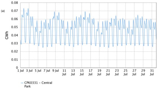
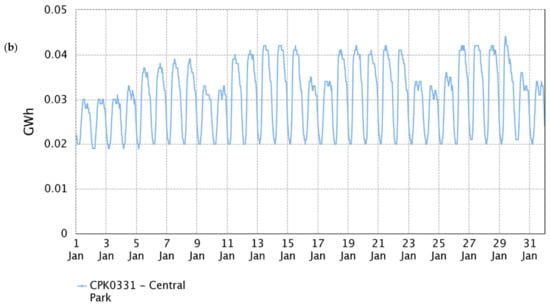
Figure 4.
(a) Maximum and (b) minimum load of CPK0331.
2.3. Obtaining Environmental Data
According to the MetOcean atmospheric model shown in Figure 5a, the tidal currents in four areas, (i) Cape Regina (in the north), (ii) Cook Strait (between two Islands), (iii) Foveaux Strait (in the north of Stewart Island), and (iv) south of Stewart Island are more than 1 m/second. The south of Stewart Island was ruled out as it is far from clients and markets and any installation there would increase the cost of the project significantly [26].
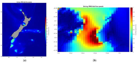
Figure 5.
Tidal current speeds (a) around New Zealand and (b) Terawhiti in cook strait.
So, for the microgrid design, two areas are suitable, (i) Cook Strait, in the south of the northern island, for the grid-connected design (Figure 5b), and (ii) the Foveaux Strait, in the south of the southern island, for the off-grid design on Stewart Island.
Tidal current modeling was conducted on an NZ-wide grid with a 0.06° resolution (5.6 × 6.6 km). The simulation nested high-resolution domains over Cook Strait (0.002°; 170 × 230 m). The tidal current around New Zealand is hindcasted by the Princeton Ocean Model (POM) in a vertically integrated two-dimensional mode with boundaries provided from the global TPX07.1 solution [26]. This model is the result of solving a set of partial differential equations of the spatial variability of tides using the Goring simplified continuity equation, the Navier-Stokes equations (by eliminating the vertical dimension-integrating velocities over depth), and a finite-element method [27].
The results showed that among these points, the Terawhiti point in Cook Strait has the strongest tidal currents for tidal power generation.
Global Wind Atlas [28] of New Zealand (Figure 6a) indicates that this point (Figure 6b) is also in an area with a high potential for wind energy.
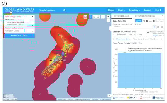
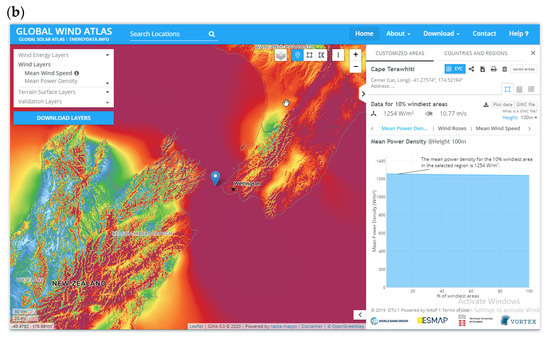
Figure 6.
Wind blow conditions in (a) New Zealand and (b) Terawhiti [28].

Table 1.
The environmental parameters of Terawhiti for microgrid design.
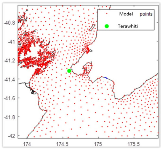
Figure 7.
Location of Terawhiti in Cook Strait.
2.4. Microgrid Components and Resources
To design a microgrid, the first step is to identify a site that is acceptable in terms of energy resources and power output and generation. This was done by contacting the National Institute of Water and Atmospheric Research (NIWA) and analyzing the wind and tidal conditions in those locations.
The next step is to import the resource data, such as wind and tidal current speeds. The wind speed values for the selected site can be automatically downloaded, from which the annual average wind speed can be calculated. However, the water speeds are not as easy to import, as HOMER needs hourly data from a 12-months period, which means a total of 8761 (total number of hours in a year) values of water speed need to be gathered and imported to HOMER to calculate the annual average water speed.
After that, various components need to be selected for the design including the data for the loads, wind and tidal turbines, convertor, controller, battery, and generator. The models and cost of all elements should be fed to HOMER. After completing the data entry, the simulation can proceed to analyze the cost–benefit comparison of the three technologies in these sites [20].
The main component for generating electricity from renewable energy resources (wind and tidal) is the turbine [29,30]. Wind and tidal turbines with similar capacities were selected from 19 Siemens SWT-3.6 MW-107 wind turbines and 38 AR2000 [2 MW] tidal turbines. The SWT-3.6–107 wind turbine was found to be an ideal offshore turbine. A strong structural design, self-regulating lubrication systems with great supplies, temperature control of the internal conditions, and a simple generator system without slip rings provide high reliability with long service periods. The unique net converter system for grid codes, from Siemens, has maximum flexibility in the output adjustments and faults. Also, in the design of the main components, best engineering practice needs to be used in terms of safety and dimension sizing [31]. The Siemens SWT 154, a6-MW turbine, marginally emerged as the favorable choice, using an options matrix from Plymouth University [32]. For the chosen tidal turbine, a comparable turbine of Siemens was chosen for the hybrid model.
A DC bus connects all the components, where, in this study, the wind and tidal turbines are the sources of energy. There is another setup in HOMER to choose the type of load profile that needs to be identified, such as residential, commercial, industrial, or community, where, in this study, the residential load was used. If energy storage is available, HOMER also requires the energy storage type. To ensure that the proposed microgrid can work autonomously, the Basf Nas 1250-kWh battery was chosen for storage set-up after many simulations [33].
The grid-connected system under consideration consists of wind and tidal turbines combined with a battery energy storage system (BESS) [34] to account for periods of prolonged lack of wind and tidal current, as shown in Figure 8.
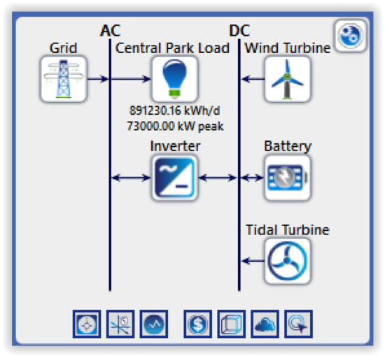
Figure 8.
Schematic layout of DC microgrid.
2.4.1. Wind Turbine
Figure 9 shows the power curve of the Siemens SWT-3.6–107 wind turbine. This turbine is the latest model from Siemens in the multi-MW class, having pitch technology with variable speed [35]. The capital, replacement, maintenance, and life of a turbine are taken as $6,000,000, $6,000,000, $120,000/year, and 20 years respectively. The power equation of the wind turbine is presented by Equation (4):
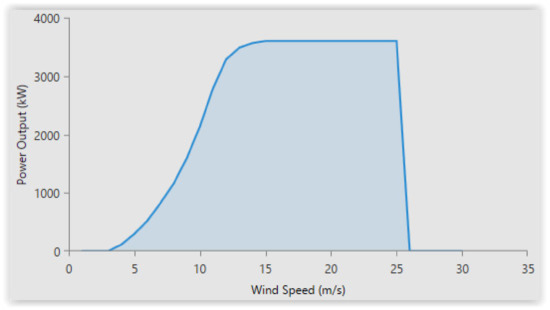
Figure 9.
The power curve of the Siemens SWT-3.6 MW-107 m offshore wind turbine [18].
The pertinent details for the Siemens SWT-3.6–107 wind turbine are set out in Table 2.
Table 2.
Wind turbine details [36,37].
The cut-in speed (the required wind speed for generating electricity) for the Siemens SWT-3.6 wind turbine is 4 m/s [38]. The WRPLOT viewing software [19] was used to find the wind frequency distribution in Terawhiti. Figure 10 shows that, for 78.2% of the year the wind speed, is greater than 4 m/s, hence it is suitable for electricity generation in Terawhiti.
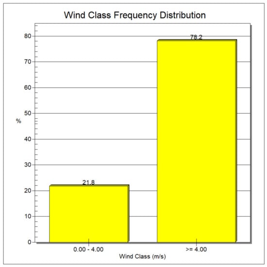
Figure 10.
Wind frequency distribution in Terawhiti.
2.4.2. Tidal Turbine
To understand the potential for tidal energy in New Zealand it is important to appreciate some unique features of its tidal patterns. The tidal pulls caused by lunar magnetism produce two high tides and two low tides over 24 h and travel around the New Zealand coast in about 12 h 25 min, which takes about 6 h 10 min for each incoming (flood) and outgoing (ebb) tide. The tide times vary from western New Zealand to eastern New Zealand (Waitemata harbor, Auckland and Manukau harbor, Auckland) in an anti-clockwise direction. Each harbor is adjacent to only a small piece of land with 4 h separating tidal patterns between the harbors (historical records show that Maori would take a canoe overland between Waitemata and Manukau harbors near Onehunga as a war party or for better fishing) [16]. Figure 11 is an example of a high tidal range site (Port Taranaki shown as Figure 11a) and a low tidal range site (Napier shown as Figure 11b), produced using TPX09 software [39].
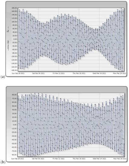
Figure 11.
(a) An example of a high tidal range site at Port Taranaki, and (b) a low tidal range site at Napier.
The diurnal inequality is more evident in Port Taranaki with a high tidal range. A strong complicated tidal current can be found through Cook Strait, between the North and South Islands [16]. The Terawhiti site which is investigated in this paper for microgrid design is in the Cook Strait area.
HOMER software provides different types of tidal turbines that are available in Hydrokinetic, a part of its library of components. Choosing two AR2000 tidal turbines, four cost parameter need to be fed to the software, (i) the capital (or installation and wiring and mounting expenses); (ii) the replacement cost; (iii) the maintenance cost; and (iv) the lifetime of the tidal turbines. For the purpose of this research, the following parameters were used: $3,000,000, $3,000,000, and $60,0000/year and 20 years, respectively. The power curves of the tidal turbine are given in Figure 12. The power equation of tidal turbine is presented by Equation (5):
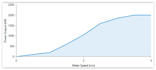
Figure 12.
The power curve of the AR2000 tidal turbine [18].
The pertinent details for the AR2000 tidal turbines are set out in Table 3.
Table 3.
Tidal turbine details.
Figure 13 shows that water speed, for 69.3% of the year, is greater than the cut-in speed required by the AR2000 tidal turbine.
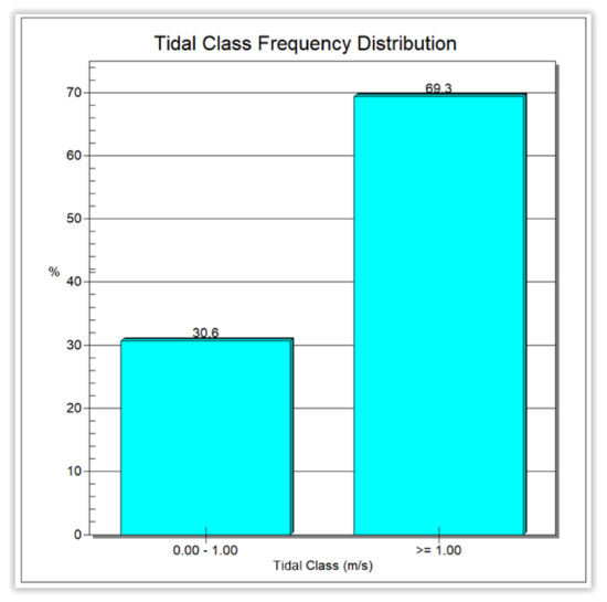
Figure 13.
Tidal frequency distribution in Terawhiti.
2.4.3. Battery Energy Storage
The integration of renewable sources requires proper storage backup [20]. The storage unit tabulated in Table 4 is a BASF NAS ® 192-volt battery with 1250 kWh of energy storage, due to its reliable performance and cost-effective operation. The capital, replacement, maintenance costs, and the life of the battery are given as $330,000, $330,000, $6,600/year, and 20 years, respectively [33].
Table 4.
Properties of BASF NAS ® battery [18].
2.4.4. Inverter
Inverters are required to connect the DC microgrid to the grid connection. The inverter used was a generic system inverter that is much cheaper than a bidirectional inverter. Selecting the HOMER optimizer parameter allows the HOMER grid to optimize the size of the inverter. The capital, replacement, maintenance costs, life, and efficiency of the converter were given as $154, $154, 15.4$/year, 15 years, and 90%, respectively [20].
2.4.5. Controller
The controller component specifies how the proposed system operates during the simulation. Among the dispatch strategies of the HOMER software, load following (LF) was selected to produce only enough power to meet demand. The capital, replacement, maintenance costs, and the life of the controller were given as $200, $200, $5/year, and 25 years, respectively [18].
2.4.6. Grid
For the simulation of the grid-connected system, ‘simple rates’ mode plus net metering was chosen. This type of design has two beneficial aspects; it considers emission factors and the timing when excess power is sold to the grid; HOMER calculates the power cost at the retail rate. So, net metering provides lower cost of production and greater income [18].
2.5. Optimizing the Design
Microgrid design optimization is possible because using HOMER Pro® has become a recognized global standard for off-grid and grid-connected systems [40]. The optimized scenario generates maximum electricity from renewable sources or has a higher renewable fraction.
2.6. Feasibility Analysis
As explained in Section 2, the economic analysis module of HOMER was used to estimate NPC and COE. Cost-effective analysis is an important part of the investigation to estimate the lowest possible NPC and COE [20].
3. Results and Discussions
Electricity Market Information data was used to estimate monthly and hourly generation. The peak hourly load was 73,000 kW. The EMI load is shown in Figure 14. The top graph (Figure 14a) shows that the average daily load fluctuated between 19,809 and 61,954 kW. The bottom graph (Figure 14b) shows that the average monthly load for different months of the year fluctuated between 20,419 and 39,354 kW in January and between 27,483 and 62,193 kW in July. The daily demand for the year averaged 891,230.16 kWh/d, with a load factor of 0.51, and the total demand is 325,299,008 kWh/year. [24].
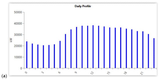
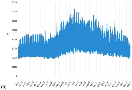
Figure 14.
(a) The daily and (b) monthly load of central park.
Resources are external parameters of the microgrid system that are required by HOMER. The selection of resources depends on the location and affects the power generation and financial viability of microgrid design and, hence, a careful choice is necessary for a successful analysis [23].
The resource types essential for this microgrid design are wind speed (downloaded by HOMER from the National Aeronautics and Space Administration (NASA), and water speed (provided by NIWA) for the year 2020.
Based on the resource frequency distribution, as shown in Figure 10 and Figure 13, the power that can be produced by the wind and tidal turbines at the Terawhiti site was chosen and is shown in Figure 15. The maximum output of the selected wind and tidal turbines are 3600 kW and 2000 kW, respectively, and Figure 15a for tidal turbine and Figure 15b for wind turbine indicate they can reach their rated output in Terawhiti at peak power.
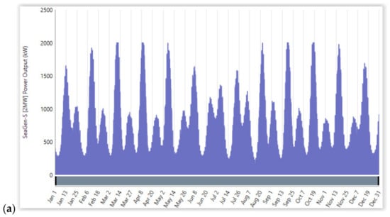
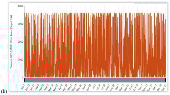
Figure 15.
Power output fluctuation for (a) tidal turbine and (b) wind turbine at the Terawhiti site.
Figure 16 compares the fluctuations in the power demand for three days, using the outputs obtained from the wind source (Figure 16a), tidal source (Figure 16b), and both wind and tidal sources (Figure 16c). Figure 16 show that the use of wind energy alone is better, when compared with the other designs.
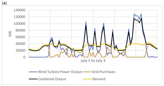
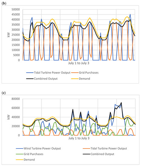
Figure 16.
Variation of required demand and power generation over three days at Terawhiti with (a) only wind turbine, (b) only tidal turbine, and (c) wind and tidal turbine.
The graphs in Figure 16 show that the higher the capacity of the wind or tidal power, the lower the grid energy purchased. Figure 17 shows the electrical load served from different cases vs consumption in the same period and shows that wind power can generate higher power and that purchasing from the grid is lower.
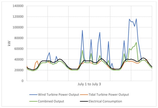
Figure 17.
Electrical consumption over three days at Terawhiti versus electrical load served by the wind turbine, tidal turbine, and wind and tidal turbine combination.
Section 3.1 and Section 3.2 evaluate different designs, using the HOMER software to optimize the turbine and generator operations, to meet the demand fluctuations throughout the year. Section 3.3 and Section 3.4 discuss the results, in terms of power generation and cost-effectiveness, respectively. The number of turbines used was 36 wind turbines (36 W), 113 tidal turbines (113 T), and a combination of 19 wind and 38 tidal turbines (19 W + 38 T).
3.1. Power Generation Results
Table 5 shows the mean output, the hours of operation, and the total production for each scenario. The number of turbines for each scenario is proportional to the amount of power consumption. The total power demand from Central Park is 325,299,008 kWh/year.
Table 5.
The annual mean output, hours of operation, and power production for the proposed scenarios at the Terawhiti site.
Figure 18a–c shows the monthly average power output (kW) and the share of resources for different scenarios. The renewable fraction of wind-only scenario (36 W) is 66.3%, which is higher than the tidal-only scenario (63.9%) and the combined wind and tidal sources (65.4%).
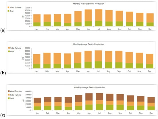
Figure 18.
Monthly average output power for (a) 36 W, (b)113 T, (c) 19 W + 38 T.
HOMER results indicates that for the 36 W scenario, 122,551 kWh/year energy is lost due to battery loss and battery storage depletion, which is lower than 113 T and 19 W + 38 T scenarios, which lost 396,486 and 273,186 respectively. Also, the mean output of the inverter in 36 W was 32,738 kW, which was higher than 113 T and 19 W+38 T scenarios, which output 32,187 and 27,983 respectively. The annual output of the inverter is shown in Figure 19.
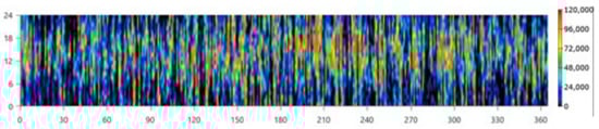
Figure 19.
Annual inverter output for 36 W.
The efficiency of the inverter, in all calculations, was 90%. The sensitivity analysis to the inverter efficiency was performed at increments of 5%, as shown in Table 6. According to the sensitivity analysis of the inverter efficiency, the wind project was still the most technically viable.
Table 6.
Sensitivity analysis of inverter efficiency on decision-making.
3.2. Financial Analysis Results
Table 7 is a summary of financial analysis for different scenarios at the Terawhiti site.
Table 7.
Financial analysis results for different scenarios.
The 36 W scenario seems more economical to install and operate. Table 8, Table 9, Table 10 depicts the optimization results for each scenario. The renewable fractions are 66.3%, 63.9%, and 65.4% respectively. A renewable fraction (RF) of 66.3% means that 66.3% of electricity is supplied from wind turbines and the rest from the grid. Hybrid systems with a renewable fraction of more than 66% can produce high revenue. [41]. The 36 W wind turbine meets this criterion. It has lower capital and operating costs and a lower NPC than the 113 T or 19 W + 38 T turbines, and most importantly, it has a lower COE.
Table 8.
Optimization results for 36 W.
Table 9.
Optimization results for 113 T.
Table 10.
Optimization results for 19 W + 38 T.
Table 11 and Figure 20 show the scenario with the lowest costs at the Terawhiti site, the net present cost of each component in the system, and the system cost as a whole. The replacement and salvage costs are small. The main costs are capital and operating costs.
Table 11.
Components of NPC for the scenario with the lowest NPC (36 W).
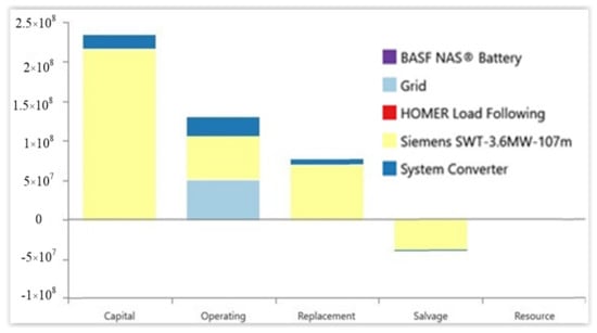
Figure 20.
Cost summary for the 36 W scenario.
HOMER provides an overview of the winning system—the system with the lowest net present cost in comparison to the base system. The base-case system is the system with the lowest initial capital cost. There could be scenarios wherein the base-case system is also the winning system. According to Table 7, the NPC of the winning 36 W system is 400 M$, which is lower than the 586 and 456 M$ for 113 T and 19 W+38 T, respectively. This value is also lower than the NPC of the base system (421 M$) for 36 W. Figure 21 shows how the winning system of 36 W can save money over the project lifetime.
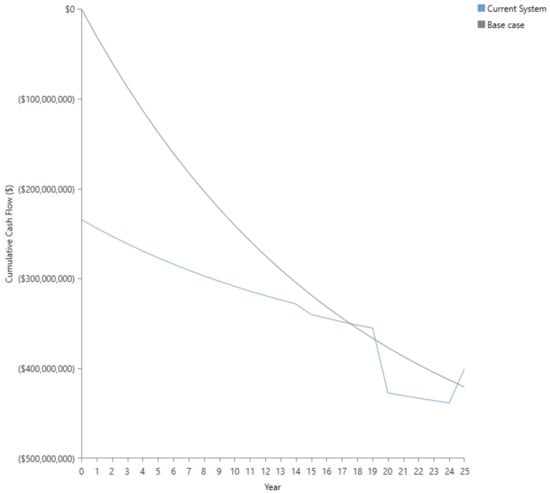
Figure 21.
Cumulative cash flow of 36 W.
A sensitivity analysis was conducted to examine the impact of capital cost, operation, and maintenance cost on the selection decision, considering the comparison of the different scenarios discussed above. The project capital and the operation, and maintenance cost are allowed to vary between 10% and −10% at increments of 5%, using RETScreen [42]. Table 12 serves as a guide to interested investors on the best option for investment among the W, T, and W+T projects when considering such variations. Table 12 shows that the corresponding capital variation in the projected internal rate of return is in the range of [15.7%, 20.3%] for W, [9.5%, 13.3%] for T, and [9.4%, 13.2%] for W+T and the corresponding O and M variation in the projected internal rate of return is in the range of [17.5%, 18.1%] for W, [11.1%, 11.5%] for T, and [10.9%, 11.3%] for W+T. According to the incremental internal rate of return analysis, the wind project was the most economically viable project when considering the variation in the capital and O and M costs between −10% and 10% of the total cost of the project, compared with the others. The minimum acceptable rate of return (MARR) was determined to be 14%. Table 12 shows that the T and W+T projects are rejected, as their calculated IRR values are less than the MARR.
Table 12.
Sensitivity analysis of capital and O and M costs on decision-making.
Economic assessment using the incremental rate of return method [43] and the application of sensitivity analysis on the capital cost and operation and maintenance cost to select the best economic project among wind, tidal, and combination of wind and tidal projects revealed that 36 W is a more attractive and feasible option compared to other distributed generation projects.
3.3. Discussion of Power Generation Results
Table 13 shows the mean output power for all scenarios. Central Park’s mean power demand is 37,134.6 kW. All scenarios can meet the mean demand, but none of the total outputs can meet the peak demand (73,000 kW).
Table 13.
Mean output for different scenarios.
Table 14 shows the percentage of the electricity produced by the wind and tidal turbines. Central Park’s total power demand is 325,299,008 kWh/year. The 36 W wind turbine produces the highest renewable energy fraction and could contribute 68.6% of power demand.
Table 14.
Share of wind and tidal turbines in producing electricity and meeting demand.
Comparing different designs shows that the 36 W wind turbine is the best design for meeting the electricity demand of Central Park by wind.
Although the MetOcean model indicates that Terawhiti is in an area with the New Zealand’s highest tidal energy, the renewable fraction of the 36 W wind turbine is higher than in other scenarios. Based on the calculations, the ratio of renewable production to total consumption is considered to be 73% for all scenarios. The wind energy-only option can maximize its contribution and minimize the grid purchases in comparison with the other cases.
3.4. Discussion of Financial Analysis Results
In this section, the scenarios are compared, based on the financial analysis results from Section 3.2, which are summarized in Table 15.
Table 15.
Financial analysis summary.
Capital equipment/ Replacement: The cost is least for the 36 W wind turbine scenario.
Construction: The cost of project installations is not shown, because HOMER Pro’s financial analysis module does not include it (it only compares equipment, operating, and resource costs).
Removal/reinstatement: The cost to remove or re-instate project installations (at end of design life) is not shown, for the same reason as above.
Operation: The cost is the least for the 36 W wind turbine scenario, which generates more power from fewer turbines. The operating cost for the 113 T tidal turbine scenario is greater because this scenario has numerous turbines. The operating cost is most expensive for the scenarios that generate less power from renewable sources.
The total net present cost (NPC): The NPC is the least for the 36 W wind turbine scenario because this scenario has low equipment and operating costs and generates more power (68.6%) from renewable sources.
The total cost of energy: the COE is the least for the 36 W wind turbine scenario and almost the same for the 113 T and 19 W+38 T scenarios when their NPCs are levelized (per kWh over the life of the project).
The 36 W wind turbine scenario is optimal for power generation because it produces the highest renewable fraction (66.3%), while the RF for the 19 W + 38 T and 113 T scenarios are 65.4% and 63.9%, respectively. Its total NPC seems affordable at 400 million dollars. Its levelized cost, at 7 c/kWh, appears better than the investment in tidal energy, based on the tidal models.
A problem with HOMER Pro’s financial analysis is that it only evaluates equipment, operating, and resource costs when calculating NPC and COE. A realistic comparison of NPC and COE should include the construction and installation costs, particularly for the offshore platforms, marine cables, and a DC-AC shore converter station.
4. Conclusions
This paper has investigated a DC-linked wind-tidal battery-based microgrid for electricity generation in node CPK0331 (Central Park) in the south of the northern islands of New Zealand. The system considered the good potential of wind and tidal sources in this area to design an environmental-friendly microgrid connecting to the national grid with cheaper electricity generation.
Many simulations were conducted to design the DC-linked microgrid for integration with the electricity grid to supply the residential load in Terawhiti. Based on the selection of components, and by including the resource data of the wind speed and tidal currents, the microgrid design provides the capacity and cost for different options.
HOMER Pro was used to compare different scenarios and propose an optimized microgrid system and the required components thereof to generate maximum power from renewable sources with the lowest cost of generation.
The power generation and financial analysis results for the various scenarios, as presented and discussed in Section 3, enable several conclusions:
- ▪
- There are enough tidal currents to generate electricity during 69.3% of the year at an offshore site close to CPK0331 (referred to as the Central Park).
- ▪
- There is also enough wind speed to generate electricity during 78.2% of the year at the Foveaux site.
- ▪
- The DC power from the offshore Terawhiti site can be integrated into the national grid at CPK0331 by using the microgrid design described in Section 2.
- ▪
- The proposed solution is to mount the wind and tidal turbines on the same offshore platform, design a DC-linked wind-tidal-battery-based microgrid to feed the power through a DC marine cable to a DC-AC converter at the CPK0331 onshore, then transmit the power through an AC land cable to a system controller at the Central Park station.
- ▪
- The offshore renewable sources enable several scenarios to provide the demand of Central Park with HOMER Pro, which looks promising. The optimal scenario generating maximizing electricity is thirty-six wind turbines (36 W).
- ▪
- The renewable output of 68.6% from the 36 W scenario (look at Table 14) is worth implementing, when compared with the other scenarios.
- ▪
- Once built and installed on-site, the design can be operated at an affordable levelized cost of 7 c/kWh (look at Table 6) over the project life, which is lower than adding the tidal source.
Author Contributions
Conceptualization, N.M.N., M.R.I., K.M. and D.S.; methodology, N.M.N., M.R.I., K.M. and D.S.; software, N.M.N.; formal analysis, N.M.N.; resources N.M.N., M.R.I. and D.S.; writing—original draft preparation, N.M.N., M.R.I. and D.S.; writing—review and editing, N.M.N., M.R.I. and D.S.; supervision, N.M.N., M.R.I., K.M. and D.S.; project administration, N.M.N.; All authors have read and agreed to the published version of the manuscript.
Funding
This research received no external funding.
Informed Consent Statement
Not applicable.
Data Availability Statement
Data available on request from the authors.
Acknowledgments
The authors wish to acknowledge the technical support of Julie Jakoboski from MetOcean and Craig Stewart from NIWA.
Conflicts of Interest
The authors declare no conflict of interest.
References
- World Energy Outlook 2019-Flagship Report-November 2019. Available online: https://www.iea.org/reports/world-energy-outlook-2019 (accessed on 7 November 2021).
- Algarvio, H.; Lopes, F.; Santana, J. Strategic Operation of Hydroelectric Power Plants in Energy Markets: A Model and a Study on the Hydro-Wind Balance. Fluids 2020, 5, 209. [Google Scholar] [CrossRef]
- Saad Al-Sumaiti, A.; Kavousi-Fard, A.; Salama, M.; Pourbehzadi, M.; Reddy, S.; Rasheed, M.B. Economic Assessment of Distributed Generation Technologies: A Feasibility Study and Comparison with the Literature. Energies 2020, 13, 2764. [Google Scholar] [CrossRef]
- Parker, H.D. New Zealand Energy Strategy to 2050: Powering Our Future; New Zealand Government: Wellington, New Zealand, 2007.
- Efficiency, E.; Authority, C. New Zealand Energy Efficiency and Conservation Strategy; EECA: New Zealand, 2007. Available online: https://www.beehive.govt.nz/sites/default/files/Energy_Efficiency_and_Conservation_Authority_BIM_0.pdf (accessed on 1 October 2021).
- Electricity in New Zealand; Electricity Authority: New Zealand, 2018. Available online: https://www.ea.govt.nz/about-us/media-and-publications/electricity-new-zealand/ (accessed on 1 October 2021).
- Transpower Geospatial Map. Available online: https://data-transpower.opendata.arcgis.com/ (accessed on 21 September 2021).
- Roy, L.; Kincaid, K.; Mahmud, R.; MacPhee, D.W. Double-Multiple Streamtube Analysis of a Flexible Vertical Axis Wind Turbine. Fluids 2021, 6, 118. [Google Scholar] [CrossRef]
- Lu, M.-S.; Chang, C.-L.; Lee, W.-J.; Wang, L. Combining the wind power generation system with energy storage equipment. IEEE Trans. Ind. Appl. 2009, 45, 2109–2115. [Google Scholar]
- Noori, M.; Kucukvar, M.; Tatari, O. Economic input–output based sustainability analysis of onshore and offshore wind energy systems. Int. J. Green Energy 2015, 12, 939–948. [Google Scholar] [CrossRef] [Green Version]
- Lande-Sudall, D.; Stallard, T.; Stansby, P. Energy yield for co-located offshore wind and tidal stream turbines. In Proceedings of the 2nd International Conference on Renewable Energies, London, UK, 26–28 July 2016; pp. 675–681. [Google Scholar]
- Heptonstall, P.; Gross, R.; Greenacre, P.; Cockerill, T. The cost of offshore wind: Understanding the past and projecting the future. Energy Policy 2012, 41, 815–821. [Google Scholar] [CrossRef]
- Lande-Sudall, D.; Stallard, T.; Stansby, P. Co-located offshore wind and tidal stream turbines: Assessment of energy yield and loading. Renew. Energy 2018, 118, 627–643. [Google Scholar] [CrossRef]
- Gruszczynski, A.; Hambrey, D.; Jiménez, E.; Sagan, I.; Sheaikh, S.; Viana, L. Hybrid Offshore Wind and Tidal. Available online: http://www.esru.strath.ac.uk/EandE/Web_sites/16–17/WindAndTidal/index.html (accessed on 8 September 2017).
- Mountjoy, J.J.; Barnes, P.M.; Pettinga, J.R. Morphostructure and evolution of submarine canyons across an active margin: Cook Strait sector of the Hikurangi Margin, New Zealand. Mar. Geol. 2009, 260, 45–68. [Google Scholar] [CrossRef]
- Linz Information about Tides around New Zealand. Available online: https://www.linz.govt.nz/sea/tides/introduction-tides/tides-around-new-zealand (accessed on 4 February 2021).
- Walters, R.A.; Gillibrand, P.A.; Bell, R.G.; Lane, E.M. A study of tides and currents in Cook Strait, New Zealand. Ocean Dyn. 2010, 60, 1559–1580. [Google Scholar] [CrossRef]
- Homer Pro. Available online: https://www.homerenergy.com/ (accessed on 2 March 2020).
- WRPLOT View™—Freeware. Available online: https://www.weblakes.com/products/wrplot/index.html (accessed on 8 July 2020).
- Phurailatpam, C.; Rajpurohit, B.; Wang, L. Optimization of DC microgrid for rural applications in India. In Proceedings of the 2016 IEEE Region 10 Conference (TENCON), Singapore, 22–25 November 2016; pp. 3610–3613. [Google Scholar]
- Hatziargyriou, N. Microgrids: Architectures and Control; John Wiley & Sons: Hoboken, NJ, USA, 2014. [Google Scholar]
- Roberts, D.; Chang, A. Meet the Microgrid, the Technology Poised to Transform Electricity. Vox. May 2018, 24, 2018. [Google Scholar]
- Lambert, T. Micropower System Modeling with Homer; Wiley-IEEE Press: Toronto, ON, Canada, 2006. [Google Scholar]
- Electricity Authority Information of New Zealand. Available online: https://www.emi.ea.govt.nz/ (accessed on 25 July 2021).
- Node Load Trends of New Zealand. Available online: https://www.ems.co.nz/services/em6/ (accessed on 12 January 2020).
- Huckerby, J.; Johnson, D. New Zealand’s wave and tidal energy resources and their timetable for development. In Proceedings of the International Conference on Ocean Energy (ICOE), Brest, France, 15–17 October 2008; pp. 15–17. [Google Scholar]
- Goring, D. Computer models define tide variability. Ind. Phys. 2001, 7, 14–17. [Google Scholar]
- Global Wind Atlas. Available online: https://globalwindatlas.info/ (accessed on 20 December 2020).
- Rakhshani, E.; Mehrjerdi, H.; Iqbal, A. Hybrid wind-diesel-battery system planning considering multiple different wind turbine technologies installation. J. Clean. Prod. 2020, 247, 119654. [Google Scholar] [CrossRef]
- Benato, A.; De Vanna, F.; Gallo, E.; Stoppato, A.; Cavazzini, G. TES-PD: A Fast and Reliable Numerical Model to Predict the Performance of Thermal Reservoir for Electricity Energy Storage Units. Fluids 2021, 6, 256. [Google Scholar] [CrossRef]
- Siemens Wind Turbine SWT-3.6–107. Available online: https://www.renugen.co.uk/content/large_wind_turbine_brochures/large_wind_turbine_brochures/siemens_swt-3.6–107.pdf (accessed on 14 June 2021).
- Offshore Renewable Energy for Guernsey. Available online: http://www.guernseyrenewableenergy.com/documents/managed/Offshore%20Renewable%20Energy%20for%20Guernsey.pdf (accessed on 14 June 2021).
- Phurailatpam, C.; Rajpurohit, B.S.; Wang, L. Planning and optimization of autonomous DC microgrids for rural and urban applications in India. Renew. Sustain. Energy Rev. 2018, 82, 194–204. [Google Scholar] [CrossRef]
- El-Bidairi, K.S.; Nguyen, H.D.; Mahmoud, T.S.; Jayasinghe, S.; Guerrero, J.M. Optimal sizing of Battery Energy Storage Systems for dynamic frequency control in an islanded microgrid: A case study of Flinders Island, Australia. Energy 2020, 195, 117059. [Google Scholar] [CrossRef]
- Recordon, E. Siemens Energías Renovables; CIGRE: Chile, 2009; Available online: https://www.cigre.cl/wp-content/uploads/2017/03/Siemens-Recordon.pdf (accessed on 1 October 2021).
- Karimirad, M. Offshore Energy Structures: For Wind Power, Wave Energy and Hybrid Marine Platforms; Springer: Oslo, Norway, 2014. [Google Scholar]
- Bhattacharya, S. Design of Foundations for Offshore Wind Turbines; Wiley Online Library: Hoboken, NJ, USA, 2019. [Google Scholar]
- Mitchell, S.; Ogbonna, I.; Volkov, K. Aerodynamic characteristics of a single airfoil for vertical axis wind turbine blades and performance prediction of wind turbines. Fluids 2021, 6, 257. [Google Scholar] [CrossRef]
- Tidal Prediction Using TPX09. Available online: http://oceanomatics.com/ (accessed on 8 December 2020).
- Deshmukh, M.; Singh, A.B. Modeling of Energy Performance of Stand-Alone SPV System Using HOMER Pro. Energy Procedia 2019, 156, 90–94. [Google Scholar] [CrossRef]
- Hiendro, A.; Ismail, Y.; Wigyarianto, F.T.P.; Khwee, K.H.; Junaidi, J. Optimum Renewable Fraction for Grid-connected Photovoltaic in Office Building Energy Systems in Indonesia. Int. J. Power Electron. Drive Syst. 2018, 9, 1866. [Google Scholar] [CrossRef]
- RETScreen. Available online: https://www.nrcan.gc.ca/maps-tools-publications/tools/data-analysis-software-modelling/retscreen/7465 (accessed on 4 June 2020).
- Newnan, D.G.; Eschenbach, T.; Lavelle, J.P. Engineering Economic Analysis; Oxford University Press: Oxford, UK, 2004; Volume 2. [Google Scholar]
Publisher’s Note: MDPI stays neutral with regard to jurisdictional claims in published maps and institutional affiliations. |
© 2021 by the authors. Licensee MDPI, Basel, Switzerland. This article is an open access article distributed under the terms and conditions of the Creative Commons Attribution (CC BY) license (https://creativecommons.org/licenses/by/4.0/).