Abstract
In the computational mechanics of multiphase dispersed flows, there is an issue of computing the interaction between phases in a mixture of a carrier fluid and dispersed inclusions. The problem is that an accurate dynamics simulation of a mixture of gas and finely dispersed solids with intense interphase interaction requires much more computational power compared to pure gas or a mixture with moderate interaction between phases. To tackle this problem, effective numerical methods are being searched for to ensure adequate computational cost, accuracy, and stability of the results at an arbitrary intensity of momentum and energy exchange between phases. Thus, to assess the approximation, dispersive, dissipative, and asymptotic properties of numerical methods, benchmark solutions of relevant test problems are required. Such solutions are known for one-dimensional problems with linear plane waves. We introduce a novel analytical solution for the nonlinear problem of spherically symmetric expansion of a gas and dust ball into a vacuum. Therein, the dynamics of carrier and dispersed phases are modeled using equations for a compressible inviscid gas. Solid particles do not have intrinsic pressure and are assumed to be monodisperse. The carrier and dispersed phases exchange momentum. In the derived solution, the velocities of gas and dust clouds depend linearly on the radii. The results were reproduced at high, moderate, and low momentum exchange between phases using the SPH-IDIC (Smoothed Particle Hydrodynamics with Implicit Drag in Cell) method implemented based on the open-source OpenFPM library. We reported an example of using the solution as a benchmark for CFD (computational fluid dynamics) models verification and for the evaluation of numerical methods. Our benchmark solution generator developed in the free Scilab environment is publicly available.
1. Introduction
The coupled dynamics of gas and solid particles underlies a large variety of natural phenomena and technology-driven processes. In this paper, we consider the dynamics of a mixture where the boundary between gas and solid inclusions is irrelevant; that is, solid particles are dispersed in a carrier gas. Such systems are called dispersed media. A number of mathematical models have been designed to investigate coupled gas and particles dynamics at different scales (e.g., [1,2,3,4]). In particular, macro and meso level models are used for dispersed media simulation. The description of a medium at a macro level involves the use of volume-averaged characteristics (density, velocity, internal energy) for both the carrier and dispersed phases. In this case, fluid dynamics (of the entire mixture or separately of the carrier and dispersed phases) are modeled using gas dynamics equations. A meso level description means applying kinetic equations to simulate gas and/or dispersed particles. In kinetic equations, as opposed to fluid dynamics equations, the velocity at any given point of space is not unique but has a spectrum of values.
Let us assume that both carrier and dispersed phases in the mixture are inviscid. If the mass or volume fraction of the dispersed phase is considerable (the mixture is dense), then the mixture dynamics are essentially impacted by the mutual exchange of energy and momentum between phases. Such exchange is modeled by introducing corresponding relaxation terms in the right-hand sides of the momentum and energy equations. Examples of such dense mixtures of solids and gas include fluidized bed chemical reactors (e.g., [1]), astrophysical protoplanetary disks, in which planets are formed (e.g., [5]), and other objects.
In the computational mechanics of dense inviscid dispersed media, computing the interaction between phases constitutes a problem. It is known that simulating the dynamics of a mixture of a carrier gas and finely dispersed solids with fast momentum and energy exchange between phases requires much more computational power compared to pure gas or mixture with moderate interaction between phases. To tackle this problem, effective numerical methods are searched for to ensure adequate computational cost, accuracy, and stability of the results at arbitrary interphase exchange rates. Thus, benchmark solutions of dynamics problems for mixtures with arbitrary interphase interaction are highly sought to evaluate the approximation, dispersive, dissipative, and asymptotic properties of numerical methods. A corresponding system of benchmark tests has been developing in recent decades. It includes problems of particle drift in either a stationary or rotating gaseous medium, classical inviscid pure gas dynamics generalized to a gas and dust medium, and solutions describing phenomena specific to a two-phase fluid. In what follows we review several solutions for gas and dust dynamics that are used to verify the computational fluid dynamics codes (primarily by the astrophysical community).
The authors of [6] introduced a solution for a single particle drifting under the gravitational force of a massive central body in an equilibrium gas cloud with Keplerian differential rotation. The particle does not affect the gas dynamics. This solution was further extended by [7] into the case of a gas cloud with non-zero radial velocity. The authors of [8,9] generalized this solution to a polydisperse dust cloud that is not a passive admixture but exchanges momentum with the carrier gas.
Analytical solutions of propagation of small amplitude acoustic waves in a gas and dust mixture are commonly used to assess the dissipative and dispersive properties of numerical methods. The authors of [10] derived the wave group velocity in a monodisperse dusty gas under the approximation of instant momentum exchange (relaxation equilibrium). The solution of a propagating monochromatic wave in a mixture of gas and monodisperse dust at an arbitrary relaxation time was introduced to the practice of astrophysical simulator verification in [11]. The authors of [8] extended this solution into the case of a mixture of gas and polydisperse dust. The authors of [12,13] generalized the monodisperse and polydisperse mixture solutions, respectively, to including particles buoyancy.
The Sod problem (Riemann problem) of the decay of a strong discontinuity in density, pressure, and internal energy represents a classical test for one-dimensional equations for inviscid gas dynamics. A numerical solution to this problem requires introducing an artificial viscosity or using Riemann solvers. This problem has a generalization to the case of a gas and dust mixture with negligible dust volume. Its non-stationary solution for a mixture under relaxation equilibrium was used as a code verification benchmark, for example, in [14,15] (for monodisperse mixtures) and [16] (for polydisperse mixtures). Additionally, the authors of [17] introduced a stationary solution of the Riemann problem for a monodisperse mixture as a benchmark for numerical code verification.
In the case of two dimensions, the numerical solution for inviscid dusty gas dynamics was tested by simulating the streaming instability that results from the differential rotation of a carrier gas and the momentum exchange between gas and dispersed particles [18]. The problem of streaming instability development in the shearing box approximation was used as a CFD verification test for monodisperse [19] and polydisperse [8] mixtures.
Spherically symmetric problems of inviscid gas dynamics, such as Noh, Guderley, and Sedov’s problems, are classical verification tests for three-dimensional CFD implementations. To our best knowledge, they have not been generalized to a gas and dust medium to date, even for the limiting case of relaxation equilibrium when the gas and dispersed phase velocities almost coincide. This paper handles the spherically symmetric problem of a mixture of inviscid gas and dispersed particles expanding into a vacuum, for which we managed to derive a new benchmark solution with arbitrary values of velocity relaxation time. This problem helps to verify a CFD code in three dimensions even at a coarse spatial resolution and to examine the asymptotic, dispersive, and dissipative properties of numerical methods for two-phase dispersed flows.
In Section 2, a brief overview of previous results of similar problems involving pure gases is provided (Section 2.1), the benchmark solution derivation for a mixture of gas and dust is described (Section 2.2), a code generating the benchmark solution is numerically introduced (Section 2.3), and the comparison of the newly derived solution to previous analytical results is presented (Section 2.4). Section 3 describes the SPH-IDIC method for gas and dust dynamics and its implementation based on the open-source OpenFPM library. In Section 4, we demonstrate that the derived solution can be reproduced at extreme and moderate relaxation time values. The conclusions are outlined in Section 5.
2. Benchmark Solution for Gas and Dust Ball Expansion into Vacuum
2.1. Regular Expansion of a Gas Cloud into Vacuum—Brief Outline of Previous Results
The expansion of inviscid gas into a vacuum under its own pressure is a classical fluid mechanics problem. Solutions to this problem are examined with analytical and numerical methods. In particular, a family of solutions to this problem is well explored analytically that describes the velocity of expanding gas as a linear function of the distance from the symmetry center at rest. Such solutions are called regular, or solutions with a uniform velocity gradient. Solutions for the spherically symmetric gas expansion problem with a uniform velocity gradient have been known from the middle of the twentieth century [20,21,22,23]. Further on, the regular solution of the gas ball expansion problem was generalized to the cases of a three-axial ellipsoid [24] and a rotating two-axial ellipsoid [25]. The general approach to these solutions includes: (1) using spherical coordinates; (2) representing all gas macro parameters as products of functions exclusively depending either on time or on the position of a point in the expanding cloud; (3) integrating the initial partial differential equations by variable separation; (4) proceeding either to an ordinary second-order differential equation for the ball radius or to a system of ordinary differential equations for the radii of the ellipsoid principal axes. In the following years, solutions to the problem of a gas cloud expanding into a vacuum were systematically studied and applied in various subject areas. For example, in [26,27] solutions with a uniform velocity gradient were found for gas dynamics in a stationary self-consistent gravitational field for astrophysics (see reviews in [28,29]). A recent contribution [30] provided a general form of known regular solutions for equations of inviscid gas without additional external forces. A comprehensive overview of the literature on the subject, the consecutive derivation, and classification of the known families of regular solutions for a two-axial ellipsoid were provided.
In this paper, we introduce a spherically symmetric problem of expansion into a vacuum of a mixture of inviscid gas and dispersed particles. Using the variable separation method, we managed to construct a novel benchmark solution for arbitrary velocity relaxation time values. This setting generalizes the known solution of the dynamics of a pure gas ball expanding into a vacuum with a uniform velocity gradient and homogeneous density (see [23,30] p. III.B.1) to the case of a gas and dust mixture.
2.2. Problem Description and Derivation of the Analytical Solution
The diagram of gas and dust medium expansion is given in Figure 1.
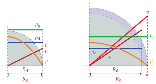
Figure 1.
The sketch of spherically symmetric gas and dust cloud free expansion. The left and right panels show the distribution of macroscopic parameters for a gas and dust mixture at the initial time moment and at a given time, respectively.
A gas and dust medium with mass , where is the mass of gas and is the mass of dust particles, is modeled as two concentric spheres with radii and respectively, centered at the origin. We assume that the gas ball has zero values of viscosity and heat conductance. For the cloud of dust particles, the averaged values of density and velocity are defined for any point inside the ball. Next, we assume that the gas and particles exchange momentum, however, there is no transfer of mass or energy between the phases. Let the distribution of gas pressure and velocities in the gas and particles be spherically symmetric at the initial time moment. Assume that the system expands freely into a vacuum. This means that the distribution of macro parameters remains spherically symmetric during the expansion. Hence, the dynamics of the system can be described by one-dimensional gas dynamic equations in the spherical coordinates:
where t is the time, r is the distance to the center of the ball, is the gas density, is the volume density of dust particles (loose powder density), is the internal energy of gas, is the pressure, are the gas and dust radial velocities, respectively, and is the time of relaxation of the particles velocity to the gas velocity. In the most general case, depends on the particle parameters (shape, size, and material), as well as on the parameters of the gas. To derive an analytic solution, we assume that the parameter is unchanged during the motion of the gas and dust cloud. It should be noted that the set of Equation (1) is consistent only at , where , are the radii of gas and dust balls, respectively. To close the system (1), we add the ideal gas equation of state
where is the adiabatic exponent, which is a free parameter of the problem. We assume now that the pressure gradient and the drag force ensure the motion of the whole assembly, such that for any time moment the gas density in the gas ball and the dust density in the dust ball are independent on the space coordinates, while the ball radii are changing over time:
Then the continuity equation requires a linear dependence of gas and dust velocities on r. Indeed, from (3) the first equation in (1) can be cast as
where the first term is a function of time and does not depend on the space point. From here it follows that the second term is also a function of time and independent of the coordinates, that is
After variables separation, we get the expression for the gas velocity
To ensure that the gas velocity in the center is well defined, the constraint must hold, which implies a linear dependence of velocity on radius. The same is true for the cloud of dust particles. Thus we found that if we suggest uniform gas and dust density distribution throughout the expansion, we will derive uniform velocity gradient both for gas and dust. We note that the converse statement is not true, i.e., from uniform velocity gradient of gas and dust we can not derive a uniform density of gas and dust throughout the expansion.
The velocity of the ball boundary is the same as the time derivative of its radius:
Besides that, the spherical symmetry of the solution implies that the ball center is at rest. This means that, at any time moment, gas and dust velocities are the products of some functions of t and r:
Here and in what follows we write , instead of , . Now we add the second and fifth equations from (1):
We express the derivatives of velocities along the flow through the products of t and r functions. Taking a derivative of (10) leads to:
then
Similarly, from (11) it follows that
Substituting (14) and (15) into (12) brings us to a differential equation for p that can be solved by separation of variables:
Taking into account the kinematic boundary condition at the gas–vacuum boundary
we find a unique solution of (16)
from which it follows that is proportional to . Here
From (18) and the equation of state (2), the internal energy can be cast as a product of two functions depending separately on t and r:
By substituting (20) into the third equation from (1), we obtain a differential equation for E:
which is equivalent to
After solving (22) by the variable separation method, we find
where is a constant that is determined from the initial conditions (see (27)). Taking into account (23) and (19), we get a second-order differential equation for :
Its right hand side contains terms with and . To derive an equation for these variables, we substitute (10) and (11) into the fifth equation from (1):
Therefore, (24) and (25) constitute a closed system of ordinary second order differential equations for , . To find , for a specific time moment, (24) and (25) must be completed with appropriate initial conditions and solved by numerical integration. Then from (10), (11), (18), and (20) with the determined radii the spatial distribution of macro parameters in a mixture can be found for any given time.
2.3. Benchmark Solution Generator
It is straightforward to find a numerical solution of the system (24) and (25) in order to derive , . However, to facilitate the use of this solution as a benchmark, we provide the implementation of the system solver for (24) and (25) as a program code , that we developed in the environment. The code (accessed on 16 December 2021) is available for download by https://github.com/MultiGrainSPH/OneDustBall_Scilab_OpenFPM.
The input parameters for routine are:
- physical parameters of the dusty gas medium , , , , , the initial radial velocity of the gas cloud boundary , the initial radial velocity of the dust cloud boundary , the internal energy of the gas cloud in its center at the initial time moment ,
- the time of integration ,
- the calculation parameter , which is the time step for integration of the system of ordinary differential equations.
The outputs of the program are:
- the spacial distribution of the dusty gas medium macro parameters , , v, u, p, and e at a given time ,
- the dependence of the ball radii on time , at the time interval .
Data are delivered as text and in the VTK format for visualization in the ParaView package.
To deliver the output data, the program numerically solves the following system of four ordinary first-order differential equations
where is a constant that is determined from (23)
2.4. Comparison of the New Solution for Dusty Gas with Previous Analytical Results for Pure Gas
In Section 2.1, a brief review of literature on the regular expansion of a medium into a vacuum is presented. As it follows from this review, an analytical solution was previously known for the expansion of a biaxial gas ellipsoid into a vacuum. In Section 2.2, we derive an analytical solution for the expansion of a gas and dust ball into a vacuum. It is clear that the expansion of a gas ball into a vacuum is a special case of both these solutions. In this subsection, we show that the equations describing these two special cases coincide.
When considering the solution for a gas ellipsoid, we rely on the work in [30]. In this paper, a nonlinear system of second-order ordinary differential equations is presented to find the two principal semiaxes of the ellipsoid , at any moment of time. This system represents Equations (65), (66), (49), (72), and (73) from [30] and has the form
where , , , are the initial radii of the semiaxes ellipsoid and initial accelerations along the major semiaxes. Assuming in (29) that , we obtain the equation
3. Numerical Solution of the Gas and Dust Expansion Problem
3.1. Numerical SPH-IDIC Method
In this section, we show that the solution of the Couchy problem provided in Section 2 for inviscid gas and dust medium Equation (1) can be reproduced in numerical simulations. Let us note that this solution satisfies one-dimensional Equation (1) in spherical coordinates but is designed rather for three dimensional code verification. We numerically solve the three-dimensional equations of gas and dust dynamics in the Cartesian coordinates
with initial conditions
and the equation of state (2). Here .
We approximate the system (34) using the SPH [31] (Smoothed Particle Hydrodynamics) method based on interpolating the values of functions and their derivatives on freely moving particles (nodes) using a smoothing kernel. This is a modern Lagrangian approach not relying on the Euler grid. It is widely used for the numerical simulation of a flow in highly deformed media, in particular, for material expansion or destruction. To compute the solution with a small , we approximate the terms responsible for the momentum exchange between gas and dust particles, using the IDIC method (Implicit Drag In Cell) [16,32]. To calculate the drag force, in this method we introduce a spatial grid with cell values computed as the arithmetic means of SPH particle values within a cell. As opposed to approaches applying nonlinear smoothing kernels for drag calculation [33,34,35,36,37], the use of values obtained by linear averaging on a grid allows a fast implicit non-iterative algorithm to be built that ensures the conservation of the momentum in each computational cell and is stable at where is the time step.
The carrier and dispersed phase densities are calculated conventionally for the SPH method according to the physical definition of density
where and are the densities of gas and dust fractions, and are the masses of gas and dust particles respectively, h is the smoothing radius, is the smoothing kernel, and indices i and j are used for numbering particles. We use here a standard kernel W as a cubic spline for a three-dimensional case [31]
The motion equations for a gas and dust medium have the following form within the SPH-IDIC approach:
where v, u are the gas and dust velocities, respectively. The artificial viscosity in the SPH method prevents particle trajectory crossing [31]. During expansion the particles drift apart, and . Let us denote by the acceleration from all forces acting on a gas particle, except for drag (the first term in the right hand side of (38)):
We use here values that are averaged across cells and marked with an asterisk:
where N, L are the numbers of gas and dust particles in an IDIC cell. The average velocities in the layer in an IDIC cell are computed from the solution of the following system [32]:
Next, the velocities of all particles in the -st layer are computed:
The last step is to solve the internal energy equation
In the first step of the calculation, we split the entire computational domain into non-overlapping volumes, such that the concatenation of these volumes constitutes the whole domain. This step is performed once at the beginning of the main calculation cycle, as the splitting does not change with time. We use Cartesian cubic cells with linear dimensions equal to , where refers to a free numerical parameter of the problem.
Assuming that we know the coordinates, velocities, and densities of the gas and dust particles in the time layer n, we calculate these values for the layer .
- Computing the acceleration (40) from all forces acting on gas particles in the layer n except for the drag force. This step is identical to that in the conventional SPH method and is performed in parallel. The acceleration computation procedures run concurrently to process the array of particles and are invoked in a cycle across neighboring cells of the auxiliary grid used for the search of neighbors.
- Computing average values within each cell in the layer n. This step requires a single run across all particles and is performed in parallel.
- Computing average velocities across cells in the layer is performed in parallel.
- Computing velocities in the layer is performed in parallel for each phase. The phases are handled consequently, that is, the calculation is first run in parallel for gas particles, and then for dust particles.
- Computing new coordinates, densities, pressures, and energies is the same as in the traditional SPH method and performed as parallel procedures.
3.2. Implementation of Boundary Conditions
One of the standard approaches to modeling the boundary conditions within the SPH method is to introduce boundary particles [38], for which the parameters are calculated in a specific way. In our case, gas and dust boundary particles were arranged around the gas and dust ball according to the same principle. They formed a layer of thickness above , and all the parameters were set according to the same expressions (3), (4), (10), (11), (18), and (20) for these particles. The boundary particles were treated as regular particles in the calculation but their motion equations were different.
As a result, the energy and pressure values for gas boundary particles turned to be negative, which allowed the pressure gradient at the vacuum boundary to be correctly calculated in a standard way within the SPH approach (38). Without boundary particles, the inner particles near the boundary would have an insufficient number of neighbors, and the density would numerically drop. Since boundary particles participated in the summation for density calculation in (36), this allowed such drop to be avoided, and constant density to be maintained across the space.
A substantial difference between the boundary and inner particles was in the velocity computation procedure. Boundary particle velocities were found by extrapolation from the velocities of inner particles. As a result, the outer layer of boundary particles expanded synchronously with the ball. The extrapolation consisted of finding the coefficients (10) and (11) in the expressions for velocities either as average values across inner particles, or using the least-squares method. Thus, we used the specific precondition of the solution, but the extrapolation could be successfully done from the nearest neighbors, without knowing a priori the expansion condition.
3.3. SPH-IDIC Implementation in OpenFPM
The SPH-IDIC algorithm was implemented using the open-source OpenFPM library [39]. The library represents a set of functions for parallel multiprocessor computing based on the MPI multiprocessor technology for the classes of hybrid particle-grid (SPH, Particle Mesh, etc.) and grid methods. The computational formulae of the method were implemented based on the OpenFPM data structures, and the library further handled parallel computations and provided the dynamic balancing according to its inner algorithms. In particular, the data structure aggregate implemented in OpenFPM used together with the structure aggregate, allows for a handy implementation of the SPH algorithm for gas dynamics with a dust component included. Data in this structure are automatically distributed in the computer memory for any number of processor cores involved in the simulation. Necessary macro parameters are referred to in a self-explanatory manner; for example, to handle the y component of the velocity of a gas particle with index a, gas.getProp<velocity>(a)[Y] should be written. Such transparency facilitates code support and modification.
To implement the SPH method, we need a tool for finding particles located within a given distance from a picked point. For this purpose, OpenFPM provides for a dedicated data structure that represents partition of the computation domain into cubic cells of a given size. In doing so, the list of particles located within any specific cell is known for any given time moment. In the course of simulation the particles can move between cells and the library adequately handles them performing necessary transfers between the MPI processes assigned for a specific subdomain. We use this data structure and its supporting methods to describe the IDIC cells.
The varying parameters in the numerical simulations [40] were: the particle number (from 1 million to 27 million for each phase), the number of MPI processes, and the smoothing radius h of the SPH method. In the computational complexity paradigm, the last parameter determines the cell size for the nearest neighbors search for a given particle: the larger is the cell size, the bigger is the number of neighboring particles to be handled for a given particle (this means that the run time scales as a square of the number of neighbor particles). For benchmark runs, we used a server computer with a 48 core AMD EPYC 7002 Series processor with a speed of 2.3–3.3 GHz (96 virtual cores with hyper-threading technology) and 192 Gb of RAM.
The benchmark tests have shown that the designed parallel implementation based on the OpenFPM library is a promising solution for numerical simulations with the number of model particles in the order of 100 million, run on a multiprocessor supercomputer with distributed memory and a large number (200 or more) of MPI processes.
The source code of this implementation (accessed on 16 December 2021) is available by https://github.com/MultiGrainSPH/OneDustBall_Scilab_OpenFPM.
4. Benchmark Problem for Arbitrary Relaxation Time for SPH-IDIC in Three Dimensions
4.1. Physical and Numerical Setup of Models
In this section, we show that the derived functions (3), (4), (10), (11), (18), and (20) with , satisfying Equations (24) and (25) can be used as a simple and comprehensive tool to test various numerical methods of handling the system (34). For this purpose, we consider three models of expansion of a gas and dust ball into vacuum with different . In all three models, we pinpoint , , the initial radii of the gas and dust balls , the initial radial expansion velocity , and the value of the internal energy in the center of the ball .
The variable parameters in the models are the time of velocity relaxation and the mass of the dust ball. In the baseline run, at a moderate value (M model), we set , which corresponds to a mixture with low dust content. It is known (see [16,37,41]) that the computational cost of simulating gas and dust mixture dynamics especially increases in case of dense media with short relaxation times, compared to simulating pure gas dynamics. Therefore, for simulations with small (S model) and large (L model), we set , which is realistic for a dense gas and dust medium.
The computational domain for all models is the cube . At the initial time moment, we locate the model particles in the nodes of a uniform Cartesian grid with a step . The particles representing the gas ball (inner particles) are placed inside the domain , and the particles modeling the gas–vacuum boundary occupy the area . The mass of an inner gas particle is defined as , where is the number of inner gas particles, and the mass of a boundary gas particle is set to be equal to . Dust particles are set up and their masses are assigned in a similar way.
In the baseline model M, let us assume that (this corresponds to the Courant–Friedrichs–Lewy number CFL = 0.2) and . The numerical parameters for S and L models are selected from the following considerations. It is known that sufficient solubility conditions for the explicit classical method of computation of interphase interaction in the SPH method [15,35] are as follows:
where is the sound speed in pure gas. If the condition (45) fails, the numerical scheme is unstable, and failure of the condition (46) results in an overdissipation of the solution. Satisfying (46) in three-dimensional simulations means that a tenfold decrease of a small value leads to an increase in the computational cost at a minimum by , provided that other model parameters are kept constant. The IDIC method that we used in simulations ensures stability and helps prevent overdissipation of solutions, even if (45) and (46) fail. These properties were previously established [16,32] during numerical one-dimensional simulations of the propagation of linear and nonlinear waves in a gas and dust medium. To show that the IDIC approach holds the same stability properties for three-dimensional simulations, we use for all models, thus violating the condition (46) across the entire ball volume in model S and within the outer ball layers in models M and L. For models S and L, we use , thus purposely violating (45) for model S. Furthermore, it was practically shown in [16,32] that the least noisy solutions can be obtained at for one-dimensional problems with extreme relaxation times. We pick this value of for three-dimensional simulations. All numerical and physical parameters of the M, S, and L models are summarized in Table 1.

Table 1.
Numerical and physical parameters of the models. N is the number of particles of one phase along the ball diameter. Parameters differentiating between the models are shown in bold, and identical parameters for all models are in normal font.
4.2. Ball Expansion into Vacuum at Finite Velocity Relaxation Times
Foremost, let us ensure that the solution from Section 2 is reproduced in the regime with a moderate relaxation of time and small content of the dispersed phase. In computational multiphase fluid dynamics, this is the most simple case in terms of calculating the interphase interaction. We simulate the expansion of a gas and dust ball according to the M model until the time moment . The results of this run are shown in Figure 2. The panels in the figure sequentially represent (from left to right and from top to bottom) gas density (a), dust density (b), gas pressure (c), gas velocity (d), dust velocity (e), and radii of the gas and dust balls, respectively (f). The open circles show the computed values for the time moments , , , and ; the solid black line outlines the analytical values at the final time moment . It is seen that for all time moments the computed density of gas and dust is uniform, and computed radial velocities of gas and dust are linear in radius. At the control time point , the numerical values coincide with the analytical solutions for all macro parameters of the gas and dust medium. In this regime, since is comparable to the time of the ball expansion, the expansion velocity of gas turns to be higher than that of dust, and the radius of the gas ball increases faster compared to that of the dust ball. Specifically, this means in particular that the drag force undergoes a discontinuity at the boundary of the dust ball: indeed, the drag force inside the dust ball is non zero, while it vanishes outside the ball since . We note that the discontinuity in the drag force acting on a gas and dust mixture does not necessarily imply a weak or strong discontinuity of the macro parameters inside the domain filled with material. In future work, we shall investigate in detail the numerical challenges that may encounter during simulations of the dust ball boundary inside the gas ball.
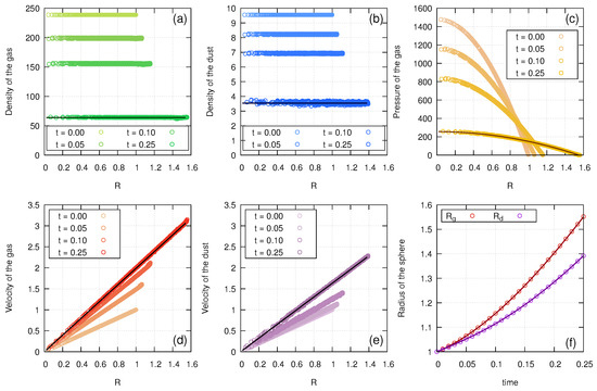
Figure 2.
Expansion of a gas and dust ball into a vacuum, model M with and moderate relaxation time (). The points show the computed values at four time moments , , , and , the solid bold line is the analytical solution at the final time . The panels represent (from left to right and from top to bottom): gas density (a), dust density (b), gas pressure (c), gas velocity (d), dust velocity (e), and radii of the gas and dust balls, respectively (f).
It is seen in Figure 2b that, at the final time moment, the density of the dust ball is more contaminated with numerical noise compared to the dust density at earlier moments, and to the gas density at the final moment. On the other hand, the observable noise level is rather acceptable considering the coarse spatial resolution used. Besides that, the design specifics of the IDIC method prescribes the use of value from (41) in the calculation of dust and gas velocities, rather than the dust density computed from (36) and presented in Figure 2. Therefore the inaccuracy in the dust density calculation does not contribute to the noise contamination in the computation of gas and particles velocities, which can be seen in Figure 2d,e. To control the numerical noise of the SPH-IDIC method, the dispersion properties of this method will be analyzed in the following work.
4.3. Ball Expansion into Vacuum at Infinitely Small and Infinitely Large Velocity Relaxation Times
Let us show now that the devised solution can be reproduced in numerical simulations with extreme relaxation times. An infinitely large relaxation time corresponds to the frozen equilibrium mode with no drag between phases. An infinitely small relaxation time corresponds to the mode of relaxation equilibrium when the drag force is so large that the gas and dust propagate jointly as an integral medium.
First, we compute the expansion of a gas and dust ball according to model L with until the time moment . The simulation results are shown in Figure 3. The notations are the same as in the previous Figure 2. In Figure 3a,b it is seen that the gas and dust densities in the L model are uniform at all times, and the radial velocity of each phase depends on the radius linearly. At the reference time point , the numerical values coincide with the analytical solutions for all macro parameters of the gas and dust cloud. It follows from Figure 3e,f that the dust ball is not affected by any forces, its center is at rest, and the dust particles of the cloud expand straight and with constant velocity. This means that frozen equilibrium conditions truly take place in model L at the times involved. The propagation of the gas ball material is affected by the pressure gradient, therefore it expands with acceleration (see the left and right panels in the second row). The comparison of the panels (f) in Figure 2 and Figure 3 shows that the gas balls expand with comparable velocities in models M and L. This is explained by the fact that the drag is almost absent in model L, and the mass content of the dust in model M is too small to exert a considerable impact on the momentum of the gas ball. However, dust balls expand with different velocities in models M and L. This is explained by the fact that, in the M model, the dust is dragged by the gas matter, so that the dust expansion velocity is higher in model M compared to model L.
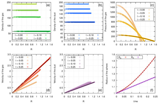
Figure 3.
Expansion of a gas and dust ball into vacuum, model L with and long relaxation time (). The points show the computed values at four time moments , , , and , the solid bold line is the analytical solution at the final time . The panels represent (from left to right and from top to bottom): gas density (a), dust density (b), gas pressure (c), gas velocity (d), dust velocity (e), and radii of the gas and dust balls, respectively (f).
Now we compute the expansion for the configuration of model S with until the same time moment . The simulation results are shown in Figure 4 with the same legend as for Figure 2. From Figure 4e it is obvious that relaxation equilibrium conditions truly take place in model S, since the gas and dust ball radii coincide during the entire simulation. The panels (a), (b), (d), and (e) show that the gas and dust ball expands into vacuum in model S similarly as in M and L, with uniform densities and linear velocities maintained at all times. In the final time moment , the computed values coincide with those from the analytical solution for all macro parameters of the gas and dust medium. This means that the IDIC method provides a high accuracy in 3D simulations of the interphase interaction in dense mixtures even if the conditions (45) and (46) fail. We note that previously, a three-dimensional model of gas and dust ball expansion with relaxation equilibrium was simulated using the SPH-IDIC method in [40,42]; however, no benchmark solution was provided for the simulated configuration to evaluate the quality of the results.
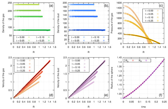
Figure 4.
Expansion of a gas and dust ball into vacuum, model S with and short relaxation time (). The points show the computed values at four time moments , , , and , the solid bold line is the analytical solution at the final time . The panels represent (from left to right and from top to bottom): gas density (a), dust density (b), gas pressure (c), gas velocity (d), dust velocity (e), and radii of the gas and dust balls, respectively (f).
The spatial distribution of gas and dust SPH particles is shown in Figure 5 and Figure 6. The expansion of the gas–dust sphere is clearly visible, while the Cartesian uniformity of the distribution of particles is preserved. The color shows the pressure in gas particles and the velocity in dust particles.
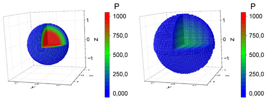
Figure 5.
The 3D distribution of gas SPH particles with and short relaxation time (model S) at two time moments and .
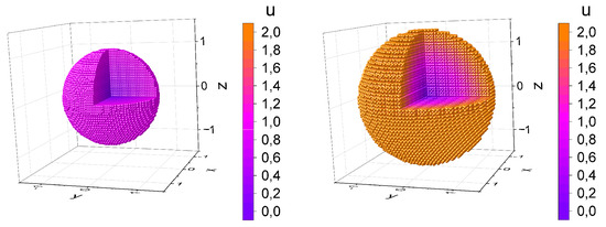
Figure 6.
The 3D distribution of dust SPH particles with and short relaxation time (model S) at two time moments and .
Furthermore, the comparison of panels (f) in Figure 3 and Figure 4 shows that the ball in the relaxation equilibrium state expands slower compared to the gas ball under frozen equilibrium conditions. This dependence correlates with a known behavior of propagating sound waves in a gas and dust material. Under relaxation equilibrium conditions, the group velocities of plane waves in the pure gas and in the gas and dust mixture are related as
This expression indicates that waves in a mixture propagate slower compared to a pure gas. Let us note that the corresponding factor is present in Equation (19) under relaxation equilibrium, since it turns out in this case .
4.4. Discussion, Results and Limits of the Study and Future Plans
In this paper, we have drawn a spherically symmetric solution for the problem of gas and dust ball expansion into vacuum. The problem was set for a system of two-fluid dynamics equations for a two-phase medium (1). For the gas–vacuum boundary, kinematic (8) and dynamic (17) conditions were defined, while for the dust ball boundary only the kinematic condition was set. The derived solution satisfies the specific initial conditions where the gas and dispersed phase densities are uniform across the space, the velocities of gas and the dispersed phase depend linearly on the radii and the dispersed phase pressure is a quadratic function of the radius. As far as it is known to the authors, no field measurements have been conducted to date that would validate the use of the two-phase fluid dynamics model for such a problem setting.
Nevertheless, considering the specific numerical simulation of ultradispersed medium dynamics, the derived solution is of interest for numerical code verification. A verification benchmark would help demonstrate that numerical methods of solving two-phase fluid dynamics equations (in the form of (1), (34), or another) may represent the analytical solution with an appropriate accuracy. Since the solution is presented for the first time, it needs to be carefully proved before it is recommended as a benchmark. In this paper, besides deriving it from the initial equations, as presented in Section 2.2, the following steps were performed to validate the solution. In Section 2.4 we show that a specific case of the derived solution correlates to a specific case of the known solution for the problem of gas ellipsoid expansion into vacuum suggested by other authors [30]. In Section 4.2 and Section 4.3 the values of the problem parameters are provided for which the derived solution is proved to be reproducible by numerical models. The numerical method used to reproduce the solution as well as its software implementation was developed by the authors of this paper. In the light of increased interest in the simulation of gas dispersion medium dynamics, we hope that this solution will be numerically reproduced in the nearest future by other authors using various numerical methods.
A promising development of this research would be a derivation of such benchmark solutions for the expansion of a two-fluid gas dispersion medium into a vacuum with no drag force discontinuity at the dust cloud boundary, as well as with no spherical symmetry requirement. It should be noted that a solution to the problem of the interpenetration of two separate fluids is known where the dispersed phase has its own pressure and buoyancy [43].
5. Conclusions
We introduced here the derivation of an analytical solution for the problem of spherically symmetric expansion of a gas and dust ball into a vacuum. A ball containing both gas and dust particles is modeled as a two-phase continuum with different velocities. The carrier phase in the system is a non-viscous and non-heat-conducting gas, and the dispersed phase represents a cloud of monodisperse particles with negligible volume. The carrier phase is described by the Euler equations and the dispersed phase by equations of continuity and motion of compressible gas without intrinsic pressure. The carrier and dispersed phases exchange momentum, and the exchange rate is described by the velocity relaxation time. The derived solution describes specific expansion conditions where radial velocities of the gas and dispersed phases depend linearly on the radii and the density of each phase is uniform across the space. The solution to the expansion problem with linear velocity and uniform density is derived for arbitrary relaxation time; hence, it extends the previously known solution into a more general case.
It is shown that the obtained solution is well reproduced in three-dimensional simulations at infinitely large, moderate, and infinitely small values of velocity relaxation time. The numerical simulations were performed with the SPH-IDIC method implemented in the open-source OpenFPM library. We suggest a practical use of this solution as a verification benchmark for computational flow dynamics models and investigating the properties of numerical methods. For convenience, we make the benchmark solution generator designed in the environment available to the public.
Author Contributions
Conceptualization, O.P.S.; software, V.V.G., A.N.S. and N.V.S.; validation, M.N.D.; formal analysis, O.P.S.; investigation, V.V.G.; writing—original draft preparation, O.P.S., A.N.S., M.N.D. and N.V.S.; writing—review and editing, O.P.S.; visualization, V.V.G. and M.N.D. All authors have read and agreed to the published version of the manuscript.
Funding
This research was funded by the Russian Science Foundation, grant number 19-71-10026.
Institutional Review Board Statement
Not applicable.
Informed Consent Statement
Not applicable.
Data Availability Statement
The benchmark solution generator and the source code of the SPH-IDIC implementation are available by https://github.com/MultiGrainSPH/OneDustBall_Scilab_OpenFPM (Accessed on 16 December 2021).
Acknowledgments
The authors are grateful to Valeriy Snytnikov for his insightful comments on the reported work.
Conflicts of Interest
The authors declare no conflict of interest.
References
- Gidaspow, D. Multiphase Flow and Fluidization: Continuum and Kinetic Theory Descriptions; Academic Press: San Diego, CA, USA, 1994. [Google Scholar]
- Marchisio, D.L.; Fox, R.O. Computational Models for Polydisperse Particulate and Multiphase Systems; Cambridge University Press: Cambridge, UK, 2013. [Google Scholar]
- Nigmatullin, R.I. Dynamics of Multiphase Media; Hemisphere Publ. Corp: New York, NY, USA, 1990; Volume 1. [Google Scholar]
- Soo, S.L. Particulates and Continuum: Multiphase Fluid Dynamics; CRC Press: Boca Raton, FL, USA, 1989. [Google Scholar]
- Akimkin, V.V.; Vorobyov, E.I.; Pavlyuchenkov, Y.N.; Stoyanovskaya, O.P. Gravitoviscous protoplanetary discs with a dust component–IV. Disc outer edges, spectral indices, and opacity gaps. Mon. Not. R. Astron. Soc. 2020, 499, 5578–5597. [Google Scholar] [CrossRef]
- Nakagawa, Y.; Sekiya, M.; Hayashi, C. Settling and growth of dust particles in a laminar phase of a low-mass solar nebula. Icarus 1986, 67, 375–390. [Google Scholar] [CrossRef]
- Takeuchi, T.; Lin, D.N.C. Radial Flow of Dust Particles in Accretion Disks. Astrophys. J. 2002, 581, 1344–1355. [Google Scholar] [CrossRef]
- Benítez-Llambay, P.; Krapp, L.; Pessah, M.E. Asymptotically Stable Numerical Method for Multispecies Momentum Transfer: Gas and Multifluid Dust Test Suite and Implementation in FARGO3D. Astrophys. J. Suppl. Ser. 2019, 241, 25. [Google Scholar] [CrossRef]
- Dipierro, G.; Laibe, G.; Alexander, R.; Hutchison, M. Gas and multispecies dust dynamics in viscous protoplanetary discs: The importance of the dust back-reaction. Mon. Not. R. Astron. Soc. 2018, 479, 4187–4206. [Google Scholar] [CrossRef]
- Marble, F.E. Dynamics of Dusty Gases. Annu. Rev. Fluid Mech. 1970, 2, 397–446. [Google Scholar] [CrossRef]
- Laibe, G.; Price, D.J. DUSTYBOX and DUSTYWAVE: Two test problems for numerical simulations of two-fluid astrophysical dust-gas mixtures. Mon. Not. R. Astron. Soc. 2011, 418, 1491–1497. [Google Scholar] [CrossRef]
- Markelova, T.V.; Arendarenko, M.S.; Isaenko, E.A.; Stoyanovskaya, O.P. Plane Sound Waves of Small Amplitude in a Gas-Dust Mixture with Polydisperse Particles. J. Appl. Mech. Tech. Phys. 2021, 62, 663–672. [Google Scholar] [CrossRef]
- Stoyanovskaya, O.P.; Grigoryev, V.V.; Savvateeva, T.A.; Arendarenko, M.S.; Isaenko, E.A.; Markelova, T.V. DMulti-fluid dynamical model of isothermal gas and buoyant dispersed particles: Monodisperse mixture, ben solution of DustyWave problem as test for CFD-solvers, effective sound speed for high and low mutual drag. Int. J. Multiph. Flow. accepted.
- Booth, R.A.; Sijacki, D.; Clarke, C.J. Smoothed particle hydrodynamics simulations of gas and dust mixtures. Mon. Not. R. Astron. Soc. 2015, 452, 3932–3947. [Google Scholar] [CrossRef][Green Version]
- Laibe, G.; Price, D.J. Dusty gas with smoothed particle hydrodynamics -I. Algorithm and test suite. Mon. Not. R. Astron. Soc. 2012, 420, 2345–2364. [Google Scholar] [CrossRef]
- Stoyanovskaya, O.P.; Davydov, M.N.; Arendarenko, M.S.; Isaenko, E.A.; Markelova, T.V.; Snytnikov, V.N. Fast method to simulate dynamics of two-phase medium with intense interaction between phases by smoothed particle hydrodynamics: Gas-dust mixture with polydisperse particles, linear drag, one-dimensional tests. J. Comput. Phys. 2021, 430, 110035. [Google Scholar] [CrossRef]
- Lehmann, A.; Wardle, M. Two-fluid dusty shocks: Simple benchmarking problems and applications to protoplanetary discs. Mon. Not. R. Astron. Soc. 2018, 476, 3185–3194. [Google Scholar] [CrossRef]
- Youdin, A.N.; Goodman, J. Streaming instabilities in protoplanetary disks. Astrophys. J. 2005, 620, 459. [Google Scholar] [CrossRef]
- Bai, X.-N.; Stone, J.M. Particle-gas Dynamics with Athena: Method and Convergence. Astrophys. J. Suppl. Ser. 2010, 190, 297–310. [Google Scholar] [CrossRef]
- Keller, J.B. Spherical, cylindrical and one-dimensional gas flows. J. Quart. Appl. Math. 1956, 14, 171–184. [Google Scholar] [CrossRef][Green Version]
- Sedov, L.I. On the integration of the equations of one-dimensional gas motion. Dokl. Akad. Nauk USSR 1953, 90, 735. [Google Scholar]
- Ovsyannikov, L. New solution of hydrodynamic equations. Dokl. Akad. Nauk 1956, 111, 47. [Google Scholar]
- Zeldovich, Y.B.; Raizer, Y.P. Physics of Shock Waves and High-Temperature Hydrodynamic Phenomena; Academic Press: New York, NY, USA, 1966. [Google Scholar]
- Nemchinov, I.V. Expansion of a Triaxial Gas Ellipsoid in a Regular Mode. Prikl. Mat. Mekh. 1965, 29, 926–929. [Google Scholar]
- Dyson, F.J. Dynamics of a Spinning Gas Cloud. J. Math. Mech. 1968, 18, 91–101. [Google Scholar] [CrossRef]
- Bogoyavlensky, O. Methods in the Qualitative Theory of Dynamical Systems in Astrophysics and Gas Dynamics; Springer: Berlin, Germany, 1985. [Google Scholar]
- Lidov, M.L. Exact solution of the equations of one-dimensional unsteady gas motion taking into account Newtonian gravitational forces. Dokl. Akad. Nauk USSR 1954, 97, 409–410. [Google Scholar]
- Bizyaev, I.A.; Borisov, A.V.; Mamaev, I.S. Figures of equilibrium of an inhomogeneous self-gravitating fluid. Celestial Mech. Dyn. Astron 2015, 122, 1–26. [Google Scholar] [CrossRef][Green Version]
- Borisov, A.V.; Kilin, A.A.; Mamaev, I.S. The Hamiltonian dynamics of self-gravitating liquid and gas ellipsoids. Regul. Chaotic Dyn. 2009, 14, 179–217. [Google Scholar] [CrossRef]
- Giron, J.F.; Ramsey, S.D.; Baty, R.S. Nemchinov–Dyson solutions of the two-dimensional axisymmetric inviscid compressible flow equations. Phys. Fluids 2020, 32, 127116. [Google Scholar] [CrossRef]
- Monaghan, J.J. Smoothed particle hydrodynamics. Rep. Prog. Phys. 2005, 68, 1703. [Google Scholar] [CrossRef]
- Stoyanovskaya, O.P.; Glushko, T.A.; Snytnikov, N.V.; Snytnikov, V.N. Two-fluid dusty gas in smoothed particle hydrodynamics: Fast and implicit algorithm for stiff linear drag. Astron. Comput. 2018, 25, 25–37. [Google Scholar] [CrossRef]
- Lorén-Aguilar, P.; Bate, M.R. Two-fluid dust and gas mixtures in smoothed particle hydrodynamics: A semi-implicit approach. Mon. Not. R. Astron. Soc. 2014, 443, 927–945. [Google Scholar] [CrossRef]
- Lorén-Aguilar, P.; Bate, M.R. Two-fluid dust and gas mixtures in smoothed particle hydrodynamics II: An improved semi-implicit approach. Mon. Not. R. Astron. Soc. 2015, 454, 4114–4119. [Google Scholar] [CrossRef]
- Monaghan, J.J.; Kocharyan, A. SPH simulation of multi-phase flow. Comput. Phys. Commun. 1995, 87, 225–235. [Google Scholar] [CrossRef]
- Monaghan, J.J. On the integration of the SPH equations for a dusty fluid with high drag. Eur. J. Mech. -B/Fluids 2020, 79, 454–462. [Google Scholar] [CrossRef]
- Price, D.J.; Laibe, G. A solution to the overdamping problem when simulating dust-gas mixtures with smoothed particle hydrodynamics. Mon. Not. R. Astron. Soc. 2020, 495, 3929–3934. [Google Scholar] [CrossRef]
- Morris, J.P.; Fox, P.J.; Zhu, Y. Modeling low reynolds number incompressible flows using sph. J. Comput. Phys. 1997, 136, 214–226. [Google Scholar] [CrossRef]
- Incardona, P.; Leo, A.; Zaluzhnyi, Y.; Ramaswamy, R.; Sbalzarini, I.F. OpenFPM: A scalable open framework for particle and particle-mesh codes on parallel computers. Comput. Phys. Commun. 2019, 241, 155–177. [Google Scholar] [CrossRef]
- Grigoryev, V.; Stoyanovskaya, O.; Snytnikov, N. Supercomputer model of dynamical gas-and-dust with intense momentum transfer between phases based on OpenFPM library. J. Phys. Conf. Ser. Accept. 2021, 2099, 012056. [Google Scholar] [CrossRef]
- Mentiplay, D.; Price, D.J.; Pinte, C.; Laibe, G. A smoothed particle hydrodynamics algorithm for multigrain dust with separate sets of particles. Mon. Not. R. Astron. Soc. 2020, 499, 3806–3818. [Google Scholar] [CrossRef]
- Davydov, M.N.; Stoyanovskaya, O.P.; Glushko, T.A. Numerical modelling of a gas-dust sphere scattering by SPH-IDIC method. J. Phys. Conf. Ser. 2020, 1675, 012071. [Google Scholar] [CrossRef]
- Panov, A.V. Invariant solutions and submodels in two-phase fluid mechanics generated by 3-dimensional subalgebras: Barochronous flows. Int. J. Non-Linear Mech. 2019, 116, 140. [Google Scholar] [CrossRef]


Publisher’s Note: MDPI stays neutral with regard to jurisdictional claims in published maps and institutional affiliations. |
© 2022 by the authors. Licensee MDPI, Basel, Switzerland. This article is an open access article distributed under the terms and conditions of the Creative Commons Attribution (CC BY) license (https://creativecommons.org/licenses/by/4.0/).