Experimental Techniques against RANS Method in a Fully Developed Turbulent Pipe Flow: Evolution of Experimental and Computational Methods for the Study of Turbulence

Abstract

Fully developed turbulent flow in a pipe was studied by considering experimental and computational methods. The aim of this work was to build on the legacy of the University of Manchester, which is widely regarded as the birthplace of turbulence due to the pioneering work of the prominent academic Professor Osborne Reynolds (1842–1912), by capturing the evolution of fluid turbulence analysis tools over the last 100 years. A classical experimental apparatus was used to measure the mean velocity field and wall shear stress through four historical techniques: static pressure drop; mean square signals measured from a hot-wire; Preston tube; and Clauser plot. Computational Fluid Dynamics (CFD) was used to simulate the pipe flow, utilizing the Reynolds-averaged Navier–Stokes (RANS) method with different two-equation turbulence models. The performance of each approach was assessed to compare the experimental and computational methods. This comparison revealed that the numerical results produced a close agreement with the experiments. The finding shows that, in some cases, CFD simulations could be used as alternative or complementary methods to experimental techniques for analyzing fully developed turbulent pipe flow.

1. Introduction

Turbulence appears in the majority of the fluids existent in nature and it is important for a variety of practical engineering applications, including ventilation systems and biomedical research. A flow is characterized as turbulent when the Reynolds number exceeds a critical value. The critical Reynolds number, as well as the characteristic length, are case-specific parameters. Many environmental and industrial applications are associated with augmented Reynolds numbers which characterize the flow regime as turbulent [1].

Given its ubiquity and complexity, turbulence has been one of the most studied subjects in fluid dynamics. After more than 100 years of research, various methods for analyzing turbulent flow have been developed, but a clear understanding of their evolution has not yet emerged. The goal of this investigation was to show the evolution of fluid turbulence analysis tools by reviewing the scopes and limitations of historical techniques and by comparing common experimental and computational methods for measuring the mean velocity field and wall shear stress for turbulent flow. Considering its wide applications, this study may offer a significant starting point for analyzing fluid behavior in a vast range of contexts.

In this work, the case study used for comparing the methods was the behavior of a fully developed turbulent pipe flow. For the experimental techniques, hot-wire anemometry was used to measure the mean and fluctuating properties of a turbulent flow of air [2], which was forced to flow inside a pipe by the action of an upstream fan, while the wall shear stresses were estimated using four different methods: (a) Static pressure drop over a known length of pipe; (b) Mean square signals from a hot-wire; (c) Preston tube; and (d) The law of the wall, also known as the Clauser plot technique. The velocity and viscosity measurements were further analyzed with attention given to the distribution across the pipe. For the computational method, the commercial CFD software ANSYS Fluent (17.1, Ansys, Canonsburg, PA, USA) was used to numerically simulate the turbulent flow in the pipe, utilizing a two-equation eddy-viscosity turbulence model [3]. By comparing the experimental data against the CFD results, this study provided an assessment of the performance of historic experimental techniques with one of the most popular computational simulations, demonstrating from a practical perspective the evolution of methods available for a fluid dynamicist studying the complex phenomena involved in turbulent flows.

Evolution of the Experimental and Computational Techniques

Experimental techniques have been used to study turbulent flows for many decades. The experimental work of Reynolds in the late 19th century at the University of Manchester contextualized the parameters associated with turbulent flows [4]. A substantial number of studies have specifically examined turbulent pipe flows and it is important to note the evolution of these methods over time. The static pressure drop method, based on the fundamental theory of fluid mechanics, has been applied for the wall shear stress calculation since the introduction of pressure tapping techniques in 1888 [5]. Hot-wire anemometry was introduced at the beginning of the 20th century, drawing on the theoretical work of Boussinesq and Russel, although the first actual experiments were not conducted until the 1910s, most notably in the work of King [6,7,8]. Subsequent research on the measurement of fluctuating turbulent velocity with hot-wires enabled the application of hot-wire anemometry for the calculation of the wall shear stresses [9,10]. In 1954, Preston developed a new approach based on the principle that the surface shear stress could be accurately predicted using modified Pitot tubes of different sizes [11,12]. Finally, the law of the wall, also known as the Clauser plot technique, was introduced in 1956, offering a graphic approach for approximating the wall shear stress [13,14].

Since 1969, computational techniques have discretized the Navier–Stokes equations in space and time in order to investigate turbulent effects [15]. Due to the very fine structures associated with turbulent flows, the analytical solution offered by the Navier–Stokes equations was hardly feasible [16], although it is worth noting that fine turbulent structures may be of low interest in many applications. Approximation models have been developed for the estimation of turbulent flow fields [17,18,19]. The first computational technique examining turbulence was the Large Eddy Simulation (LES), introduced in 1970 by Deardorff. In 1972, Orszag and Patterson developed the first Direct Numerical Simulation (DNS) for low Reynolds number [20]. Despite their high level of detail, these simulations were limited in terms of their utility because they required supercomputers and their computational times were excessively long for everyday applications [21]. Launder and Spalding presented the Reynolds-averaged Navier–Stokes (RANS) method in 1972, which later became the most common technique for modelling turbulence [22]. Its improved efficiency has made the RANS method the standard tool for turbulence modelling for most engineering applications, even up to the present day [23,24,25,26,27,28,29].

2. Materials and Methods

In this section, the experimental set-up and the techniques which were applied to measure the velocity field and wall shear stress of a fully developed flow in a pipe are described, while the computational method and the key parameter settings which were used to simulate the turbulent pipe flow are outlined.

2.1. Experimental Set-Up

The classical experimental apparatus which was designed to compare four historical techniques for measuring the velocity field and wall shear stress of a fully developed pipe flow was located in the premises of the University of Manchester (Manchester, UK) and set up as shown in Figure 1.

This experimental set-up consisted of:

• A brass pipe with length to diameter ratio of 125:1, which was considered an adequate ratio for a high Reynolds number.
• A variable speed centrifugal fan, which was used at the inlet and forced air at ambient conditions to flow along the pipe.
• An analogue manometer, which was connected via a pressure switch to static pressure tapings in the wall of the pipe and also to a Preston tube placed at the pipe exit.
• A Preston tube, which was used at the outlet of the brass pipe to measure the dynamic pressure.
• Static pressure tappings, which were used at two points on the wall of the pipe to calculate the pressure drop along the pipe over a fixed distance.
• A set of two pressure switches, which were used to interconnect a digital manometer apparatus with the Preston tube.
• A hot-wire anemometer.

2.2. Instrumentation and Measurements

2.2.1. Anemometry Measuring System

The anemometry measuring system consisted of:

• Two single hot-wire probes (one straight and one 45° hot-wire).
• A set of traverse gears, which were implemented to move the hot-wire to the required position in the pipe.
• Two Constant Temperature Anemometer (CTA) bridges.
• A linearizer, which was used to enhance the non-linear behavior of the amplifier and to filter down a portion of the noise interfering with the output data from hot-wire anemometry, mainly caused by the fluctuation of the probe in the pipe.
• Two separate digital voltage meters, which measured the mean and the Root Mean Square (RMS) velocities.
• AC amplifier, which was used to increase the signal of the time-varying voltage.

2.2.2. Hot-Wire Anemometer

Hot-wire anemometers have been widely used to measure flow velocities, especially those with high frequency velocity fluctuations, i.e., turbulence [30]. A hot-wire anemometer consists of a sensor used to measure the change of velocities rapidly with good spatial and time resolution and comprises a metallic (usually tungsten) filament of a micron in diameter [31] that has a known and constant variation of resistance with temperature. This filament is welded to metallic prongs of much larger diameter and the filament length is typically of the order of 2–3 mm long, depending on the probe design. When used, the hot-wire probe is placed in air streams and heated by passing a small electric current through it and some of the heat generated by Joule effect in the filament is absorbed by the air flow via convection [32]. This cooling effect changes the resistance of the wire and thus provides a means of measuring the flow; the change of resistance reflects the flow velocity. There are two main types of hot-wire anemometer, the constant current (CCA) and constant temperature (CTA), and the latter is more common. In operation, the CCA is continuously cooled by the flow, and this ultimately leads to the sensitivity decreasing as the wire temperature approaches ambient at high velocities. With the CTA, there is a servo electrical system consisting of a Wheatstone bridge that responds to the change of resistance of the hot-wire by either increasing or decreasing the power to it, according to whether it is too cold (high velocity) or too hot (low velocity) [33]. This change of power is measured as a change of voltage that can be directly related to the flow velocity by suitable calibration [32]. It is essential that the hot-wire does not make contact with the pipe wall, as this renders it ineffectual; it has been observed that the hot-wire measurements near to the wall increase the zero volts and any subsequent measurement produces an error [34] and that the hot-wire is shorted out if both prongs touch the wall. The hot-wire probes used in this experiment were an Analogue to Digital Converter (ADC) and a computer control, which allowed fluctuations in time to be recorded from the sensor.

2.3. Experimental Procedure

The variable speed fan forced a flow of air at ambient conditions through a horizontal tube of circular cross section. The tube measured 12.75 m long. The mass flow rate was controlled through the opening and closing of the inlet, which determined the air intake to produce turbulent flow, corresponding to a Reynolds number >55,000. The measuring section was located close to the pipe outlet, where the flow can be considered fully developed, and the pressure drop in the air flow along the pipe was obtained from two pressure sensors. A Preston tube was attached at the exit of the pipe to measure the wall shear stress. A hot-wire anemometer for measuring the local air flow velocity was mounted on a transverse gear that allowed the placement of the hot-wire along a diametral line from a position of 0.1 mm from the pipe wall until the pipe centerline, measuring the mean and root-mean-square (rms) velocity profile at each location.

2.3.1. Measurement of the Velocity Field

The hot-wire was positioned so that measurements of the mean and RMS velocities could be appropriately acquired from a distance as close to the wall as possible using the digital voltmeters. The only way to ensure positional accuracy was to connect a voltmeter to measure the resistance between the hot-wire and the brass tube. The contact between them meant that this was at the wall (i.e., 0 mm). Preliminary measurements were taken from an initial distance of 0.1 mm from the wall and several subsequent measurements were taken along the radius of the tube up to the centerline. This enabled the average Reynolds number, which determines the regime of the flow in the pipe, to be calculated. Usually, without using the linearizer, the calibration follows King’s law [35]:

$$E^2=A+B{u}^n$$

(1)

where E is the voltage along the hot-wire, u is the velocity of the normal flow of the wire, and A, B and n are constants. In this experiment, the straight hot-wire was pre-calibrated with a linear calibration coefficient $k_{hw}$ equal to $0.5 \mathrm{V}/{\mathrm{ms}}^{-1}$ applied to the hot-wire output. The calibration coefficient is non-linear; however, here, a linear slope was assumed, meaning that, to calculate the velocity components, the readings from the voltmeter needed to be multiplied by a factor of two. The required velocities were obtained as follows:

$$\overline{U}=\overline{E_{ac}}\frac{1}{k_{hw}}$$

(2)

$$U_{rms}=E_{rms}\frac{1}{k_{hw}}$$

(3)

$$U=\overline{U }+U_{rms}$$

(4)

where $\overline{U}$ is the mean velocity, $E_{ac}$ is the mean voltage alternating current, $E_{rms}$ is the root mean square voltage, $U$ is the total velocity, and $U_{rms}$ is the root mean square velocity. Equation (4) adopted the Reynolds decomposition, which represents the instantaneous velocity as a summation of the mean (time-averaged) velocity and the fluctuating velocity. The convention of associating the x-axis with the mean velocity and y-axis with the direction traverse to the supports was used to represent the velocity. Thus, to verify this condition, it was necessary to initially calculate the Reynolds number using the non-dimensional Reynolds equation:

$$Re=\frac{\rho U{D}_{pipe}}{\mu }$$

(5)

where $Re$ is the Reynolds number and $\mu$ is dynamic viscosity.

The distribution of the velocity profile gave a reliable illustration of the main features of the turbulent flow and could be compared with the data collected in experiments utilizing dimensionless analysis. Dimensionless velocities indicated that there was a general solution of the velocity profile applicable for all fluids and was calculated as follows:

$$U^{+}=\frac{U}{U_{\tau }}$$

(6)

where $U^{+}$ is the dimensionless velocity and $U_{\tau }$ is the shear velocity. The shear velocity was defined as:

$$U_{\tau }=\sqrt{\frac{{\tau }_w}{\rho }}$$

(7)

where ${\tau }_w$ is the wall shear stress and $\rho$ is the density. The dimensionless near wall distance $Y^{+}$ was defined as:

$$Y^{+}=\frac{y{U}_{\tau }}{\nu }$$

(8)

where $y$ is the distance to the nearest wall and $\nu$ is the kinematic viscosity.

2.3.2. Power-Law Velocity Profile

The power-law velocity profile is used to represent the turbulent flow in a pipe. The empirical relation was obtained as:

$$\frac{\overline{U}}{U_m}={\left(1-\frac{r}{R}\right)}^{\frac{1}{n}}$$

(9)

where $U_m$is the maximum velocity at the centerline, $r$ is the distance from the pipe center, $R$ is the total radius of the pipe, in this case $R=51 \mathrm{mm}$, and n is a constant exponent that depends on the Reynolds number. The empirical one-seventh power-law declares that the value of the power law exponent $n$ approximates most of the flows with the value of 7 [36].

2.3.3. Method 1: Static Pressure Drop

The static pressure drop method, available for fully developed internal flows and axisymmetric conditions, was used to quantify the average wall shear stress from the axial pressure gradient. The pressure drop was measured with the use of two static pressure tappings along the pipe. The shear stress ${\tau }_w{}_{PD}$ for a fully developed circular pipe acting over a surface area $A$ is related with the pressure drop $\mathsf{\Delta }P$ over a distance between static tapping points $L$ of a constant cross-sectional area $A_c$ by:

$${{\displaystyle \int }}_A^{}{\tau }_{w_{PD}} dA=\Delta P{A}_c$$

(10)

$${\tau }_{w_{PD}}=\frac{\Delta P\pi R^2}{2\pi RL}=\frac{\Delta P}{2L}R$$

(11)

Harotinidis suggested that this method is the most reliable for analyzing fully developed internal flows with axisymmetric conditions [37]. However, its utility is limited because only flows in a circular pipe meet these conditions and, even for these flows, this method can affect the accuracy of the measurement, due to factors such as the size of the pressure tap and the quality of the tap hole [38].

2.3.4. Method 2: Mean Square Signal (45° Hot-Wire)

The slanted hot-wire is sensitive to the components of the velocity fluctuation of turbulent and/or unsteady flow. The wire orientation with respect to the mean flow vector and wire cooling laws vary the sensitivity coefficients, A. The equation that describes the heat transfer of the hot-wire can be linearized to establish a relation between the anemometer voltage fluctuation, E, and the velocity fluctuations, $u^{\prime }, v^{\prime }, w^{\prime },$ if these fluctuations are minor [38]:

$$E=A_u{u}^{\prime }+A_v{v}^{\prime }+A_w{w}^{\prime }$$

(12)

After squaring and averaging the equation, the mean value of the anemometer fluctuations can be found:

$$\overline{E^2}=A_u{}^2\overline{{u^{\prime }}^2}+A_v{}^2\overline{{v^{\prime }}^2}+A_w{}^2\overline{{w^{\prime }}^2}+2A_u{A}_v\overline{u{}^{\prime }v{}^{\prime }}+2A_u{A}_w\overline{u{}^{\prime }w{}^{\prime }}+2A_v{A}_w\overline{v{}^{\prime }w{}^{\prime }}$$

(13)

Deriving the sensitive coefficients of a slanted hot-wire and assuming steady flow and simple cooling laws, the heat transfer of a hot-wire by an effective velocity can be described by King’s law, where the slope represents the sensitivity [35]. With this method, the wall shear stress was estimated using a single 45° hot-wire in reversed horizontal attitudes, positioned half a diameter upstream of the pipe exit. The initial probe position was set to 10 mm from the wall and then traversed the diameter of the pipe towards the centerline, using pre-defined increments. A second set of measurements was taken at the same positions with the probe rotated 180°. On this occasion, the probe traversed the diameter of the pipe from the centerline towards the wall until it reached the distance of 10 mm from the wall. The RMS voltages were measured with the 45° hot-wire, which translated the RMS velocities. The two traverses in the horizontal plane, $E_1$ and $E_2$, corresponded to the instantaneous output voltage applied across the hot-wire [33]:

$$\overline{u{}^{\prime }v{}^{\prime }}=\frac{E_2^2-E_1^2}{2k_{hw}^2}$$

(14)

where $\overline{u{}^{\prime }v{}^{\prime }}$ represents the time average of the product of the fluctuating velocity components $u{}^{\prime }$ and $v{}^{\prime }$ and has the dimension of velocity squared, and where $k_{hw}$ is the calibration coefficient. Due to the eddy motion of the particles of the fluid, the Reynolds shear stress ${\tau }_{xy}^{\prime }$ can be interpreted as the shear force per unit area and, to calculate the wall shear stress, the following equation was used:

$${\tau }_{xy}^{\prime }=\rho \overline{u{}^{\prime }v{}^{\prime }}$$

(15)

The boundary conditions applied at the wall were: ${\left(\overline{u^{\prime }{v}^{\prime }}\right)}_{wall}=0$ and $k_{wall}=0$. Based on McDonough’s work demonstrating that the shear stress $\tau$ is a linear function of the variable radius r by the pipe radius $R$ and the wall shear stress [36], the value of the shear stress can also be obtained through:

$$\tau = {\tau }_w\frac{r}{R}$$

(16)

2.3.5. Method 3: Preston Tube

The wall shear stress was also measured using a Preston tube, positioned so that its outer surface was tangential to the pipe inner wall while facing upstream. With appropriate configuration of the analogue manometer, the dynamic pressure was taken. Theoretically, with the Preston tube, the wall shear stress is related to the dynamic pressure as:

$$\left[\frac{\rho {\tau }_w{d}^2}{{\mu }^2}\right]=f\left[\frac{\rho \Delta P{d}^2}{{\mu }^2},\frac{d}{D}\right]$$

(17)

where d and D are the internal and external diameters of the Preston tube respectively. As the Preston tube is a thick-walled tube, it tends to give the most reproducible behavior because it matches the skin friction with the data of the stagnation pressure from the tube placed at the wall. Historical tests have established relationships between the wall shear stress ${\tau }_w$ and the dynamic pressure $\mathsf{\Delta }P$, defined as the mean difference between the pressure sensed by the Preston tube and the static pressure obtained from a nearby wall tap [38]. In this case, where $\frac{d}{D}=0.6$, the following widely accepted analytical relationships were obtained [39]:

$$0<X^{*}<2.9$$

(18)

$$Y^{*}=X^{*}+0.037$$

$$2.9<X^{*}<5.6$$

(19)

$$Y^{*}=0.827-0.1381X^{*}+0.1437X^{{*}^2}-0.006 X^{{*}^3}$$

$$5.6<X^{*}<7.6$$

(20)

$$Y^{*}=2 {log}_{10}\left(1.95X^{*}+4.10\right)+X^{*}$$

where

$$X^{*}={log}_{10}\left[\frac{\rho \Delta P{d}^2}{4{\mu }^2}\right]$$

(21)

Having prescribed $X^{*}$ and determined $Y^{+}$, the wall shear stress can then be defined as:

$${\tau }_w=\frac{4 \left({10}^{Y^{*}}\right){\mu }^2}{\rho d^2}$$

(22)

2.3.6. Method 4: Clauser Plot

In turbulent flows over smooth surfaces, there is always a sub-layer next to the wall in which the flow is laminar, since a solid surface tends to damp out the turbulent fluctuations. Nevertheless, within the viscous sub-layer and the inner region, which is a fully turbulent flow region, the turbulent stress is zero. In the log-law region at the inner region, the dimensionless velocity is represented in the logarithmic form as:

$$U^{+}=\frac{1}{\kappa }\ln Y^{+}+B$$

(23)

where $\kappa$ is the Von Karman constant and is assumed, with $\kappa =0.41$, and $B=5.3$ [13,14]. This form of velocity distribution is widely used in turbulent pipe flow and is known as the “Universal Law of the Wall” [36].

The Clauser plot is a graphical method used to estimate the turbulent wall shear stress from its correlation with the law of the wall. Equation (23) can be rearranged and presented in a normalized form to obtain the wall shear stress, using the properties of the velocity profile in the logarithmic part of the boundary layer [40]:

$$\frac{U\left(r\right)}{U_{\tau }}=\frac{1}{\kappa }\ln \left(\frac{y{U}_{\tau }}{\nu }\right)+B$$

(24)

Multiplying both sides by $\frac{U_{\tau }}{U_m}$gives:

$$\frac{U\left(r\right)}{U_m}=\left[\frac{1}{\kappa }\frac{U_{\tau }}{U_m}\right]\ln \left(\frac{y{U}_m}{\nu }\right)+\left[\frac{1}{\kappa }\frac{U_{\tau }}{U_m}\ln \left(\frac{U_{\tau }}{U_m}\right)+B\frac{U_{\tau }}{U_m}\right]$$

(25)

where, as indicated previously, the friction velocity is equal to: $U_{\tau }=\sqrt{\frac{{\tau }_w}{\rho }}$ and noting that the friction coefficient is given by:

$$C_f=2{\left(\frac{U_{\tau }}{U_m}\right)}^{2 }$$

(26)

where $C_f$ is the wall skin friction coefficient. The Clauser plot equation can thus be rewritten as follows:

$$\frac{U\left(r\right)}{U_m}=\left[\frac{1}{\kappa }\sqrt{\frac{C_f}{2}}\right]\ln \left(\frac{y{U}_m}{\nu }\right)+\left[\frac{1}{\kappa }\sqrt{\frac{C_f}{2}}\ln \left(\sqrt{\frac{C_f}{2}}\right)+B\sqrt{\frac{C_f}{2}}\right]$$

(27)

where $\kappa$ and $B$ are constants and the velocity terms can be obtained from the experiment, leaving only the friction coefficient as an unknown. The value of the friction coefficient $C_f$ is estimated graphically when different values are superposed in the semi-logarithmic plot of $\frac{U}{U_m}$ vs. $\frac{U_{m}y}{\nu }$ [41], as discussed further in the Results section. Therefore, the wall shear stress can be obtained by rearranging Equation (26) and replacing the friction velocity from Equation (7):

$${\tau }_w=\frac{\rho U_m^2{C}_f}{2}$$

(28)

2.4. Computational Method

The computational approach used for simulating the turbulent pipe flow was the most popular commercial CFD package, ANSYS Fluent. Although the length of the pipe in the experiment was required to be as long as $L=125D$ to ensure a fully developed turbulent flow, the computational domain could be simplified down to a cylindrical segment of length 4 mm and diameter 102 mm, simulated using a periodic boundary condition. This significantly reduced the computational time, and also took advantage of the axisymmetric pipe.

2.4.1. Grid Generation

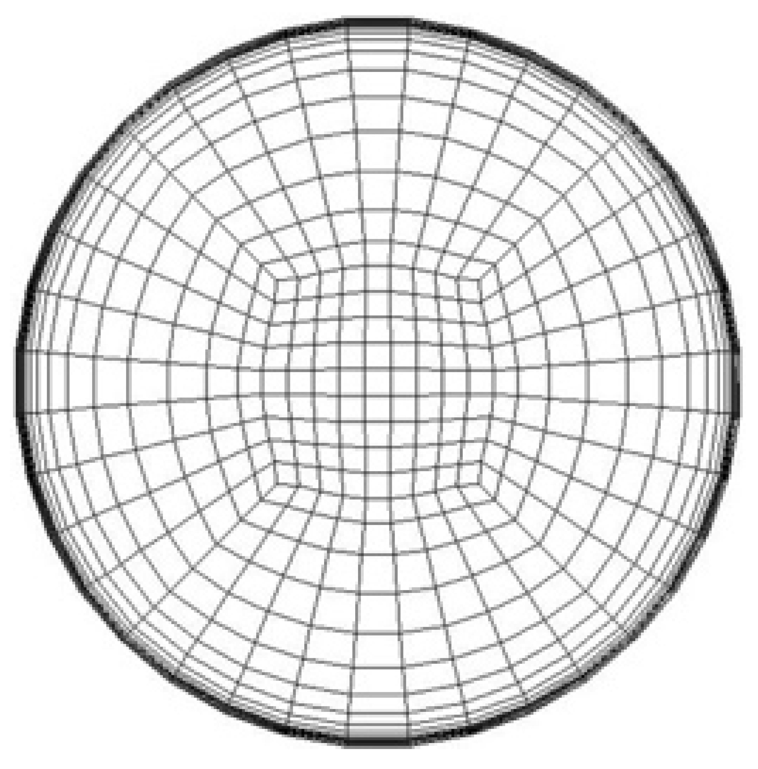
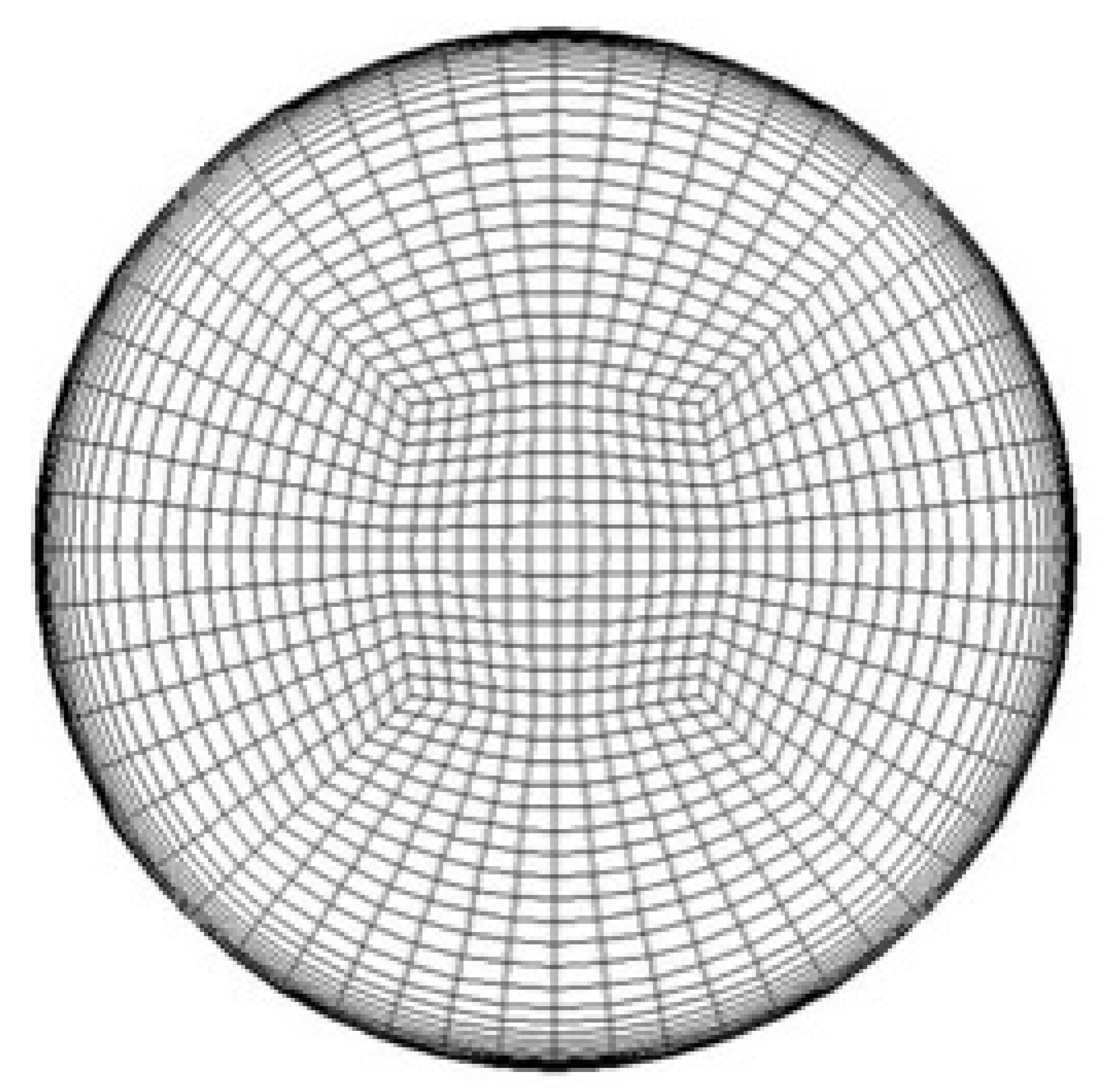
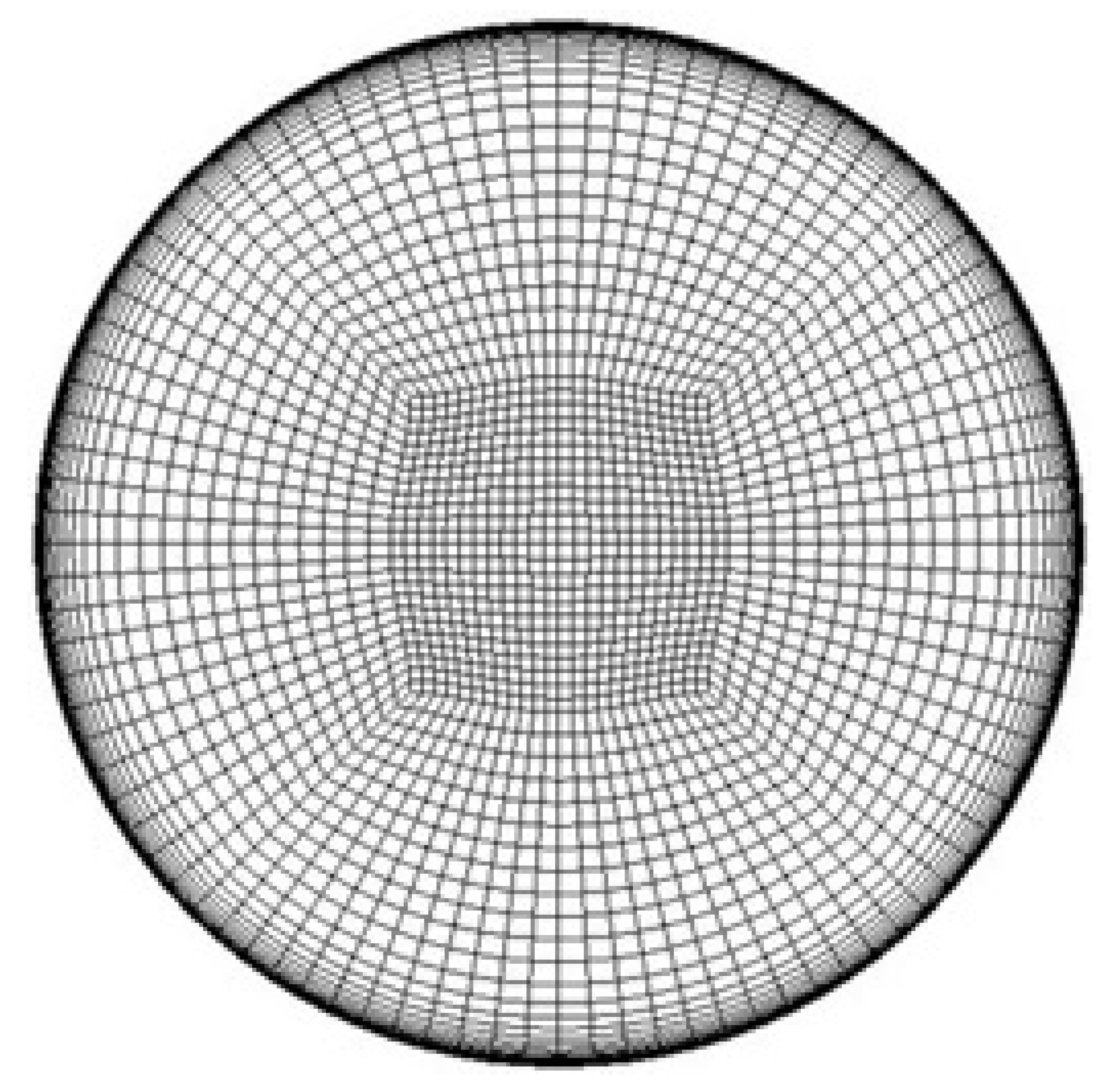
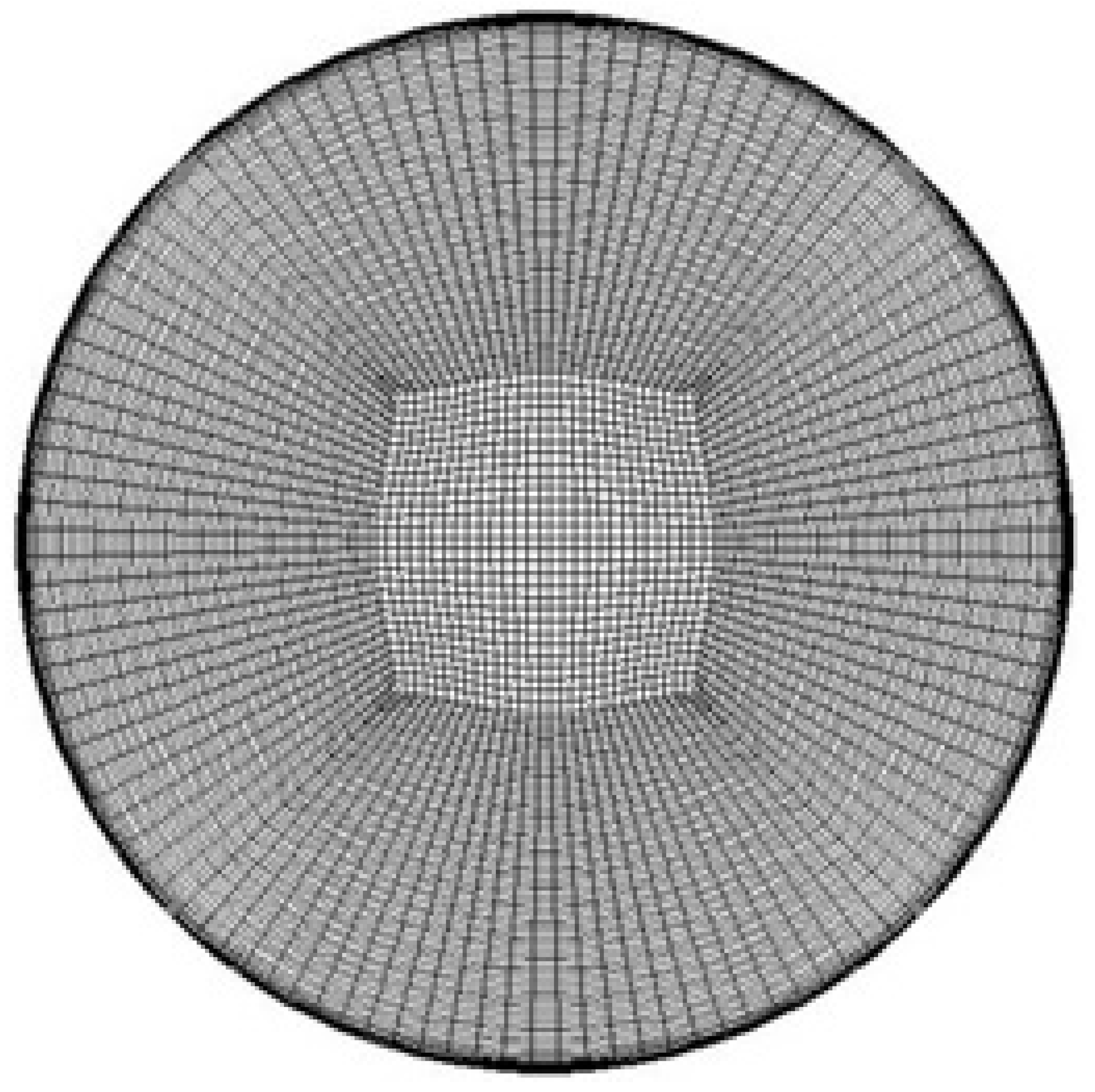
A multi-block grid was generated from the 3D circular pipe computational domain and was divided into two sub-regions: a central square region and an exterior circular region. Accurate representation of the viscous sublayer is required for a satisfactory prediction of wall-bounded turbulent fluids. The first cell height was calculated using Equation (8). The mesh must be finest around the wall and become progressively coarser towards the central square region, with an aspect ratio of 1.2. The stream-wise direction does not require an excessive number of cells. To analyze grid independency, four different grid resolutions were compared, as shown in

Table 1. Comparative table of 3D Multiblock/Hexahedral grid method.

Coarse Mesh	Medium Mesh	Fine Mesh	Very Fine Mesh
3060 cells	9520 cells	30,240 cells	90,045 cells

.

2.4.2. Turbulence Modelling

Turbulence modelling is a crucial methodological aspect of any CFD simulation and can significantly affect the final results. In theory, the Navier–Stokes equations are adequate for simulating a turbulent flow, but, due to the small size and fine detail of the turbulent structures and the consequent demand for a very fine domain discretization, the Direct Numerical Simulation (DNS) tends to be deemed computationally unaffordable. To overcome these profound limitations, turbulence models have been developed in which the eddies are approximated, either by an averaged flow field (RANS approach) or by limiting the size of the eddies which are modelled (Large Eddy Simulation [LES]). The turbulence model used to approximate the eddies by an averaged flow field in this work was the RANS method, since it is the most computationally inexpensive and offers a good representation of the flow field [29]. Several RANS models have been introduced over the last decades and applied in demanding CFD applications [42,43,44,45,46].

The two-equation turbulence models simulated and compared in this work were the standard $k-\epsilon$, $k-\omega$ and $k-\omega -SST$ models.

Standard $k-\epsilon$ Model

The $k-\epsilon$ turbulence model is the most common tool used in CFD to simulate mean flow in turbulent conditions, especially planar shear layers and recirculating fluids. This method was developed to improve the mixing-length model, adding two more equations: one for the turbulence kinetic energy k and the other for the rate of dissipation of turbulence energy ε [22].

$$\frac{\partial \left(\rho k\right)}{\partial t}+\frac{\partial \left(\rho k{u}_i\right)}{\partial x_i}=\frac{\partial }{\partial x_j}\left[\frac{{\mu }_t}{{\sigma }_k}\frac{\partial }{\partial x_j}\right]+2{\mu }_t{E}_{ij}{E}_{ij}-\rho \epsilon$$

(29)

$$\frac{\partial \left(\rho \epsilon \right)}{\partial t}+\frac{\partial \left(\rho \epsilon u_i\right)}{\partial x_i}=\frac{\partial }{\partial x_j}\left[\frac{{\mu }_t}{{\sigma }_{\epsilon }}\frac{\partial }{\partial x_j}\right]+C_{1\epsilon }\frac{\epsilon }{k}2{\mu }_t{E}_{ij}{E}_{ij}-C_{2\epsilon }\rho \frac{{\epsilon }^2}{k}$$

(30)

where $E_{ij}$ is the rate of deformation, and the eddy viscosity is represented as:

$${\mu }_t=\rho C_{\mu }\frac{k^2}{\epsilon }$$

(31)

The values of the constants are: $C_{\mu }$= 0.09, $C_{1\epsilon }$= 1.44, $C_{2\epsilon }$= 1.92, ${\sigma }_k$= 1 and ${\sigma }_{\epsilon }$= 1.3 [15].

Standard $k-\omega$ Model

In 1998, the eddy viscosity was introduced as ${\nu }_T=\frac{k}{\omega }$ with the following evolution equation of k and ω [47]:

$$\frac{\partial \left(\rho k\right)}{\partial t}+\frac{\partial \left(\rho u_{j}k\right)}{\partial x_j}=\rho P-{\beta }^{*}\rho \omega k+\frac{\partial }{\partial x_j}\left[\left(\mu +{\sigma }_k\frac{\rho k}{\omega }\right)\frac{\partial k}{\partial x_j}\right]$$

(32)

$$\frac{\partial \left(\rho \omega \right)}{\partial t}+\frac{\partial \left(\rho u_j\omega \right)}{\partial x_j}=\frac{\gamma \omega }{k}P-\beta \rho {\omega }^2+\frac{\partial }{\partial x_j}\left[\left(\mu +{\sigma }_{\omega }\frac{\rho k}{\omega }\right)\frac{\partial \omega }{\partial x_j}\right]+\frac{\rho {\sigma }_d}{\omega }\frac{\partial k}{\partial x_j}\frac{\partial \omega }{\partial x_j}$$

(33)

$$P={\tau }_{ij}\frac{\partial u_i}{\partial x_j}$$

(34)

Standard $k-\omega -SST$Model

This model is a combination of the $k-\omega$ and the $k-\epsilon$ turbulence models as proposed by Menter [48] but, in this case, the $k-\omega$ formulation was implemented in the inner region of the boundary layer and it was substituted by the $k-\epsilon$ model for the free shear region of the flow using the turbulence dissipation rate $\epsilon$. In the $k-\omega -SST$ model, the turbulent kinetic energy $k$ and the specific rate of dissipation $\omega$ are expressed through the following differential equations:

$$\frac{\partial k}{\partial t}+U_j\frac{\partial k}{\partial x_j}=P_k-{\beta }^{*}k\omega +\frac{\partial }{\partial x_j}\left[\left(\nu +{\sigma }_k{\nu }_T\right)\frac{\partial k}{\partial x_j}\right]$$

(35)

$$\frac{\partial \omega }{\partial t}+U_j\frac{\partial \omega }{\partial x_j}=\alpha S^2-\beta {\omega }^2+\frac{\partial }{\partial x_j}\left[\left(\nu +{\sigma }_{\omega }{\nu }_T\right)\frac{\partial \omega }{\partial x_j}\right]+2\left(1-F_1\right){\sigma }_{{\omega }_2}\frac{1}{\omega } \frac{\partial k}{\partial x_i} \frac{\partial \omega }{\partial x_i}$$

where the eddy viscosity, ${\nu }_T$ is expressed as:

$${\nu }_T=\frac{a_{1}k}{max\left(a_1\omega , S{F}_2\right)}$$

(36)

while

$$F_2=\mathit{tanh}\left({\left[\frac{2\sqrt{k}}{{\beta }^{*}\omega y},\frac{500v}{y^2\omega }\right]}^2\right)$$

(37)

$$P_k=\mathit{min}\left({\tau }_{ij}\frac{\partial U_i}{\partial x_j}, 10{\beta }^{*}k\omega \right)$$

(38)

$$F_1=\mathit{tanh}\left({\left[min\left(max\left[\frac{\sqrt{k}}{{\beta }^{*}\omega y^2},\frac{500 \nu }{y^2\omega }\right],\frac{4{\sigma }_{{\omega }_2}k}{C{D}_{k\omega }{y}^2}\right)\right]}^4\right)$$

(39)

$$C{D}_{k\omega }=\mathit{max}\left(2\rho {\sigma }_{{\omega }_2}\frac{1}{\omega } \frac{\partial k}{\partial x_i}\frac{\partial \omega }{\partial x_i}, {10}^{-10}\right)$$

(40)

The closure constants involved in the $\kappa -\omega -SST$ model are shown in

Table 2. Closure constants of the $k-\omega -SST$ model.

$\mathit{\kappa }-\mathit{\omega }$	$\mathit{\kappa }-\mathit{\epsilon }$	$\mathit{S}\mathit{S}\mathit{T}$
${\sigma }_{k1}=0.85$	${\sigma }_{k2}=1.00$	${\beta }^{*}=0.09$
${\sigma }_{\omega 1}=0.65$	${\sigma }_{\omega 2}=0.856$	${\alpha }_1=0.31$
${\beta }_1=0.075$	${\beta }_2=0.0828$

. The following boundary conditions for $\kappa$ and $\omega$ are set on the wall: $k_{wall}=0$ and ${\omega }_{wall}=10\frac{6v}{\beta {\left(\Delta d_1\right)}^2}$.

2.4.3. Boundary Conditions

At the entrance of the pipe, an estimated mass flow rate of $\dot{m}=7.5\times {10}^{-2}\mathrm{kg}/\mathrm{s}$ was translated into a constant velocity of $7.5\mathrm{m}/\mathrm{s}$, which was equally distributed along and normal to the inlet surface.

In the experiment, the Reynolds number was notably high at $Re=57,469$, so the assumption of a turbulent regime in the simulation was valid. A turbulence intensity of $10\%$ was also assumed at the inlet.

Periodic boundary conditions are applied when the fluid across two opposite planes of the computational domain are the same [49]. For a fully developed flow, it is not necessary to simulate the full length of the pipe so, to reduce the number of cells and the computational time, the domain simply comprised a small section of the pipe and cyclic or periodic boundary conditions were applied, meaning that the results of the outlet were the new input of the inlet. No slip-boundary conditions were applied on the pipe wall to reproduce the effects of friction with null velocity at the wall and a static pressure boundary condition of zero pascals was set at the outlet.

Table 3. Parameters for the simulation.

Parameter	Value
Pipe inner diameter	0.102 m
Length	0.004 m
Reynolds number	57,469
Air density	1.19 kg/m3
Air viscosity	1.82 × 10−5 kg/ms
Von-Karman constant	0.41 (±0.1)
Mass flow rate	7.5 × 10−2 kg/s
Velocity	7.5 m/s
Nearest wall distance	3.43 × 10−5 m

summarizes the main parameters used in the CFD simulation.

2.4.4. Discretization

The discretization of the partial derivative equations at the grid points used the Finite Volume Method (FVM). A second order discretization scheme for evaluating the convective and diffusive terms was selected to ensure that the solution remained bounded because it has been proven that higher order discretization schemes bring convergence problems and instability of the solution [50].

2.4.5. Pressure-Velocity Coupling Scheme

The Semi-Implicit Method for Pressure Linked Equations (SIMPLE) scheme, which is broadly used in CFD simulations [51,52,53], was applied in the simulation. As there is no equation for controlling the evolution of the pressure in the set of the Navier–Stokes equations, an iterative procedure was needed to relate the pressure and velocity. It is worth noting that one disadvantage of the SIMPLE scheme is that it takes more time to converge and this was evidenced in the time taken by the simulations.

2.4.6. Convergence Criteria

Due to the presence of non-linear convection terms in the momentum equations, convergence criteria in CFD need to be performed by an iterative method. A residual value was used to monitor convergence and to assess proximity to the solution. The iterations should stop when the difference between the estimated solution and the previous approximation has reached a maximum residual value. The maximum residual value settled for the simulation was 1.0 × 10⁻⁶.

3. Results and Discussion

The results of the methods which were used to examine fully developed turbulent pipe flow are presented and discussed in this section. The numerical simulation results are compared against the experimental data to assess their performance and indicate the potential utility of computational versus experimental methods.

3.1. Experimental Results: Velocity Profile Analysis

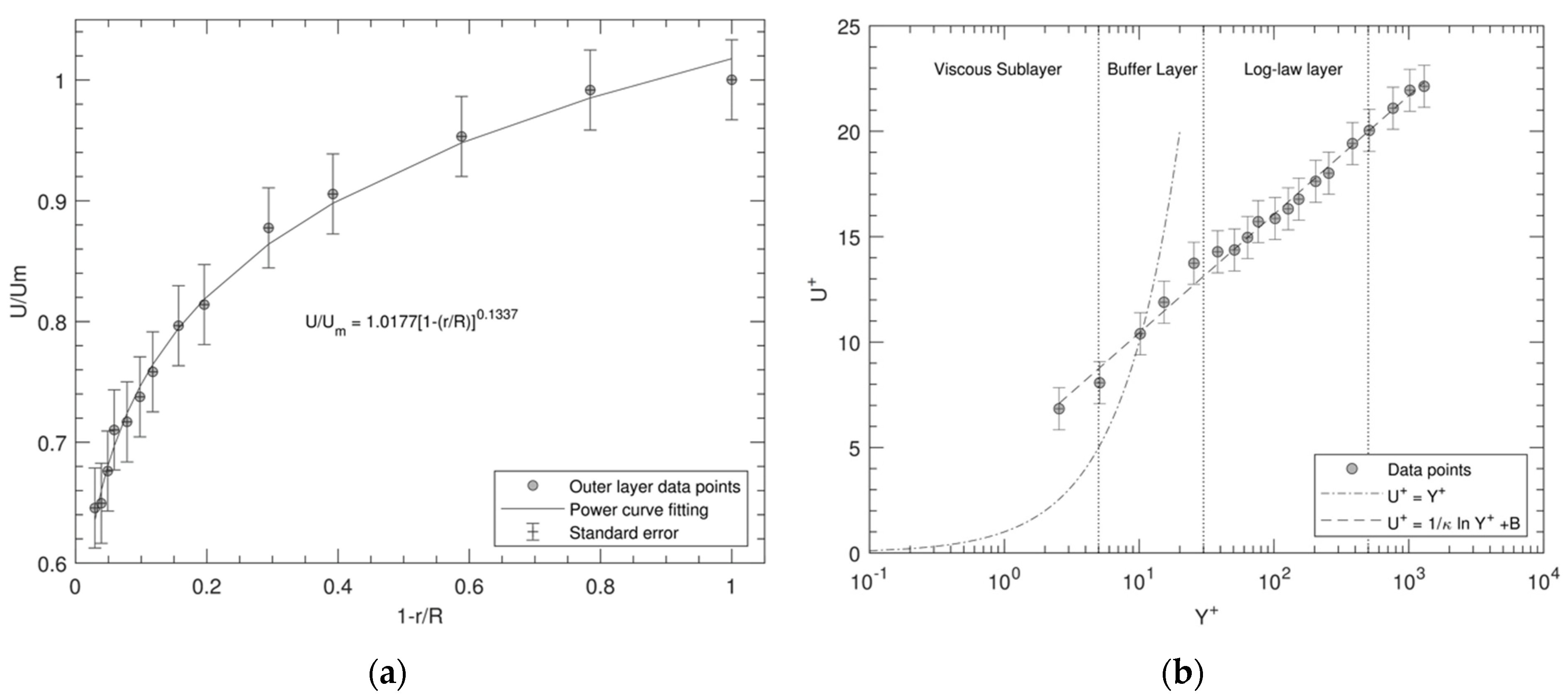
Figure 2a displays the normalized velocities over the normalized distance from the wall in linear axes. To best illustrate the velocity distribution across the pipe, the normalized velocity $\frac{U}{U_m}$ was plotted against $1-\frac{r}{R}$, with the maximum velocity naturally obtained at the centerline, $U_m=8.69\mathrm{m}/\mathrm{s}$. In this experiment, the Reynolds number was found to be very high ($Re=57,469>>4000$), validating the assumption of a turbulent regime. Figure 2a, which shows the turbulent region, excluding the viscous sub-layer and its approximation by a parameter-fitted power-law curve, illustrates that the power-law exponent n was found to be 7.48, thus deviating by approximately $7\%$ from the one-seventh power-law rule (Equation (9)). It also demonstrates that the total velocity corresponded to $\approx 68\%$ of the centerline velocity.

Figure 2b presents the three characteristic regions of the turbulent boundary layer, which can be distinguished as viscous sub-layer, buffer layer, and log-law layer. It shows that the data matched the wider theoretical representations of the turbulent flow field regions [22,29,54,55]. The flow in the viscous sublayer was very close to the tube wall and it was laminar, $0\le y^{+}\le 5$. In the buffer layer, the turbulence was progressively rising, $5\le y^{+}\le 30$, and the flow in the turbulent or log-law layer was turbulent, $y^{+}\ge 30$.

3.2. Experimental Results: Wall Shear Stress Analysis

3.2.1. Static Pressure Drop

The wall shear stress related to the pressure drop over a known length of the pipe was calculated by the pressure difference in millimeters of water. The value obtained from an analogue manometer was $2.7 {\mathrm{mmH}}_2\mathrm{O}$ for a length of $3.81 \mathrm{m}$. Using Equation (11), the wall shear stress measured by this method was found to be:

$${\tau }_w=0.182 Pa$$

3.2.2. Mean Square Signal (45° Hot-Wire)

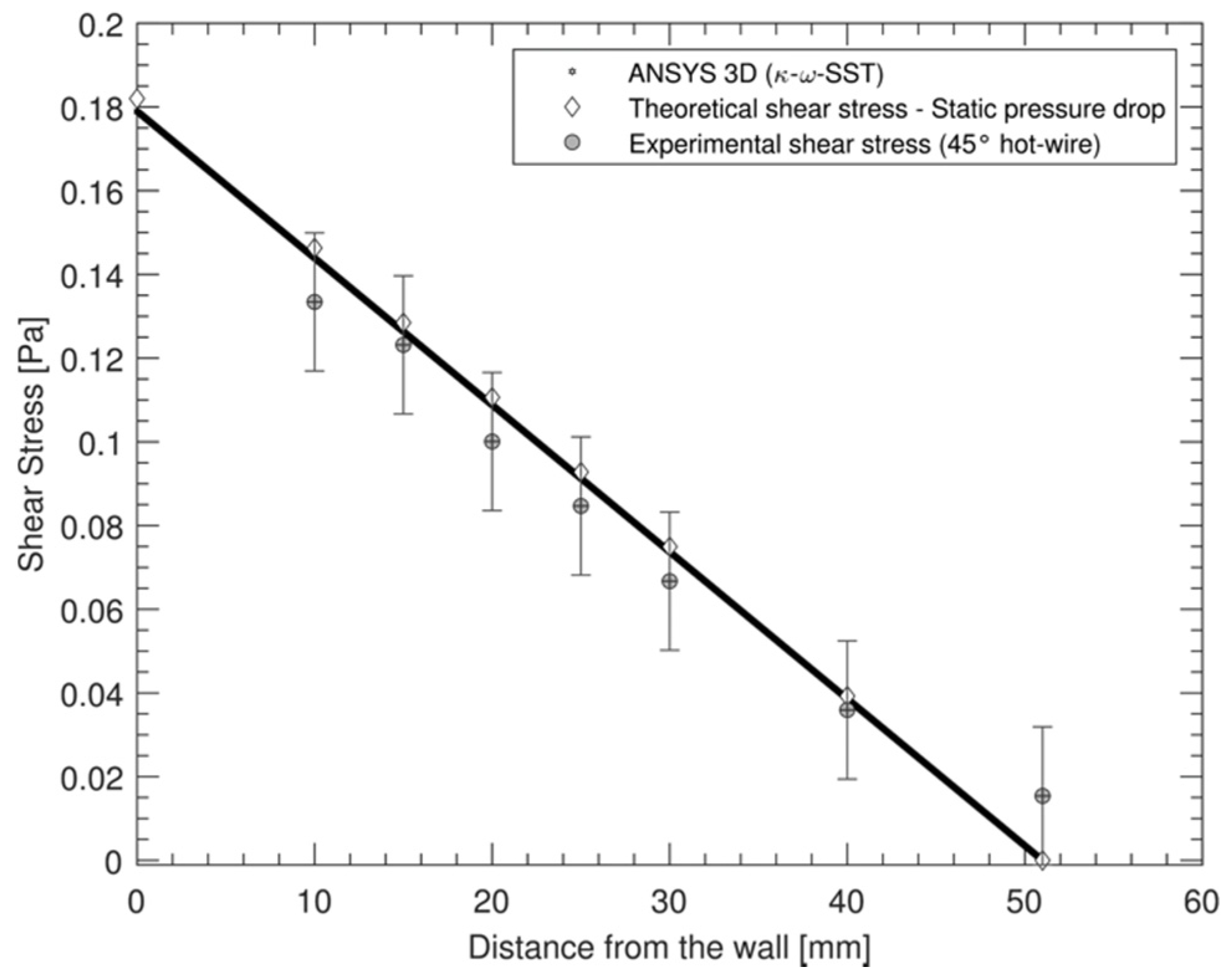
The shear stress at the wall in the mean square signal method was quantified by extrapolating the best fitted line of the experimental results. The linear best-fit equation, shown in Figure 3, was used to find the value of the wall shear stress when $r=0$. Measurements of the RMS voltage were taken at 10 mm increments along the diameter of the pipe. The Reynolds shear stresses were obtained through Equations (14) and (15) and the linear fit shear stress was computed by Equation (16). Thus, the wall shear stress using the mean square signal of a hot-wire was estimated as:

$${\tau }_w=0.162 Pa$$

3.2.3. Preston Tube

The wall shear stress was measured using a Preston tube, positioned so that its outer surface was tangential to the pipe wall while facing upstream. An appropriate configuration of the analogue manometer enabled the dynamic pressure to be read. The pressure reading was $\delta P=2.7{\mathrm{mmH}}_2\mathrm{O}$. Using Equations (18) to (21), $X^{*}=1.890$ and $Y^{*}=1.927$ were obtained. Finally, applying Equation (22) resulted in the following wall shear stress:

$${\tau }_w=0.188 Pa$$

3.2.4. Clauser Plot

Figure 4 represents the Clauser plot, illustrating that, when comparing the experimental data with the chart for experimental determination of turbulent skin friction coefficient [13], the best fit line was nearly aligned with the constant $C_f$line at 0.004. Thus, the wall shear stress was calculated from Equation (28), giving a value of:

$${\tau }_w=0.178 Pa$$

Figure 5 depicts the variation of the dimensionless velocity $U^{+}$ against the dimensionless distance $Y^{+}$, obtained from the data of the mean-square signal from a hot-wire. This graph shows that the results were in agreement with the theory of the law of the wall (see Figure 2b).

3.2.5. Error of Measurement

The margin of error in this work was reported to be within $2\%$ in the hot-wire measurements of the mean velocity fluctuations using a CTA with linearizer [34]. The pressure error was the same order as the experimental uncertainty due to the difficult nature of turbulent flow over an orifice. The errors on hot-wire positioning and velocity measurements were $25 \mathsf{\mu }\mathrm{m}$ and $0.25\mathrm{m}/\mathrm{s}$ respectively. Data points were accepted if they were 2–3 times the reference profile of the error bars; if they were beyond this value, they were considered inconsistent. The data managed a close agreement with the reference solution, the mean pressure-gradient method, and all the experimental points obtained were consistent.

3.3. Computational Results

Analysis of different aspects of turbulence modelling, mesh independency, and periodic boundary conditions helped to define the optimal parameters for the CFD simulation. The CFD simulation was validated against the data points obtained from the experiment, using the mean square signal from the hot-wire method. One of the most important aspects for analysis is the sensitivity to the grid. The sensitivity test permits the CFD user to analyze the effects of fluid behavior with the variation of a specific parameter in the simulation [56].

3.3.1. Mesh Independency

A mesh independency study was performed to examine the appropriate mesh to give an approximation of numerical error in the CFD simulation. In this study, four significantly different grid resolutions were simulated and compared, as shown in

Table 4. Comparative table of mesh independency tests.

Turbulencemodel	$k-\omega -SST$
Discretization Scheme	Second-order upwind
Convergence Criteria	1.0 × 10−6
P-V Coupling Scheme	SIMPLE Scheme
Processors in Parallel	4
Boundary Conditions	-No-slip in the walls -Periodic inlet/outlet
Grid method	3D Multiblock—Hexahedral mesh
Number of cells	3060 (coarse)	9520 (medium)	30,240 (fine)	90,045 (very fine)
Iterations to Converge	13,589	4510	12,914	26,625
Maximum Wall Y+	0.053	0.028	0.028	0.025
CPU User time	1463.88 s	764.764 s	4890.82 s	55,457.7 s
Wall clock	126.53 s	99.75 s	1016.62 s	13,339.77 s
Mbytes used cells	3	9	29	77
Virtual Memory Usage	0.258 GB	0.279 GB	0.366 GB	0.414 GB

. For validation, the results of the velocity profile were plotted in logarithmical scale (see Figure 6).

Remarkably, out of the four different types of mesh simulated (see Table 1), the medium mesh (9520 cells) gave a good resolution that only differed $1\%$ from the finest mesh and exhibited the same level of accuracy but with far lower computational times and memory usage. While it is generally assumed that significant improvements can always be attained when refining the mesh [53], the results demonstrate that this is not always necessarily the case; with 9520 cells, the result is mesh independent. It is worth noting that, despite the benefits of hexahedral cells, even this non-orthogonal cell can reduce the numerical stability of the solution and it can also produce a slower convergence [57].

3.3.2. Turbulence Models Comparison

Having established the medium mesh as the optimal mesh, two-equations turbulence models were simulated: $k-\epsilon$, $k-\omega$ and $k-\omega -SST$. Detailed information on the simulation of each model is presented in

Table 5. Comparative table of turbulence models tests.

Turbulence Model	$\mathbf{Standard}\mathit{k}-\mathit{\epsilon }$	$\mathbf{Standard}\mathit{k}-\mathit{\omega }$	$\mathit{k}-\mathit{\omega }-\mathit{S}\mathit{S}\mathit{T}$
Grid method	3D Multiblock—Hexahedral mesh
Number of cells	9520
Discretization Scheme	Second-order upwind
P-V Coupling Scheme	SIMPLE Scheme
Boundary Conditions	-No-slip in the walls-Periodic inlet/outlet
Residual Value	1.0 × 10−6
Processors in Parallel	4
Iterations	5084	4668	4510
Maximum Wall Y+	0.030	0.027	0.028
CPU User time	736.964 s	643.301 s	764.764 s
Wall clock	92.241 s	82.750 s	99.751 s
Mbytes used cells	6	6	9
Virtual Mem Usage	0.263 GB	0.263 GB	0.279 GB

.

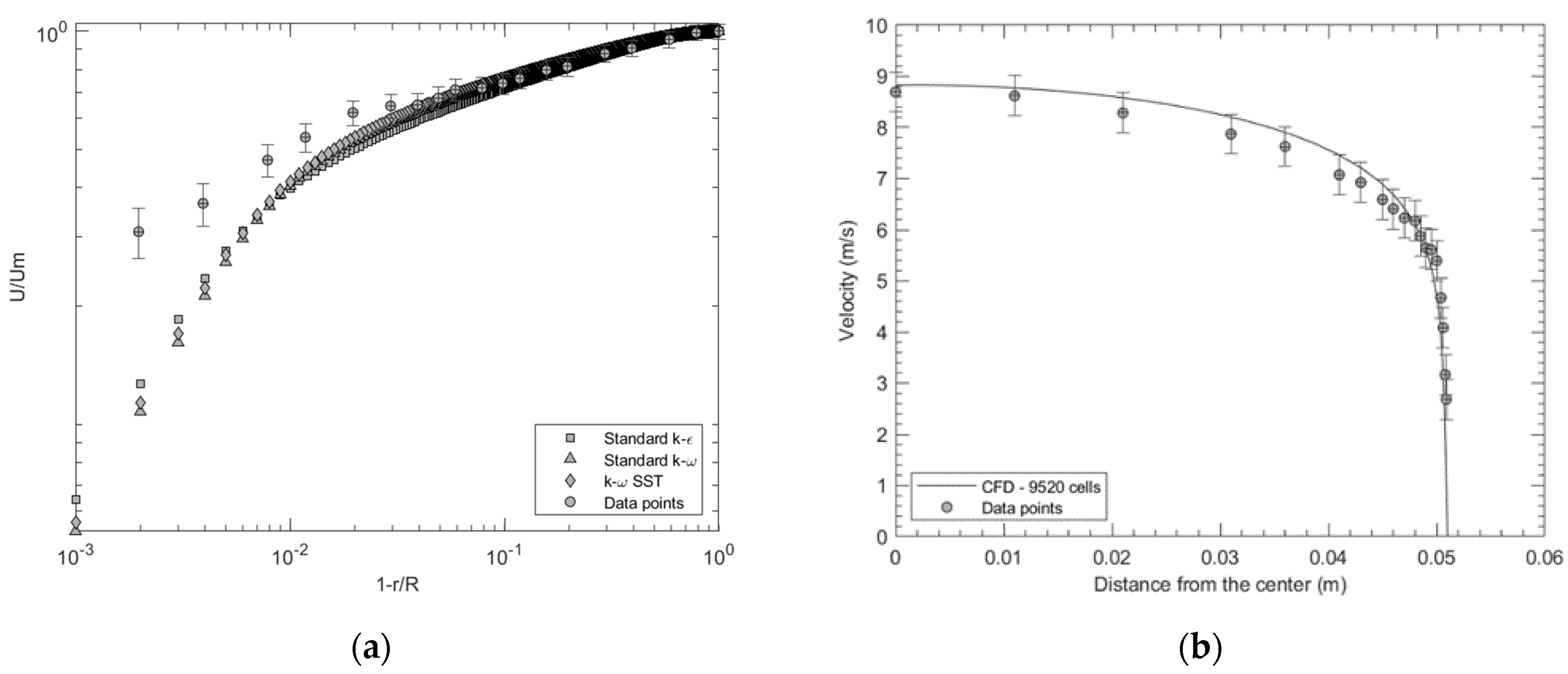
Despite its longer computational time and higher memory usage, the $\kappa -\omega -STT$ model offers results which exhibit a closer resemblance to the experimental data, as shown in Figure 7a. It is interesting to note that fewer iterations are necessary for the turbulence model $\kappa -\omega -STT$ to converge with the approximated solution.

The post-processing tool was used to generate the contour of velocity of the medium mesh with periodic boundary conditions and the $\kappa -\omega -STT$ turbulence model. Measured at the outlet of the pipe, the contour showed that the lowest velocities could be found at the pipe wall while the highest velocities could be observed at the pipe center and that the velocity progressively increased, from nearly $0\mathrm{m}/\mathrm{s}$ next to the pipe wall to $8.818 \mathrm{m}/\mathrm{s}$ for the center (see Figure 7b).

3.4. Experimental vs. Computational Results

3.4.1. Velocity Profiles Comparison

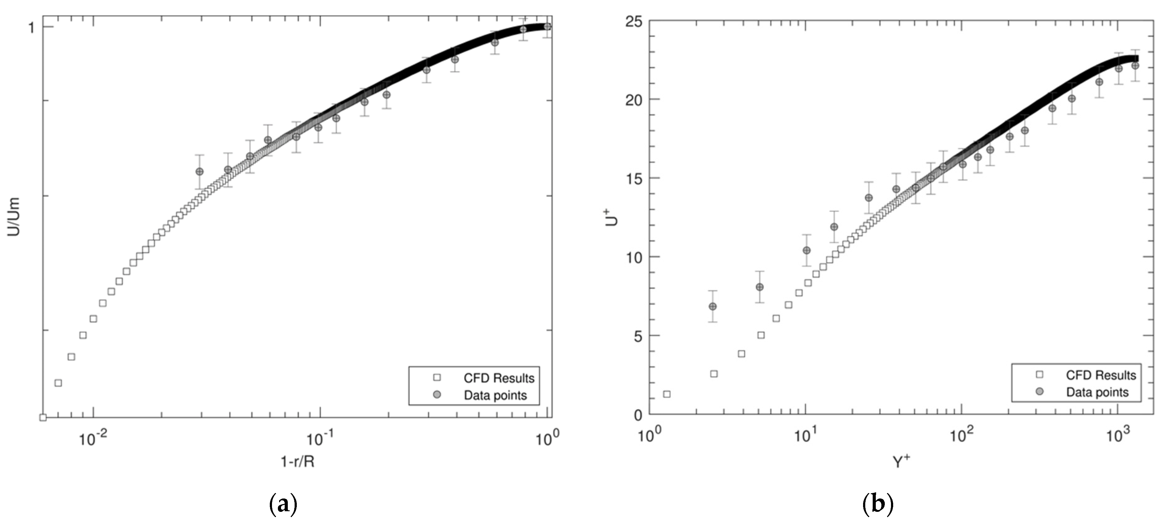
A comparison of the experimental and computational results for the velocity profiles across the pipe, presented on logarithmic axes in Figure 8a for an easier assessment of the flow near the boundaries, indicated a satisfactory agreement between the two methodologies, albeit with higher discrepancies appearing near the wall boundary. Moreover, comparing the dimensionless velocity profile across the pipe, as shown in Figure 8b, likewise denoted a good agreement between the results obtained from the experimental and computational methods, although there were some inconsistent values close to the wall due to the presence of the turbulence velocity.

3.4.2. Wall Shear Comparison

As with the velocity profile distribution, a comparison of the theoretical, experimental and computational data for the shear stress distribution across the pipe surface, as shown in Figure 9, indicated a close agreement between the results of the computational and experimental methods. The CFD simulation produced almost identical results to the theoretical results close to the wall and near to the centerline, while small differences appeared with the theoretical distribution in the region $1-\frac{r}{R} \in \left(0.61,0.10\right)$. This region coincided with the region of the pipe where the velocity field deviated most from the experimental results.

3.5. Assessment of Errors

As the only direct method, the static pressure drop method was taken as the reference point for assessing the validity of each method applied in this research for the estimation of the wall shear stresses caused by fully developed turbulent flow.

Table 6. Comparison of the experimental and computational methods for the calculation of wall shear stresses.

Method	Wall Shear Stress [Pa]	Error
Mean Pressure—Gradient method	0.182	Reference
3D CFD	0.179	+1.6%
The law of the wall	0.178	+2.2%
Preston tube	0.188	+3.3%
Mean square signal from a hot-wire	0.162	+10.4%

summarizes the findings of comparing the experimental and computational results. It illustrates that the CFD wall shear stress returned the closest agreement with the reference solution, with an error of approximately $1.6\%$compared to the experimental data. Interestingly, the CFD results were positioned exactly between the theoretical and experimental results of the mean square signal from a hot-wire method.

4. Conclusions

The results of this research show that axisymmetric RANS simulations can potentially produce a close agreement with experimental methods for studying fluid turbulence and comparing the velocity profile and wall shear stress of turbulent flow in a pipe. This finding demonstrates that, while the RANS method certainly does not capture all the flow physics shown in the laboratory measurements and while commercial packages such as ANSYS Fluent require significant computing power and time for calculation in order to obtain results with a minimum error, CFD can still be used as an alternative or addition to experimental methods for analyzing a fully developed turbulent pipe flow, at least after it has been validated against experimental techniques. This indicates the advances made in the evolution of methods used for studying fluid turbulence over the last 100 years and the development of cost-effective computational methods that do not require the infrastructure for the experimental methods.

References

1. Çengel, Y.; Turner, R.; Cimbala, J. Fundamentals of Thermal-Fluid Sciences, 3rd ed.; McGraw Hill: New York, NY, USA, 2008. [Google Scholar]
2. Perry, A. Hot-Wire Anemometry; Oxford University Press: Oxford, UK, 1982. [Google Scholar]
3. Vardy, A.; Brown, J. Transient Turbulent Friction in Smooth Pipe Flows. J. Sound Vib. 2003, 259, 1011–1036. [Google Scholar] [CrossRef]
4. Reynolds, O. An Experimental Investigation of the Circumstances Which Determine Whether the Motion of Water Shall Be Direct or Sinuous, and of the Law of Resistance in Parallel Channels. Philos. Trans. R. Soc. 1883, 174, 935–982. [Google Scholar] [CrossRef] [Green Version]
5. Turns, S. Thermal-Fluid Sciences; Cambridge University Press: Cambridge, UK, 2006. [Google Scholar]
6. Boussinesq, M. Calcul Du Pouvoir Refroidissant des Courants Fluids. J. Math Pures Appl. 1905, 6, 285–332. [Google Scholar]
7. Russel, A. The Convection of Heat from a Body Cooled by a Stream of Fluid. Lond. Edinb. Dublin Philos. Mag. J. Sci. 1911, 20, 591–610. [Google Scholar] [CrossRef]
8. King, L. On the Convection of Heat from Small Cylinders in a Stream of Fluid: Determination of the Convection Constants of Small Platinum Wires with Applications to Hot-Wire Anemometry. Proc. R. Soc. A Math. Phys. Eng. Sci. 1914, 90, 373–432. [Google Scholar] [CrossRef] [Green Version]
9. Dryden, H.; Kuethe, A. The Measurement of Fluctuations of Air Speed by the Hot-Wire Anemometer. Available online: https://ntrs.nasa.gov/search.jsp?R=19930091390 (accessed on 13 August 2018).
10. Gad-el-Hak, M. Advances in Fluid Mechanics Measurements; Springer: Berlin/Heidelberg, Germany, 1989. [Google Scholar]
11. Head, M.; Rechenberg, I. The Preston Tube as a Means of Measuring Skin Friction. J. Fluid Mech. 2006, 14, 1–17. [Google Scholar] [CrossRef]
12. Preston, J. The Determination of Turbulent, Skin Friction by Means of Pitot Tubes. J. R. Aeronaut. Soc. 1954, 58, 109–121. [Google Scholar] [CrossRef]
13. Clauser, F. The Turbulent Boundary Layer. Adv. Appl. Mech. 1956, 4, 1–51. [Google Scholar] [CrossRef]
14. Fernholz, H.; Finley, P. The Incompressible Zero-Pressure-Gradient Turbulent Boundary Layer: An Assessment of the Data. Prog. Aerosp. Sci. 1996, 32, 245–311. [Google Scholar] [CrossRef]
15. Versteeg, H.; Malalasekera, W. An Introduction to Computational Fluid Dynamics; Pearson: London, UK, 1995. [Google Scholar]
16. Kapelson, A. Computational of Mean Velocity Distribution in a Turbulent Flow. Available online: https://arxiv.org/abs/physics/9904030 (accessed on 12 November 2017).
17. Deardorff, J. A Numerical Study of Three-Dimensional Turbulent Channel Flow at Large Reynolds Numbers. J. Fluid Mech. 1970, 41, 453–480. [Google Scholar] [CrossRef]
18. Menter, F. Two-Equations Eddy-Viscosity Turbulence Models for Engineering Applications. AIAA J. 1994, 32, 1598–1605. [Google Scholar] [CrossRef] [Green Version]
19. Smagorinsky, J. General Circulation Experiments with the Primitive Equations. Mon. Weather Rev. 1963, 91, 99–164. [Google Scholar] [CrossRef]
20. Orszag, S.; Patterson, G. Numerical Simulation of Turbulence: Statistical Models and Turbulence; Springer: Berlin/Heidelberg, Germany, 1972. [Google Scholar]
21. Craft, T. Finite Difference Schemes, CFD Mechanical Aerospace and Civil Engineering Manchester Website. Available online: http://cfd.mace.manchester.ac.uk/twiki/pub/Main/TimCraftNotes_All_Access/cfd1-findiffs.pdf (accessed on 16 July 2018).
22. Launder, B.; Spalding, D. Mathematical Models of Turbulence; Academic Press: London, UK, 1972. [Google Scholar]
23. Keshmiri, A. Numerical Sensitivity Analysis of 3- and 2-Dimensional Rib-Roughened Channels. Heat Mass Transf. 2012, 48, 1257–1271. [Google Scholar] [CrossRef]
24. Keshmiri, A.; Cotton, M.; Addad, Y.; Rolfo, S.; Billard, F. RANS and LES Investigations of Vertical Flows in the Fuel Passages of Gas-Cooled Nuclear Reactors. In Proceedings of the 16th International Conference on Nuclear Engineering, Orlando, FL, USA, 11–15 May 2008; Volume 2, pp. 297–306. [Google Scholar] [CrossRef] [Green Version]
25. Keshmiri, A.; Cotton, M.; Addad, Y.; Laurence, D. Turbulence Models and Large Eddy Simulations Applied to Ascending Mixed Convection Flows. Flow Turbul. Combust. 2012, 89, 407–434. [Google Scholar] [CrossRef]
26. Keshmiri, A.; Osman, K.; Benhamadouche, S.; Shokri, N. Assessment of Advanced RANS Models against Large Eddy Simulation and Experimental Data in the Investigation of Ribbed Passages with Passive Heat Transfer. Numer. Heat Transf. Part B Fundam. 2016, 69, 96–110. [Google Scholar] [CrossRef] [Green Version]
27. Keshmiri, A.; Revell, A.; Darabkhani, H. Assessment of a Common Nonlinear Eddy-Viscosity Turbulence Model in Capturing Laminarization in Mixed Convection Flows. Numer. Heat Transf. Part A Appl. 2016, 69, 146–165. [Google Scholar] [CrossRef] [Green Version]
28. Keshmiri, A.; Uribe, J.; Shokri, N. Benchmarking of Three Different CFD Codes in Simulating Natural, Forced and Mixed Convection Flows. Numer. Heat Transf. Part A Appl. 2015, 67, 1324–1351. [Google Scholar] [CrossRef]
29. Pope, S. Turbulent Flows, 7th ed.; Cambridge University Press: Cambridge, UK, 2001. [Google Scholar]
30. Hurst, D.; Vassilicos, J. Scaling and Decay of Fractal-Generated Turbulence. Phys. Fluids 2007, 19, 035103. [Google Scholar] [CrossRef] [Green Version]
31. Chamorro, L.; Porte-Agel, F. A Wind-Tunnel Investigation of Wind-Turbine Wakes: Boundary-Layer Turbulence Effects. Bound. -Layer Meteorol. 2009, 132, 129–149. [Google Scholar] [CrossRef] [Green Version]
32. Lomas, C. Fundamentals of Hot Wire Anemometry; Cambridge University Press: Cambridge, UK, 1986. [Google Scholar]
33. Bruun, H.H. Hot-Wire Anemometry: Principles and Signal Analysis; Oxford University Press: Oxford, UK, 1995. [Google Scholar]
34. Comte-Bellot, G. Hot-Wire Anemometry. Annu. Rev. Fluid Mech. 1976, 8, 209–231. [Google Scholar] [CrossRef]
35. Neu, M. Hot-Wire and Hot-Film Anemometry. Available online: http://www.dept.aoe.vt.edu/~simpson/aoe4154/hotwirelab.pdf (accessed on 23 March 2021).
36. McDonough, J. Introductory Lectures on Turbulence: Physics, Mathematics and Modeling. Available online: https://uknowledge.uky.edu/me_textbooks/2 (accessed on 23 March 2021).
37. Harotinidis, J.H. The Measurement of Wall Shear Stress. Adv. Fluid Mech. Meas. 1989, 45, 229–261. [Google Scholar] [CrossRef]
38. Tropea, C.; Yarin, A.; Foss, J. Springer Handbook of Experimental Fluid Mechanics; Springer: Chicago, IL, USA, 2007. [Google Scholar]
39. Patel, V. Calibration of the Preston Tube and Limitations on Its Use in Pressure Gradients. J. Fluid Mech. 1965, 23, 185–208. [Google Scholar] [CrossRef]
40. Wei, T.; Schmidt, R.; McMurtry, P. Comment on the Clauser Chart Method for Determining the Friction Velocity. Exp. Fluids 2005, 38, 695–699. [Google Scholar] [CrossRef]
41. Sherman, F. Viscous Flow; McGraw-Hill: New York, NY, USA, 1990. [Google Scholar]
42. Eggels, J.; Unger, F.; Weiss, M.; Westerweel, J.; Adrian, R.; Friedrich, R.; Nieuwstadt, F. Fully Developed Turbulent Pipe Flow: A Comparison between Direct Numerical Simulation and Experiment. J. Fluid Mech. 1994, 268, 175–209. [Google Scholar] [CrossRef]
43. Evola, G.; Popov, V. Computational Analysis of Wind Driven Natural Ventilation in Buildings. Energy Build. 2006, 5, 491–501. [Google Scholar] [CrossRef]
44. Khier, W.; Breuer, M.; Durst, F. Flow Structure around Trains under Side Wind Conditions: A Numerical Study. Comput. Fluids 2000, 29, 179–195. [Google Scholar] [CrossRef]
45. Kleinstreuer, C.; Zhang, Z. Laminar-to-Turbulent Fluid-Particle Flows in a Human Airway Model. Int. J. Multiph. Flow 2003, 2, 271–289. [Google Scholar] [CrossRef]
46. Umlauf, L.; Burchard, H.; Hunter, K. Extending the K-w Turbulence Model towards Oceanic Applications. Ocean Model. 2003, 3, 195–218. [Google Scholar] [CrossRef]
47. Wilcox, D. Turbulence Modeling for CFD, 2nd ed.; DCW Industries: La Canada Flintridge, CA, USA, 1998. [Google Scholar]
48. Menter, F. Zonal Two Equation K-ω Turbulence Models for Aerodynamic Flows. In Proceedings of the 23rd Fluid Dynamics, Plasmadynamics, and Lasers Conference, Orlando, FL, USA, 6–9 July 1993; Volume 32, pp. 1598–1605. [Google Scholar] [CrossRef]
49. ANSYS 7.3.16. Periodic Boundary Conditions. Available online: www.afs.enea.it/project/neptunius/docs/fluent/html/ug/node252 (accessed on 29 January 2018).
50. Craft, T. Turbulence and Related Modelling, CFD Mechanical Aerospace and Civil Engineering Manchester Website. Available online: http://cfd.mace.manchester.ac.uk/twiki/pub/Main/TimCraftNotes_All_Access/ms4-turbflow.pdf (accessed on 16 July 2018).
51. Patankar, S. Numerical Heat Transfer and Fluid Flow; Taylor & Francis: New York, NY, USA, 1980. [Google Scholar]
52. Keshmiri, A.; Gotts, J. Thermalhydraulic Analysis of Four Geometrical Design Parameters in Rib-Roughened Channels. Numer. Heat Transf. Part A Appl. 2011, 60, 305–327. [Google Scholar] [CrossRef]
53. Keshmiri, A. Three-dimensional simulation of a simplified advanced gas-cooled reactor fuel element. Nucl. Eng. Des. 2011, 241, 4122–4135. [Google Scholar] [CrossRef]
54. Laufer, J. The Structure of Turbulence in Fully Developed Pipe Flow. Available online: https://ntrs.nasa.gov/archive/nasa/casi.ntrs.nasa.gov/19930083975.pdf (accessed on 13 August 2018).
55. Keshmiri, A.; Addad, Y.; Cotton, M.A.; Laurence, D.R.; Billar, F.; Billard, F. Refined eddy viscosity schemes and large eddy simulations for ascending mixed convection flows. In Proceedings of the 4th International Symposium on Advances in Computational Heat Transfer, “CHT08”, Marrakech, Morocco, 11–16 May 2008; Paper CHT-08-407. Volume 44, pp. 1–22. [Google Scholar]
56. Keshmiri, A. Effects of Various Physical and Numerical Parameters on Heat Transfer in Vertical Passages at Relatively Low Heat Loading. J. Heat Transf. 2011, 133, 092502. [Google Scholar] [CrossRef] [Green Version]
57. Casey, M.; Wintergerste, T. European Research Community on Flow, Turbulence and Combustion] Special Interest Group on “Quality and Trust in Industrial CFD” Best Practice Guidelines; ERCOFTAC: London, UK, 2000. [Google Scholar]
Figure 1. Test rig for the study of fully developed turbulent flow in a pipe: (a) Equipment at the pipe exit; (b) Digital devices used in this experiment.
Fluids 07 00078 g001
Figure 2. (a) Approximation of the normalized velocity fitted with the power-law curve; (b) Dimensionless velocity profile showing the regions of the turbulent boundary layer.
Fluids 07 00078 g002
Figure 3. Theoretical and experimental shear stress across the pipe.
Fluids 07 00078 g003
Figure 4. Semi-logarithmic plot with the best fit line of C f .
Fluids 07 00078 g004
Figure 5. Dimensionless velocity over dimensionless distance from the wall.
Fluids 07 00078 g005
Figure 6. Comparison of the normalized velocity profile for different mesh resolution plotted in log-log scale.
Fluids 07 00078 g006
Figure 7. (a) Comparison of the normalized velocity profile for different turbulence models; (b) Velocity profile.
Fluids 07 00078 g007
Figure 8. Velocity profiles comparison between experimental and CFD results: (a) Normalized velocity versus the dimensionless distance from the pipe wall on logarithmic axes; (b) Dimensionless velocity U+ versus the dimensionless distance from the pipe wall Y+.
Fluids 07 00078 g008
Figure 9. Comparison of experimental, theoretical and CFD results of the shear stress distribution across the pipe.
Fluids 07 00078 g009