Numerical Simulation of Departure from Nucleate Boiling in Rod Bundles under High-Pressure Conditions

Abstract

In subcooled boiling flows beyond a certain heat flux, heat transfer is hampered due to a phenomenon known as Departure from Nucleate Boiling (DNB). Conducting DNB experiments at one-to-one nuclear reactor operating conditions is highly challenging and expensive. Another alternative approach is to use Look-up table data. However, its applicability is limited due to its dependence on rod bundle correction factors. In the present investigation, a state-of-the-art Eulerian-Eulerian two-fluid model coupled with an extended heat flux partitioning model is used to predict DNB in tubes and rod bundles with square and hexagonal lattices (relevant to Pressurized Water Reactors). In this approach, bubble departure characteristics are modeled using semi-mechanistic models based on force balance analysis. The predicted DNB values are compared with experimental and Look-up table data and found out to be within 1.8% to 20%.

1. Introduction

Flow boiling is widely used in many industries as a heat transfer mechanism due to its excellent heat transfer characteristics. Some degree of boiling may happen in all water-cooled nuclear reactors depending on the operational states, irrespective of the type of reactors. In the reactor core of Pressurized Water Reactors (PWRs), subcooled boiling may occur. Heat transfer characteristics of boiling flows are better than single-phase flows. However, the heat transfer rate decreases drastically beyond a specific heat flux, and this limiting heat flux is referred to as Critical Heat Flux (CHF), and it depends on operating conditions. At subcooled and near saturation conditions, increased vapor bubble generation near the heater surface can prevent the liquid from wetting the heating surface. This phenomenon is called Departure from Nucleate Boiling (DNB). Since DNB occurs at very high heat fluxes, it has more detrimental effects on the fuel pin temperatures in PWRs. The ratio between DNB and the actual operating local heat flux is called the departure from nucleate boiling ratio (DNBR), which may change axially and radially in the reactor. The minimum value of DNBR, which is known as MDNBR, defines thermal margins [1]. According to some regulatory bodies, the typical MDNBR should be at least 1.3. In view of the above, it is paramount to determine DNB to evaluate the thermal design margins of these reactors.

DNB primary depends on the physics of boiling flows, which is extremely complex as it involves intricate microscopic processes like bubble nucleation, growth, departure, coalescence, and breakage. Hence, determining DNB from the first principles has always been a great challenge to the researchers. So, over the years, dozens of dedicated experiments have been conducted worldwide to determine DNB for various geometries and operating conditions [2], even a few on PWR-specific rod bundles [3]. DNB experiments are usually performed in scaled facilities to minimize the power requirement. Decades of experimentation have yielded empirical correlations with limited validity for the range of geometry and test conditions [4]. It is important to note that conducting experiments at high pressure and high temperature (HPHT) conditions, especially for PWR rod bundles, is technically challenging and highly expensive. Another approach for DNB evaluation is to use Look-up tables [5,6], which are developed based on large sets of experimental data. However, even the usage of Look-up table data is limited due to their dependency on rod bundle correction factors which are to be obtained through experiments. In the last few decades, the increase in computational power has encouraged researchers to investigate DNB using computational fluid dynamics (CFD) techniques.

Over the years, the Eulerian-Eulerian two-fluid model coupled with the heat flux partitioning model (EEHFP) has been used to study the characteristics of boiling flows [7,8,9,10]. Generally, in the heat flux partitioning (HFP) model, the heat flux is partitioned into three components, heat flux for vapor generation, quenching (In a bubble ebullition cycle, cold liquid replaces the bubble as the bubble lifts-off of the surface. The heat is assumed to be transferred to the cold liquid due to transient conduction. This process is referred to as quenching) and liquid convection. In recent years, researchers extended the HFP model by considering other phenomena like bubble sliding [11] and heat transfer to vapor [12,13]. The HFP models, where heat transfer to vapor is considered only after reaching a preset condition based on the vapor fraction, are widely used to predict DNB in tubes and rod bundles. A summary of a few important studies on DNB prediction based on the EEHFP model is discussed below.

Zhang et al. [14] used Ioilev et al. [15] partitioning model to predict DNB in tubes. Li et al. [16] predicted DNB in vertical tubes using an extending wall boiling model based on the near-wall cell’s void fraction. They used Look-up table [5] data for validation and found the maximum deviation to be 20% for uniform heat flux profiles. They have also reported the influence of critical void fraction on DNB’s prediction and suggested that it varies with pressure and mass flux. Kim et al. [17] predicted DNB in 11 configurations with non-mixing vane grids (NMVGs) and seven tests with mixing vane grids (MVGs) and found that the error as compared to experimental data was less than 16% for NVMGs, and the maximum error was 26% for MVGs. Moreover, they reported that the error increased by up to 45% at high subcooling test conditions. They calculated critical void fraction based on void fraction at a specified wall y+ (~200). Improving upon their previous study, Kim et al. [18] considered lift and wall lubrication forces (Lift force is due to liquid shear, and the wall lubrication force is a hydrodynamic force resulting from the presence of liquid between the bubble and wall.) via Sugrue et al. [19] and Lubchenko et al. [20] models, respectively. They investigated 15 tubular cases of Thompson and Macbeth [21], for which they found the error to be within 25%. They have found that the deviation of predicted DNB from the experimental data increased with an increase in subcooling and suggested that it could be due to the quenching closures (bubble wait time and area influence coefficient). Xu et al. [22] predicted DNB in rod bundles with mixing vanes under PWR conditions; however, their study was restricted to the mass flux of about 3600 kg/m²s. They reported that the lift force has a significant impact on radial void fraction and temperature distributions. Zhang et al. [23] performed CFD analysis to predict CHF in a 2 × 2-rod bundle; however, the subcooled region was not covered in their study. They used a similar model to Zhang et al. [14]. Vadlamudi and Nayak [24] predicted DNB in vertical tubes. They reported that the predictions were within 15%. Notably, when the outlet quality was more than or equal to −0.10, the predictions were within 6% compared with experimental data [21].

In all these previous numerical works based on the EEHFP model for DNB prediction, as discussed above, empirical models were used to determine bubble departure characteristics. Bubble departure dynamics play a vital role in heat flux partitioning. The applicability of the EEHFP model is limited due to reliance on empirical correlations for such departure characteristics. Moreover, improper selection of non-physical models might lead to unrealistic results [24]. Incorporating more physical models will improve the confidence in the EEHFP model for simulating such complex phenomena (like DNB).

In the present work, the EEHFP model has been used with semi-mechanistic formulations based on force balance analysis for bubble departure diameter and departure frequency to predict DNB in rod bundles with square lattice and hexagonal lattice relevant to PWRs. The model has been validated with tubular experimental data [21] and the rod bundle experimental data [25]. The hexagonal lattice DNB predictions have been compared with Look-up tables with appropriate corrections.

2. Mathematical Model

In the EEHFP framework, both phases are solved in the Eulerian framework. The details pertaining to governing equations of continuity, momentum, and energy were discussed in detail in many previous publications [8,26]. In this paper, the emphasis is given to the heat flux partitioning model and boiling closures.

2.1. Heat Flux Partitioning Model

The applied wall heat flux is partitioned into four components, liquid phase convective flux (${q^{″}}_c$), evaporative flux (${q^{″}}_e$), quenching flux (${q^{″}}_q$), and vapor phase convective flux (${q^{″}}_v$).

$${q^{″}}_{total}=\left({q^{″}}_c+{q^{″}}_q+{q^{″}}_e\right)f\left(\alpha \right)+\left(1-f\left(\alpha \right)\right)\left({q^{″}}_v\right)$$

(1)

$${q^{″}}_c=h_c\left(T_w-T_l\right)\left(1-A\right)$$

(2)

$${q^{″}}_q=\frac{2k_l}{\sqrt{\pi {\lambda }_l{t}_w}}\left(T_w-T_l\right)A$$

(3)

$${q^{″}}_e=V_b{N}_w{\rho }_v{h}_{fg}f$$

(4)

$${q^{″}}_v=h_v\left(T_w-T_v\right)A$$

(5)

where h_c and h_v are heat transfer coefficients for liquid and vapor, respectively. A is the fraction of heat surface area influenced by the evaporation process (“A” value depends on nucleation site density (N_w), bubble departure diameter (D_b), and area influence factor (k_a)). T_w, T_l and T_v are the temperatures of the wall (heater surface), liquid and vapor, respectively. k_l and λ_l are the liquid’s thermal conductivity and diffusivity, t_w is the waiting period before the next bubble’s nucleation.

Researchers [12,13,15,17] proposed different values for $f\left(\alpha \right)$. In this study, the value proposed by [15] has been chosen, and the equation goes as follows:

$$f\left(\alpha \right)=max\left(0,min\left(\frac{{\alpha }_v-{\alpha }_{v,1}}{{\alpha }_{v,2}-{\alpha }_{v,1}}\right)\right)$$

(6)

where, ${\alpha }_{v,1}=0.9$ and ${\alpha }_{v,2}=0.95$

2.2. Boiling Closures

The three most essential boiling closures are bubble departure diameter, departure frequency, and nucleation site density. It is imperative to use appropriate models for boiling closures as they, in turn, affect the vapor generation at the wall. A brief overview of the boiling closures is provided in this section.

2.2.1. Bubble Departure Diameter and Frequency

Bubble departure diameter, especially in flow boiling conditions, relies on various parameters like contact angles (advancing and receding contact angles), the liquid’s velocity, void fraction, thermodynamic properties of the liquid, wall superheats, and many others [27]. Many empirical models are widely used to determine bubble departure diameter and departure frequency. In CFD simulations, the most widely used correlation for bubble departure diameter is the model developed by Tolubinsky and Kostanchuk [28]. They gave a correlation for bubble departure diameter based on liquid subcooling. However, there is no physical basis for applying such models to high-pressure conditions. Recently, Krepper and Rzehak [7] modified the reference diameter and reference temperature of the Tolubinsky and Kostanchuk model in their study based on the experimental results.

Similarly, Vadlamudi and Nayak [24] modified the reference diameter and temperature based on Semeria (1963) experimental data for high-pressure conditions. However, the extendability of the models developed based on very few experimental points is limited. This mandates a need for better modeling techniques. Another approach that has gained a great deal of attention in the past few decades is the usage of semi-mechanistic models. Semi-mechanistic models are generally based on force balance analysis.

Important work on force balance models in flow boiling was done by Klausner et al. [27]. In recent years, researchers modified the few force formulations [29,30,31]; however, the overall framework of Klausner was retained.

The fundamental principle of force balance analysis is based on the evaluation of forces acting on the bubble. Figure 1 shows the vital forces acting on the bubble in both the flow (x) and perpendicular (y) (to wall) directions, as shown in Figure 1.

In the flow direction, essential forces to be considered are the quasi-static drag force (F_qs), x-component of surface tension force (F_stx), buoyancy force (F_b), and x-component of unsteady drag force (F_dux) (this force is due to bubble growth on the heater surface). And in the direction perpendicular to the heater surface, vital forces are shear lift force (F_sl), contact pressure force (F_cp), hydrodynamic pressure force (F_h), y-component of unsteady drag force (F_duy), and y-component of surface tension force (F_sty).

Before the departure of the bubble, during its growth phase, the surface tension force, unsteady drag force, and hydrodynamic pressure force prevent the bubble from sliding or lifting off the heater surface. At the same time, the lift force, quasi-static drag force, buoyancy force, and contact pressure force help the bubble to depart from its nucleation point. The resultant of forces in x and y directions are as follows:

$${\displaystyle \sum }{F}_x=F_{qs}+F_b-F_{dux}-F_{stx}$$

(7)

$${\displaystyle \sum }{F}_y=F_{sl}+F_{cp}-F_h-F_{sty}-F_{duy}$$

(8)

If the summation of forces is positive in either direction, then the bubble departs from its nucleation point; otherwise, it continues to grow. The formulations for all the forces are tabulated in

Table 1. Summary of forces for determining bubble departure diameters and frequencies.

x-Direction	y-Direction
Quasi-static drag force: $F_{qs}=6\pi {\rho }_l\vartheta v_{r}R\left(\frac{2}{3}+{\left[{\left(\frac{12}{Re}\right)}^n+{0.796}^n\right]}^{-1/n}\right)$ where, n = 0.65	Shear lift force: $F_{sl}=\frac{1}{2}{\rho }_l{v_r}^2\pi r^2\left(3.877{G_s}^{1/2}\times {\left[R{e}_b^{-2}+{\left(0.344{G_s}^{1/2}\right)}^4\right]}^{1/4}\right)$ $\mathrm{where}, G_s=\left|\frac{dv}{dy}\right|\frac{r}{v_r}$
Buoyancy force: $F_b=\frac{4}{3}\pi R^3\left[{\rho }_l-{\rho }_v\right]g$	Hydrodynamic pressure force: $F_h=\frac{9}{8}{\rho }_l{v_r}^2\pi \frac{d_w^2}{4}$
Unsteady drag force: $F_{dux}={\rho }_l\pi R^2\left(R\ddot{R}+\frac{3}{2}{\dot{R}}^2\right)\sin \phi$ $\phi =\pi /18$	Unsteady drag force: $F_{duy}={\rho }_l\pi R^2\left(R\ddot{R}+\frac{3}{2}{\dot{R}}^2\right)\cos \phi$ $\phi =\pi /18$
Surface tension force: $F_{stx}=1.25d_w\sigma \frac{\pi \left({\theta }_{\alpha }-{\theta }_{\beta }\right)}{{\pi }^2-{\left({\theta }_{\alpha }-{\theta }_{\beta }\right)}^2}\left(\sin {\theta }_{\alpha }+\sin {\theta }_{\beta }\right)$	Surface tension force: $F_{sty}=d_w\sigma \frac{\pi }{{\theta }_{\alpha }-{\theta }_{\beta }}\left(\cos {\theta }_{\beta }-\cos {\theta }_{\alpha }\right)$
	Contact pressure force: $F_{cp}=\pi \frac{d_w^2}{4}\frac{2\sigma }{5R}$
Contact diameter	Radius
$d_w=k_{dw}{D}_b$	$R\left(t\right)=\frac{2b}{\sqrt{\pi }}Ja\sqrt{\eta t}$

. The bubble diameter has been determined using the growth rate equation, and the diameter at the point of departure has been considered as the bubble departure diameter. From the bubble departure time, the departure frequency has been determined while considering that bubble-waiting time to be 80% of the total nucleation cycle [32].

It is important to use an appropriate bubble growth rate model to calculate bubble departure diameter and departure frequency. Usually, the bubble growth phase is broadly classified into two stages: (i) inertial controlled growth and (ii) heat-diffusion controlled growth [33]. At high pressures, low superheats, and low thermal conductivities, the growth of the bubble is majorly driven by heat diffusion [34]. For heat-diffusion controlled growth, $R\propto t^{1/2}$, where R is the bubble radius and t is the time, bubble growth rate usually takes the following form [34]:

$$R\left(t\right)=2C_1\sqrt{{\lambda }_{l}t}$$

(9)

where, ${\lambda }_l$ is thermal diffusivity of liquid, C₁ is an implicit function of Jakob number and density ratio ($\frac{{\rho }_l}{{\rho }_g}$).

Over the years, many bubble growth rate models have been proposed, and some of the most widely used models are tabulated in

Table 2. Summary of popular models used for bubble growth.

Model	Radius
Forster and Zuber [36]	$R\left(t\right)=\frac{2}{\sqrt{\pi }}Ja\sqrt{{\lambda }_{l}t}$
Plesset and Zwick [40]	$R\left(t\right)=2\left(\sqrt{\frac{3}{\pi }}\right)k_l\left(T_l-T_{sat}\right)\sqrt{{\lambda }_{l}t}$
Cooper [37]	$R\left(t\right)=\frac{2}{C_2}P{r}^{-0.5}Ja\sqrt{{\lambda }_{l}t}$
Mikic et al. [35]	$R\left(t\right)=\frac{2}{3}\frac{B^2}{A}\left[{\left(t^{+}+1\right)}^{\frac{3}{2}}-{\left(t^{+}\right)}^{\frac{3}{2}}-1\right],$ $\mathrm{where}, t^{+}=\frac{A^2}{B^2}t$ $A={\left(\frac{\pi }{7}\frac{h_{fg}{\rho }_v\Delta T_{sat}}{{\rho }_l{T}_{sat}}\right)}^{\frac{1}{2}}$ $B={\left(\frac{12}{\pi }{\lambda }_l\right)}^{1/2}\frac{\Delta T_{sat}{c}_{pl}{\rho }_l}{h_{fg}{\rho }_v}$
Yun et al. [29]	$R\left(t\right)=\frac{2b}{\sqrt{\pi }}Ja\sqrt{{\lambda }_{l}t}-\frac{b{q}^{″}}{2h_{fg}{\rho }_v}t$ $\mathrm{where}, q^{″}=h_c\left(T_{sat}-T_{sub}\right)$ and b = 1.56
Colombo and Fairweather [31]	$R\left(t\right)=\frac{2}{C_2}P{r}^{-0.5}Ja\sqrt{{\lambda }_{l}t}+2\left(\sqrt{\frac{3}{\pi }}\right)k_l\left(T_l-T_{sat}\right)\sqrt{{\lambda }_{l}t}-\frac{b{q}^{″}}{h_{fg}{\rho }_v}t$
Sugrue and Buongiorno [30]	$R\left(t\right)=\frac{2b}{\sqrt{\pi }}Ja\sqrt{{\lambda }_{l}t}$ b = 1.56

. Mikic et al. [35] model was used by Klausner [27] for the evaluation of bubble growth. The effect of condensation was incorporated by Yun et al. [29]. Sugrue and Buongiorno reported better predictions without condensation term, similar to Zuber’s original model [36]. Colombo and Fairweather [31] have developed the growth model considering the contribution of micro-layer evaporation using formulation by Cooper [37]. However, based on the experimental results of Sakashita [38], Murallidharan et al. [39] have shown through their microscopic CFD simulations that the contribution of microlayer is negligible (if any) at high-pressure conditions. Microlayer will play an important role in low-pressure conditions; however, at high pressures, one can ignore the contribution from microlayer. Moreover, the bubble size is so small at high pressures (10⁻⁴ m at 44.7 bar [38]) that the contribution of condensation can be neglected during the bubble growth and departure phases.

In view of the above arguments, Sugrue’s formulation is used to calculate the bubble growth, and the equation is given in Table 2.

Vadlamudi and Nayak [41] performed a case study on semi-mechanistic models to determine the important forces and parameters that impact the bubble departure characteristics at high pressures. At high pressures, they found that before departure, the most dominant force in the perpendicular to flow direction was surface tension force, and shear lift force is small in magnitude. On the other hand, quasi-static drag force was almost equal to the surface tension force in the flow direction at the departure. This implies that the bubble slides off at the departure before lifting off. They reported that the rest of the forces were minimal in magnitude. They also noted that with the increase in advancing contact angle, the bubble departure diameter increased, and departure frequency decreased. Besides, DNB was found to be sensitive to the advancing contact angle and the contact diameter ratio (k_dw) (as shown in Figure 2). It can be observed from Figure 2 that when the advancing contact angle was changed from 50° to 65°, the change in predicted DNB was significant; similarly, when the contact diameter ratio (k_dw) was changed from 0.025 (value suggested by Sugrue and Buongiorno) to 0.05, the change in predicted DNB was significant. However, in the present analysis, due to a lack of experimental data at high-pressure conditions, the contact diameter ratio has been considered to be 0.1. The advancing and receding contact angles have been considered to be 80° and 5°, respectively.

In summary, in the present analysis, the basic formulation developed by Klausner et al. [27] has been retained, and the growth rate term has been estimated using the model by Sugrue and Buongiorno [30]. Moreover, the contact diameter ratio of 0.1 and the advancing and receding contact angles of 80° and 5° have been considered to predict bubble departure diameter and departure frequency.

2.2.2. Nucleation Site Density

Another necessary boiling closure, which directly influences evaporative and quenching heat fluxes, is nucleation site density. It depends mainly on operating pressure, wettability, and wall superheat. The most widely used nucleation density correlations are the function of wall superheat and operating pressure. Few researchers [42,43,44] have suggested different semi-empirical models considering other parameters like contact angle, pressure, local properties of the liquid, and many others. Kocamustafaogullari and Ishii [42] and Hibiki and Ishii [43] models had moderate success in predicting nucleation site density, and they deviate from the experimental data [43] at high pressures. Hibiki and Ishii’s model predicts extremely high nucleation site density values at high-pressure conditions (due to exponential form in the formulation). As a consequence, it has been found that it often results in unphysical nucleation site densities and leads to convergence issues. The model by Li et al. [44] had a better match with experimental data at all pressures and has power-law formulation; it goes as follows:

$$N_w=N_0\left(1-\cos \theta \right)exp\left(f\left(P\right)\right){\left(T_w-T_{sat}\right)}^{B\left(T_w-T_{sat}\right)+C}$$

(10)

where, $N_0$ is 1000 site/m², f(P), B, and Care functions of pressure, and $\theta$ is the contact angle. In this study, the Li model has been used to model nucleation site density.

In addition to these three closures, it is essential to compute the heater surface area influenced by the evaporation process. The area of influence factor has been calculated using a formulation by Del Valle and Kenning [45].

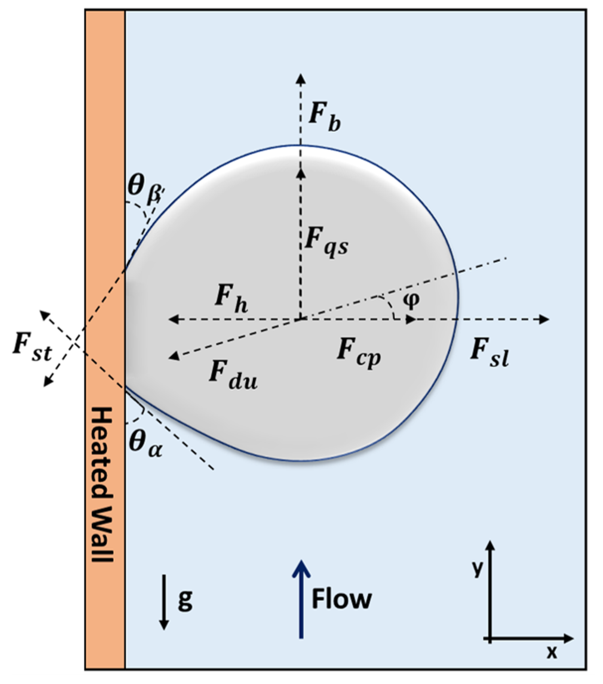
2.3. Momentum Closures

Interfacial momentum transfer has been modeled according to Ioilev formulation considering the flow pattern transition [15]. The drag force is modeled using Ishii and Zuber’s [46] model. The lift force has not been considered due to the inapplicability of the available lift coefficients. The use of lift coefficients available in the literature resulted in a substantially high near-wall void fraction compared to the experimental results [47]. The turbulent fluctuations in the continuous phase help in the redistribution of the dispersed phase and are modeled using turbulent dispersion force. The model developed by Burns et al. [48] was widely used for modeling turbulent dispersion force [7,8,9]. Hence, the Burns turbulent dispersion force model has been used in this study.

2.4. Turbulence Closure

In this study, the standard mixture $k-\epsilon$ model with enhanced wall treatment has been used for modeling turbulence. Previously, Zhang et al. [49] have shown that the standard and realizable $k-\epsilon$ models with enhanced wall treatment performed well in simulating the boiling in vertical pipe flows. Moreover, the influence of the dispersed phase on the continuous phase has been modeled using Sato et al. [50] model, and it becomes more relevant under high quality (near saturation) conditions where the vapor fraction is considerable in the center of the channel compared to highly subcooled flows.

3. Benchmark Data

CFD model validation has been carried out in two stages; in the first stage, the model has been benchmarked against the tubular DNB experimental data. Subsequently, the model has been validated against the rod bundle DNB data.

Thompson and Macbeth [21] complied tubular DNB data, out of which 20 points have been selected for this analysis. Flow boiling DNB simulations have been performed for vertical heated tubes of 7.7 and 11 mm inner diameter at high pressure and high mass flux conditions (13.8 MPa and 1351–2715 kg/m²s) using water as a coolant. The length of the tube is 0.4572 m.

The experimental rod bundle data [25] has been used for validation. They conducted CHF experiments in the High-Pressure Critical Heat Flux facility at the University of Wisconsin-Madison (UW-HPCHF) for a prototypic SMR design under high pressure and low mass flux conditions. They performed experiments in 2 × 2 fuel assembly with a 2 m heated length. The diameter of the fuel rod is 9.5 mm. Pitch to diameter is a ratio is 1.33, rod to rod, and rod to wall gap are 3.1 mm and 2.3 mm, respectively. Four small and sparsely located non-mixing vane grid spacers were used to provide support to the rod bundle. Experiments were conducted using a non-uniform axial power profile given by the following expression:

$$\frac{q\left(z\right)}{q_{avg}}={\theta }_0+{\theta }_1\cos \left(2{\theta }_2\left[\frac{z}{L}-0.5\right]\right)$$

(11)

where, $q_{avg}$ is the average heat power, $q\left(z\right)$ is the local power, z is the axial location (position—along the length of the channel/rod bundle), L is the length, ${\theta }_0$, ${\theta }_1$ and ${\theta }_2$ are 0.82, 0.68 and 2.44 respectively. A uniform radial power profile has been used in their experiments. According to Duarte et al. [25], the total power error is about 2%. From their database, in the interest of PWR, four cases have been selected for validation.

Table 3. Benchmark data (for square lattice).

S No.	Inlet Subcooling Enthalpy (kJ/kg)	Inlet Pressure (MPa)	Mass Flux (kg/m2s)	Average DNB ${\mathit{q}}_{\mathit{a}\mathit{v}\mathit{g}}^{″}$ (MW/m2)
Case-1	343	16.1	1514	1.30
Case-2	387	13.4	1526	1.58
Case-3	425	14.2	1505	1.58
Case-4	416	16.0	1506	1.44

shows the details of test cases.

DNB simulations have been carried out on a rod bundle with a hexagonal lattice. Due to a lack of experimental data, DNB simulations have been compared with Look-up tables [5,6]. The mass flux has been varied from 1500 to 3000 kg/m²s while keeping the inlet temperature at 560 K. The pressure conditions have been chosen based on the experimental study of DNB in tubes by Thompson and Macbeth [21], which is 13.8 MPa. The diameter and pitch of the hexagonal lattice are 9.4 mm and 13.1 mm, respectively. The hydraulic diameter is 11 mm.

4. Modeling Strategy

Semi-mechanistic models have been used to determine bubble departure diameter and departure frequency. Li et al. [44] model has been used for nucleation site density. The second-order upwind spatial discretization scheme has been used for the momentum, void fraction, and energy formulation. The summary of the CFD model is tabulated in

Table 4. Summary of CFD model.

CFD Solver	Euler-Euler Two Phase Solver
Turbulence model	$k-\epsilon$ model with enhanced wall treatment
Boiling Closures
Bubble Departure Diameter	Force balance model
Bubble Departure Frequency	Force balance model
Nucleation site density	Li et al. [44]
Area Influence Coefficient	Del Valle and Kenning [45]
Momentum Closures
Drag force	Ishii and Zuber [46]
Turbulent Dispersion force	Burns et al. [48]
Boundary Conditions
Inlet	Velocity inlet
Outlet	Pressure Outlet
Wall	Neumann condition (specified heat flux)
Solution Procedure
Algorithm	Coupled
Schemes	2nd order upwind for void distribution, momentum, energy, turbulent kinetic energy, and dissipation.

.

Firstly, the simulation has been initialized with a low heat flux value to ensure numerical convergence. It is executed for sufficient iterations until it reaches a converged steady-state solution. Subsequently, the heat flux has been increased in small steps, and the solution is allowed to converge at each heat flux. This process of increasing the heat flux has been repeated till an abrupt rise in wall temperature, indicating the occurrence of DNB. Figure 3 shows a typical DNB plot.

For all the cases investigated in this study, the y+ is in the range of 50–150. While maintaining the near-wall mesh size at 0.25 mm, bulk mesh size has been varied. Further refinement of near-wall mesh led to stability issues. Such stability issues were also reported previously by other researchers [14,51].

For tubular geometry, two-dimensional axis-symmetric simulations have been carried out to simulate DNB. In addition, three-dimensional CFD simulations have been performed for rod bundle simulations. The schematic of the cross-sectional geometry of the computational domain for square lattice is shown in Figure 4. The 2 × 2-rod bundles have been simulated using two symmetry boundary conditions and two wall boundary conditions, as shown in Figure 4. The effect of non-mixing vane spacers has not been considered as the spacers were small and sparsely placed. Three different meshes (1.5 million, 2.5 million, 3 million) have been considered, and no significant difference has been observed in the results.

Hexagonal subchannel cross-sectional geometry and boundary conditions are shown in Figure 5. A mesh independence study has been performed for hexagonal lattice considering three different meshes (80,000 cells, 160,000 cells, 320,000 cells), and no significant difference in DNB has been observed in the results.

The details of mesh sizes used for both types of rod bundles are tabulated in

Table 5. Grid sensitivity study for hexagonal and square rod bundles.

	Grid Size	Average Heat Flux at DNB		Deviation (%)
		Prediction (MW/m2)	Experimental (MW/m2)
Square assembly (Case 1)	~1.5 million (187 × 4000)	1.15	1.30	11.5
	~2.5 million (306 × 4000)	1.14	1.30	12.3
	~3 million (187 × 8000)	1.15	1.30	11.5
	Grid Size	Average Heat Flux at DNB		Deviation (%)
		Prediction (MW/m2)	Look-Up Table (MW/m2)
Hexagonal assembly (G = 3000 kg/m2s)	~0.08 million (180 × 425)	4.10	3.58	14.5
	~0.16 million (378 × 425)	4.02	3.58	12.3
	~0.32 million (378 × 850)	4.01	3.58	12.0

. The representative figures for mesh distribution for the computational domains of both square and hexagonal rod bundles are shown in Figure 6.

5. Results and Discussions

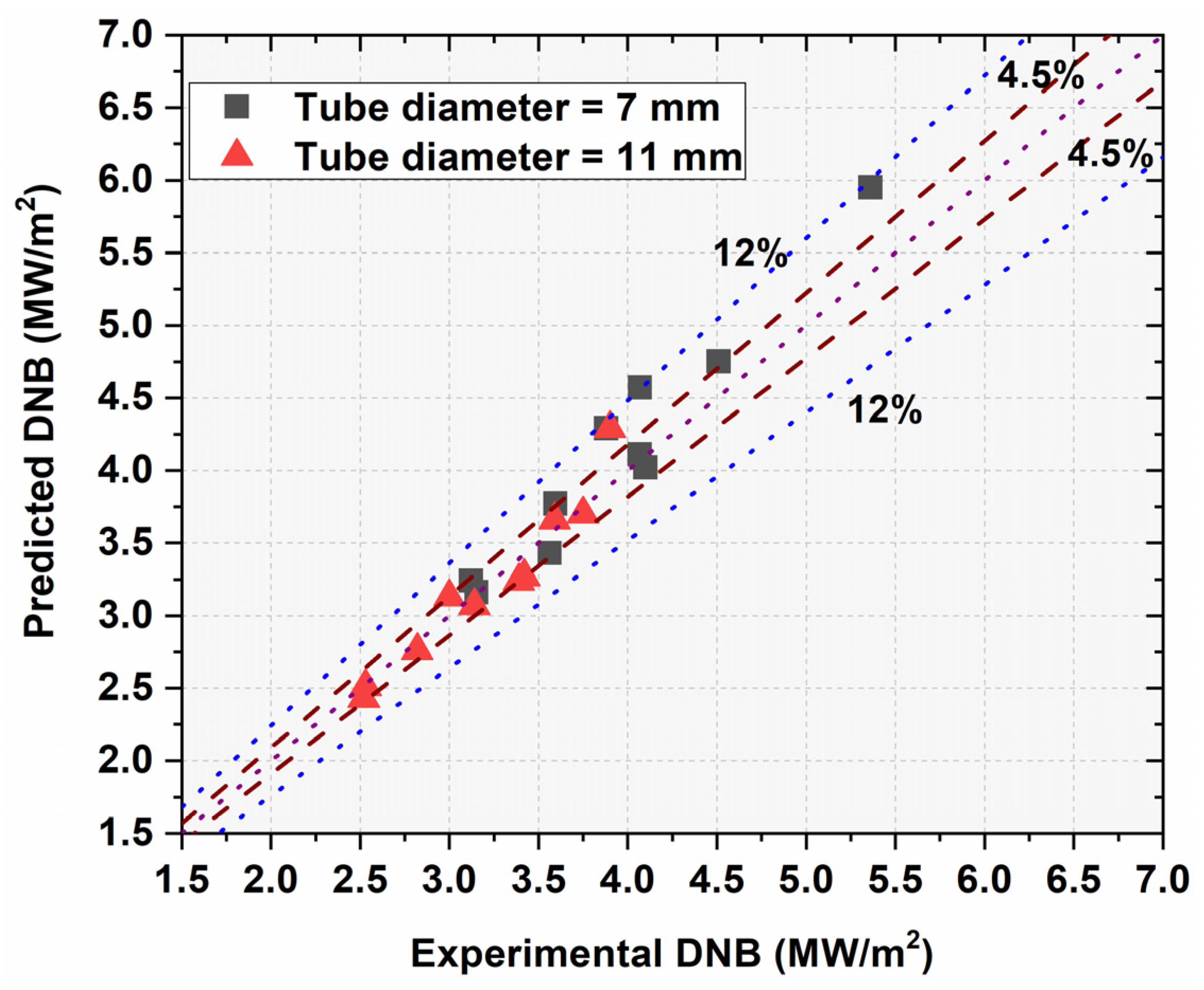
Using the methodology mentioned in Section 4, DNB numerical simulations have been carried out in tubes and rod bundles.

5.1. DNB in Tubes

Figure 7 shows the comparison between predicted DNB in this study and experimental DNB data [21] for tubes. It can be observed from Figure 7 that the maximum and mean errors are 12% and 4.5%, respectively, as opposed to the mean error of 7% and maximum error of 15% using the empirical models [24]. A typical void contour at DNB is shown in Figure 8.

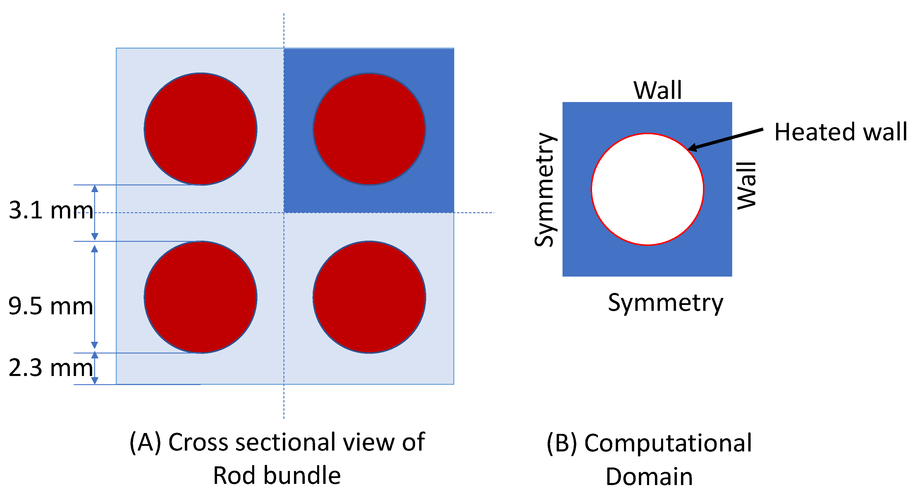
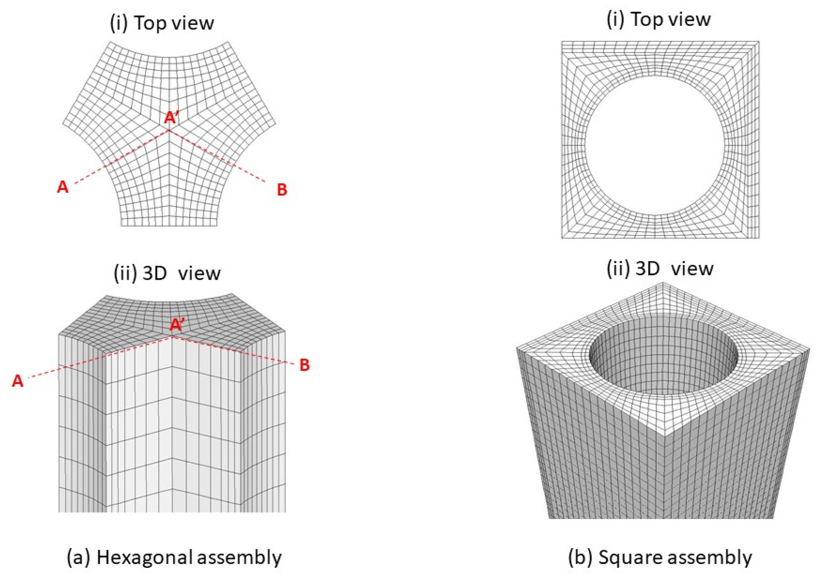
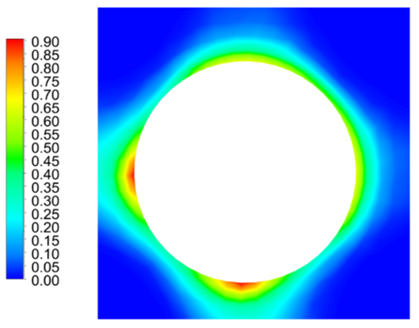
5.2. DNB in Rod Bundle (Square Lattice)

As mentioned in Section 4, three-dimensional simulations have been carried out to determine DNB in the rod bundles. CFD model predicted average heat flux at which DNB occurred with a minimum error of 11.5% and a maximum error of 19.6% compared to experimental average heat flux values (refer to

Table 6. Comparison of experimental data and predicted DNB data.

Case No.	Inlet Subcooling Enthalpy (kJ/kg)	Inlet Pressure (MPa)	Mass Flux (kg/m2s)	Average DNB ${\mathit{q}}_{\mathit{a}\mathit{v}\mathit{g}}^{″}$ (MW/m2)	Predicted ${\mathit{q}}_{\mathit{a}\mathit{v}\mathit{g}}^{″}$ (MW/m2)	Absolute Error (%)
Case-1	343	16.1	1514	1.30	1.15	11.5
Case-2	387	13.4	1526	1.58	1.27	19.6
Case-3	425	14.2	1505	1.58	1.32	16.4
Case-4	416	16.0	1506	1.44	1.27	11.8

). This result proves the CFD model’s capability to predict DNB for complex geometries and varying heat flux profiles with very good accuracy.

A typical contour at the location of DNB is shown in Figure 9. It can be observed from the void fraction contour that DNB occurred in between the rods, where the rod to rod gap has been minimum. Moreover, azimuthal variation in near-wall void fraction can be explained in detail by understanding the partitioning of heat flux.

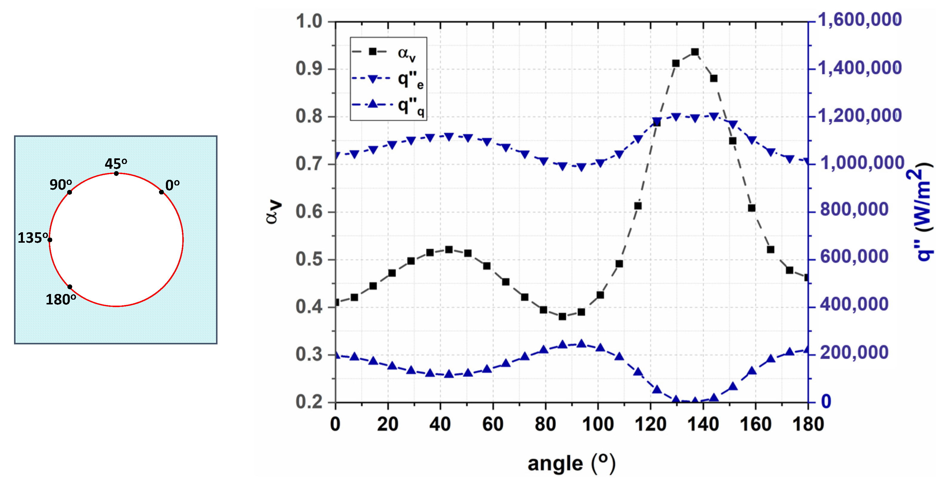
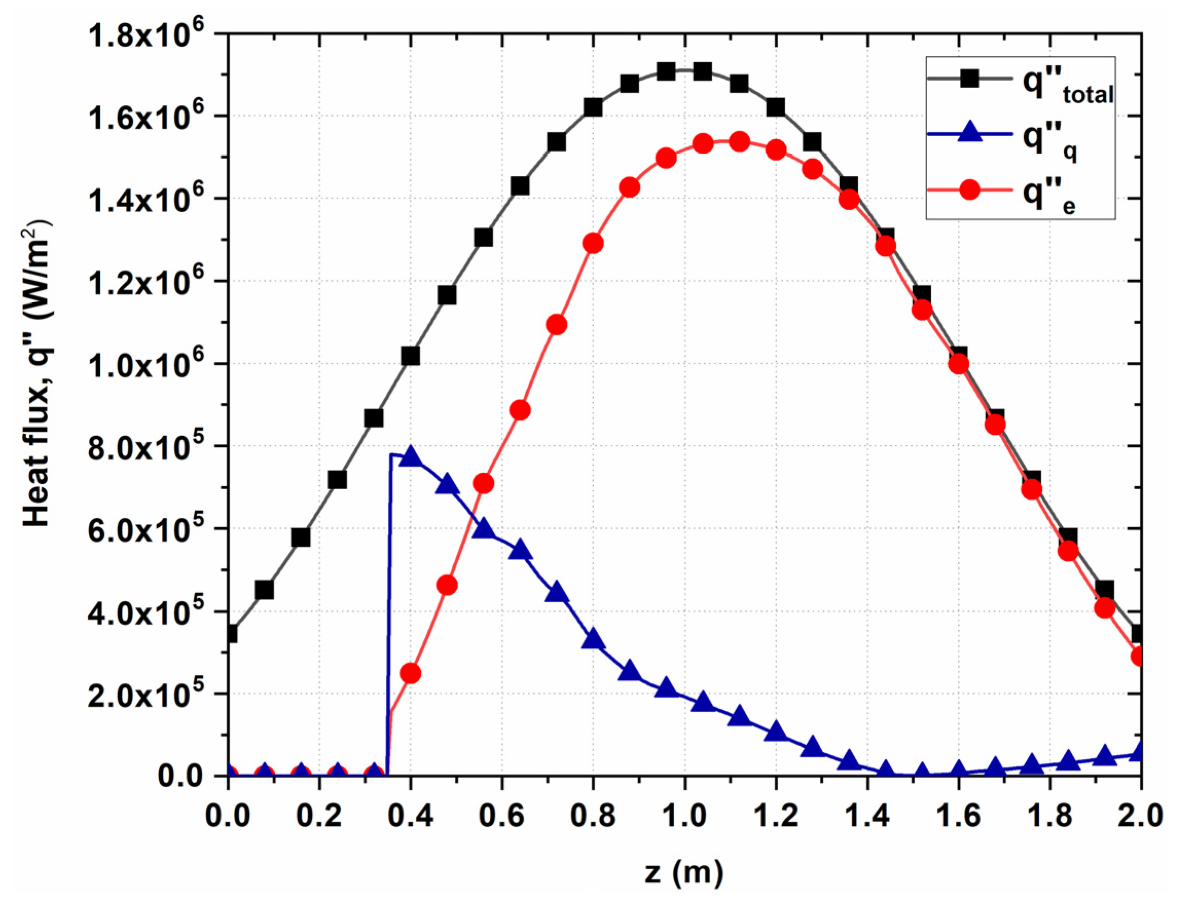
Heat Flux Partitioning Analysis

The rate of vapor generation depends on the partitioning of the wall heat flux. Unlike tubes, the near-wall void fraction can vary azimuthally in rod bundles, mainly due to differences in heat flux partitioning. Figure 10 shows the azimuthal variation of near-wall void fraction, evaporative heat flux, and quenching heat flux at the axial location where DNB has been predicted (1.48 m) for case-1 at 1.14 MW/m².

The near-wall void fraction at 135° (where the gap between the rods is minimum) is considerably higher than in other locations. Moreover, the evaporative and quenching heat fluxes follow an opposite trend to each other.

Figure 11 shows the axial variation of applied wall heat flux along with evaporative and quenching heat fluxes at an azimuthal angle of 135°. Figure 12 shows the axial variation in the near-wall void fraction along with applied heat flux at an azimuthal angle of 135°. The onset of nucleate boiling (ONB) has been predicted to occur at about 0.3 m. At the onset, the quenching heat flux is significantly higher than evaporative heat flux. However, after ONB, the evaporative heat flux follows the same trend as applied heat flux, whereas quenching heat flux follows the reverse trend. When the applied heat flux increases, the contribution of quenching heat flux reduces substantially. The decrease in quench heat flux is mainly due to the increase in liquid temperature near the wall.

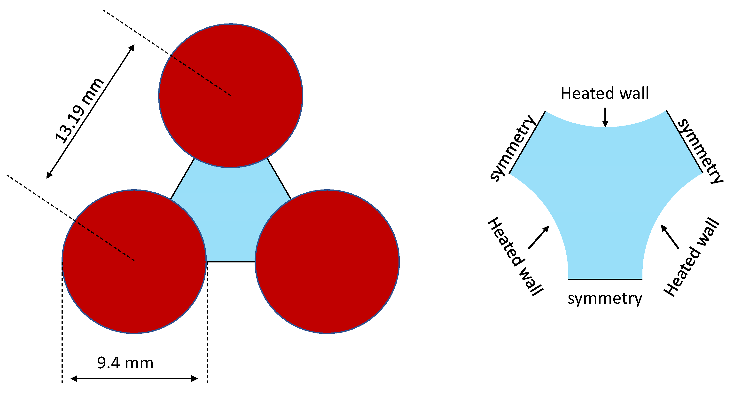
5.3. DNB in Rod Bundle (Hexagonal Lattice)

As mentioned earlier, due to the lack of experimental data for hexagonal lattice, the calculated DNB values have been compared against Look-up tables [5,6].

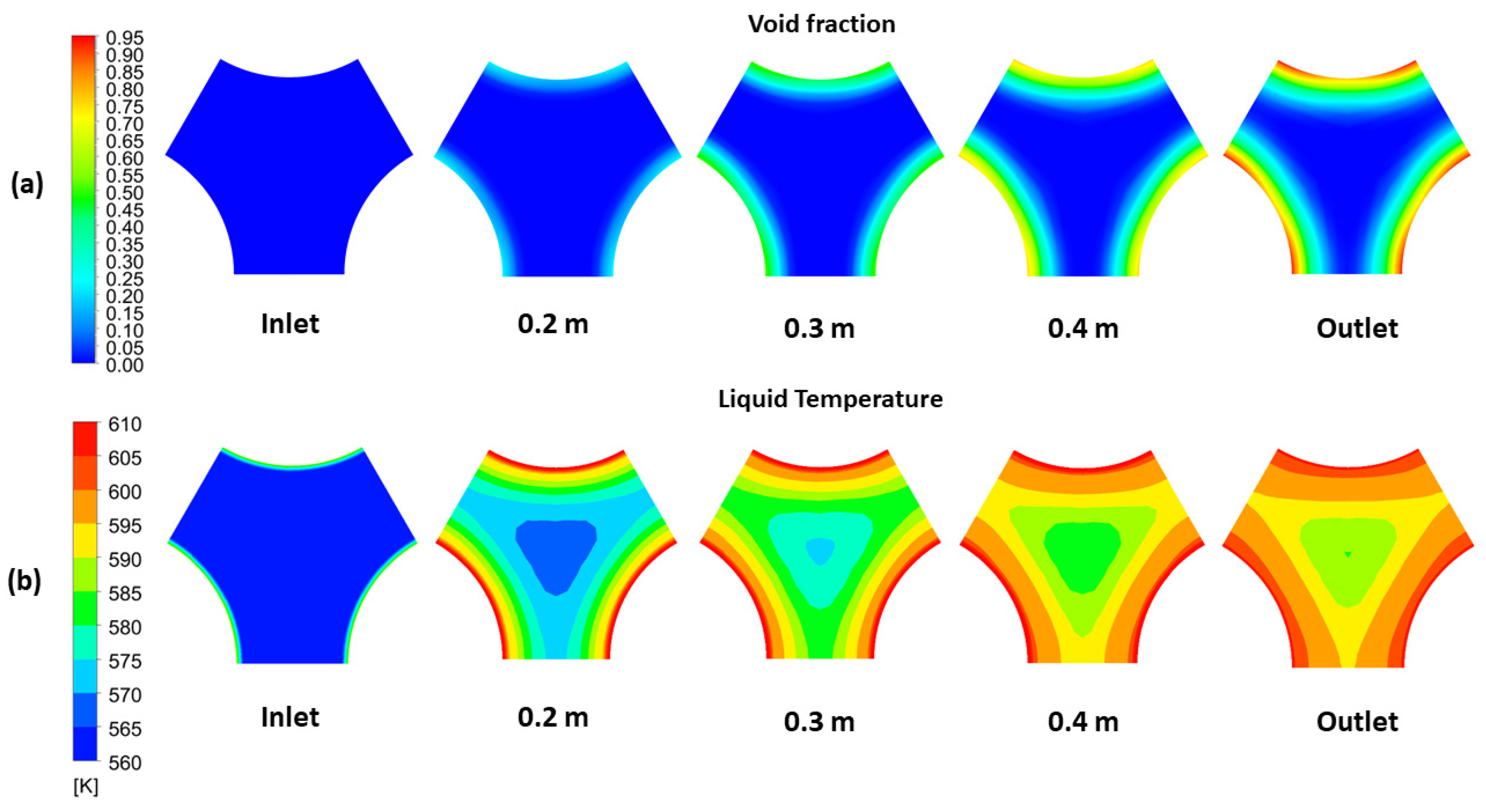
5.3.1. Void and Temperature Distribution in the Hexagonal Lattice

At multiple axial locations, vapor void fraction and liquid temperature contours corresponding to a heat flux close to DNB are shown in Figure 13. For this analysis, mass flux and inlet temperature have been considered to be 2000 kg/m²s and 560 K, respectively.

In the subchannel, liquid availability for vapor condensation is less between the rods (where the distance between rods is minimum). Consequently, the liquid temperature increases faster in that region than in the subchannel center (Figure 13b). Due to an increase in temperature, condensation decreased, resulting in significant voiding and eventually leading to DNB (Figure 13a). Hence, the DNB occurred at the radial locations where the gap between the rods is minimum. It can also be observed from Figure 13b that at all axial locations, the near-wall void fraction varies azimuthally, unlike tubular geometries.

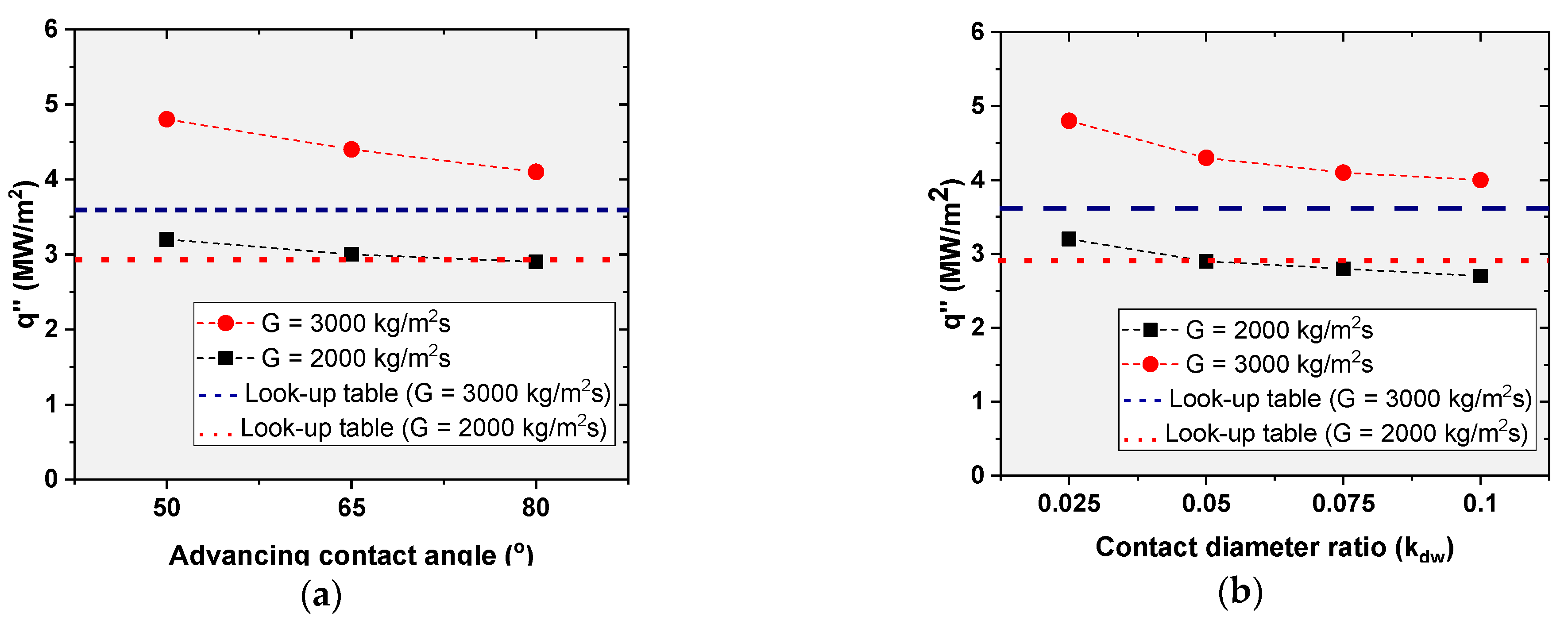
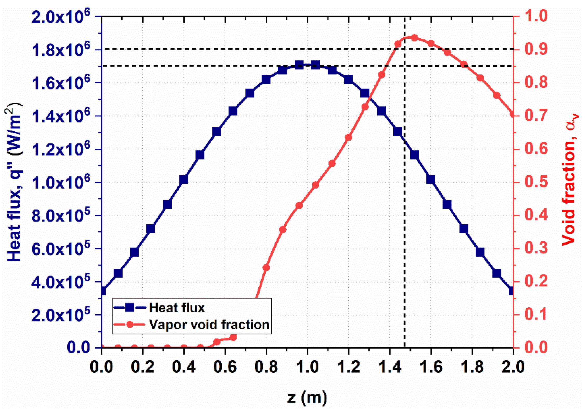
5.3.2. Comparison of Predicted DNB Values with Lookup Table

DNB values have been determined using two widely used Look-up tables available in the open literature, Groeneveld et al. [5] and Bobkov et al. [6]. The heat balance method has been used to determine DNB values using Look-up tables with appropriate correction factors. Details about the Look-up tables and correction factors have been discussed in detail in Appendix A. DNB values have been calculated using the CFD model and compared with Look-up table data. The deviations from Look-up data predictions are tabulated along with the CFD calculation in

Table 7. Comparison of predicted DNB to Look-up table [1,2] data.

Mass Flux (kg/m2s)	Predicted DNB (MW/m2)	Groeneveld Look-Up Table DNB (MW/m2)	Bobkov Look-Up Table (MW/m2)	Deviation from Groeneveld (%)	Deviation from Bobkov (%)
1500	2.23	2.43	2.54	8.2	12.2
2000	2.87	2.82	2.97	1.8	3.4
2500	3.45	3.18	3.28	8.5	5.2
3000	4.02	3.53	3.58	13.9	12.3

. The maximum deviation of CFD calculations has been found to be 13.9% from Groeneveld’s Look-up table, and 12.3%from Bobkov’s Look-up when the mass flux is 3000 kg/m²s. It is also clear from Table 7 that both Look-up tables deviate from each other slightly.

6. Conclusions

In this present work, DNB has been modeled using the EEHFP model with semi-mechanistic models for determining bubble departure characteristics (bubble departure diameter and departure frequency). A comprehensive CFD analysis has been carried out to assess the capability of the EEHFP model to determine DNB in tubes and rod bundles. The semi-mechanistic model relies on a more physics-backed approach based on force balance analysis. The results have shown that using such models, the error in DNB prediction reduced substantially. The specific conclusions drawn from the present study are as below,

• Using the developed semi-mechanistic models for bubble departure characteristics, DNB has been predicted in tubes at high-pressure conditions with a mean error of 4.5% and maximum error of 12%, as opposed to the mean error of 7% and maximum error of 15% using the empirical models [24].
• The CFD model predicted the average heat flux at which DNB occurred with a minimum error of 11.5% and a maximum error of 19.6% compared to experimental average heat flux values in square lattices.
• CFD model has also been used to predict DNB in hexagonal subchannel at various mass flux values at 13.8 MPa. Predicted DNB values of hexagonal subchannel have been compared with both Bobkov and Groeneveld Look-up tables with appropriate correction factors. Predicted DNB deviations have been in the range of 1.8–13.9% for hexagonal lattices.

Overall, the model under current consideration proved capable of predicting DNB values in rod bundles with reasonable accuracy. Incorporating semi-mechanistic models for determining bubble departure characteristics within the framework of heat flux partitioning proved to be an effective method in predicting the DNB in tubes and rod bundles.

However, the models are required for many crucial parameters like contact angles and contact diameters to reduce empiricism and improve confidence in this approach. Therefore, future models and experiments should reduce the empiricism involved in those parameters. Moreover, proper quantification of heat transfer due to sliding bubbles at high-pressure conditions is required. As the bubbles slide, they may disturb the thermal boundary layer. Furthermore, improvement in the modeling of interfacial forces is required to increase the reliability of the CFD model. Mainly, the lift force model should be developed to consider the effect of the swarm of bubbles at high-pressure conditions.

References

1. Todreas, N.E.; Kazimi, M.S. Nuclear Systems Volume I: Thermal Hydraulic Fundamentals; CRC Press, Taylor & Francis Group: Boca Raton, FL, USA, 2012. [Google Scholar]
2. Hall, D.D.; Mudawar, I. Critical Heat Flux (CHF) for Water Flow in Tubes-I. Compilation and Assessment of World CHF Data. Int. J. Heat Mass Transf. 2000, 43, 2573–2604. [Google Scholar] [CrossRef]
3. Reddy, D.G.; Fighetti, C.F. Parametric Study of CHF Data. Volume 2. A Generalized Subchannel CHF Correlation for PWR and BWR Fuel Assemblies; Final Report No. EPRI-NP-2609-Vol. 2; Department of Chemical Engineering, Columbia University: New York, NY, USA, 1983. [Google Scholar]
4. Hall, D.D.; Mudawar, I. Critical Heat Flux (CHF) for Water Flow in Tubes—II. Int. J. Heat Mass Transf. 2000, 43, 2605–2640. [Google Scholar] [CrossRef]
5. Groeneveld, D.C.; Shan, J.Q.; Vasić, A.Z.; Leung, L.K.H.; Durmayaz, A.; Yang, J.; Cheng, S.C.; Tanase, A. The 2006 CHF Look-up Table. Nucl. Eng. Des. 2007, 237, 1909–1922. [Google Scholar] [CrossRef]
6. Bobkov, V.P.; Efanov, A.D.; Pomet’ko, R.S.; Smogalev, I.P. A Modified Table for Calculating Critical Heat Fluxes in Assemblies of Triangularly Packed Fuel Rods. Therm. Eng. 2011, 58, 317–324. [Google Scholar] [CrossRef]
7. Krepper, E.; Rzehak, R. CFD for Subcooled Flow Boiling: Simulation of DEBORA Experiments. Nucl. Eng. Des. 2011, 241, 3851–3866. [Google Scholar] [CrossRef]
8. Krepper, E.; Končar, B.; Egorov, Y. CFD Modelling of Subcooled Boiling—Concept, Validation and Application to Fuel Assembly Design. Nucl. Eng. Des. 2007, 237, 716–731. [Google Scholar] [CrossRef]
9. Colombo, M.; Fairweather, M. Accuracy of Eulerian–Eulerian, Two-Fluid CFD Boiling Models of Subcooled Boiling Flows. Int. J. Heat Mass Transf. 2016, 103, 28–44. [Google Scholar] [CrossRef]
10. Murallidharan, J.S.; Prasad, B.V.S.S.S.; Patnaik, B.S.V.; Hewitt, G.F.; Badalassi, V. CFD Investigation and Assessment of Wall Heat Flux Partitioning Model for the Prediction of High Pressure Subcooled Flow Boiling. Int. J. Heat Mass Transf. 2016, 103, 211–230. [Google Scholar] [CrossRef]
11. Baglietto, E.; Demarly, E.; Kommajosyula, R.; Lubchenko, N.; Magolan, B.; Sugrue, R. A Second Generation Multiphase-CFD Framework Toward Predictive Modeling of DNB. Nucl. Technol. 2019, 205, 1–22. [Google Scholar] [CrossRef]
12. Tentner, A.; Lo, S.; Ioilev, A.; Melnikov, V.; Samigulin, M.; Ustinenko, V.; Kozlov, V. Advances in Computational Fluid Dynamics Modeling of Two Phase Flow in a Boiling Water Reactor Fuel Assembly. In Proceedings of the International Conference on Nuclear Engineering, Miami, FL, USA, 17–20 July 2006. [Google Scholar]
13. Lavieville, J.; Quemerais, E.; Mimouni, S.; Boucker, M.; Mechitoua, N. NEPTUNE CFD V1. 0 Theory Manual. Rainterne EDF H-I81-2006-04377-EN. RaNEPTUNE Nept_2004_L, 1. Available online: https://scholar.google.com/scholar_lookup?hl=en&publication_year=2006&author=J.+Lavieville&title=NEPTUNE+CFD+V1.+0+theory+manual (accessed on 16 December 2021).
14. Zhang, R.; Cong, T.; Tian, W.; Qiu, S.; Su, G. Prediction of CHF in Vertical Heated Tubes Based on CFD Methodology. Prog. Nucl. Energy 2015, 78, 196–200. [Google Scholar] [CrossRef]
15. Ioilev, A.; Samigulin, M.; Ustinenko, V.; Kucherova, P.; Tentner, A.; Lo, S.; Splawski, A. Advances in the Modeling of Cladding Heat Transfer and Critical Heat Flux in Boiling Water Reactor Fuel Assemblies. In Proceedings of the 12th International Topical Meeting on Nuclear Reactor Thermal Hydraulics (NURETH-12), Pittsburgh, PA, USA, 30 September–4 October 2007. [Google Scholar]
16. Li, Q.; Avramova, M.; Jiao, Y.; Chen, P.; Yu, J.; Pu, Z.; Chen, J. CFD Prediction of Critical Heat Flux in Vertical Heated Tubes with Uniform and Non-Uniform Heat Flux. Nucl. Eng. Des. 2018, 326, 403–412. [Google Scholar] [CrossRef]
17. Kim, S.J.; Baglietto, E.; Demarly, E. Evaluation of DNB Predictive Capability in Multiphase Boiling Model of STAR-CCM+; Los Alamos National Lab. (LANL): Los Alamos, NM, USA, 2018.
18. Kim, S.J. Assessment on DNB Performance for High Pressure Subcooled Boiling with Modified CASL Boiling Model; Los Alamos National Laboratory: Los Alamos, NM, USA, 2019.
19. Sugrue, R.M. A Robust Momentum Closure Approach for Multiphase Computational Fluid Dynamics Applications. Ph.D. Thesis, Massachusetts Institute of Technology, Boston, MA, USA, 2017. [Google Scholar]
20. Lubchenko, N.; Magolan, B.; Sugrue, R.; Baglietto, E. A More Fundamental Wall Lubrication Force from Turbulent Dispersion Regularization for Multiphase CFD Applications. Int. J. Multiph. Flow 2018, 98, 36–44. [Google Scholar] [CrossRef]
21. Thompson, B.; Macbeth, R.V. Boiling Water Heat Transfer Burnout in Uniformly Heated Round Tubes: A Compilation of World Data with Accurate Correlations; No. AEEW-R-356, United Kingdom Atomic Energy Authority, Reactor Group; Atomic Energy Establishment: Winfrith, UK, 1964.
22. Xu, Y.; Brewster, R.A.; Conner, M.E.; Karoutas, Z.E.; Smith, L.D. CFD Modeling Development for DNB Prediction of Rod Bundle with Mixing Vanes Under PWR Conditions. Nucl. Technol. 2019, 205, 57–67. [Google Scholar] [CrossRef]
23. Zhang, R.; Duarte, J.P.; Cong, T.; Corradini, M.L. Investigation on the Critical Heat Flux in a 2 by 2 Fuel Assembly under Low Flow Rate and High Pressure with a CFD Methodology. Ann. Nucl. Energy 2019, 124, 69–79. [Google Scholar] [CrossRef]
24. Vadlamudi, S.R.G.; Nayak, A.K. CFD Simulation of Departure from Nucleate Boiling in Vertical Tubes under High Pressure and High Flow Conditions. Nucl. Eng. Des. 2019, 352, 110150. [Google Scholar] [CrossRef]
25. Duarte, J.P.; Zhao, D.; Jo, H.; Corradini, M.L. Critical Heat Flux Experiments and a Post-CHF Heat Transfer Analysis Using 2D Inverse Heat Transfer. Nucl. Eng. Des. 2018, 337, 17–26. [Google Scholar] [CrossRef]
26. Ishii, M.; Hibiki, T. Thermo-Fluid Dynamics of Two-Phase Flow; Springer Science & Business Media: New York, NY, USA, 2010. [Google Scholar]
27. Klausner, J.F.; Mei, R.; Bernhard, D.M.; Zeng, L.Z. Vapor Bubble Departure in Forced Convection Boiling. Int. J. Heat Mass Transf. 1993, 36, 651–662. [Google Scholar] [CrossRef]
28. Tolubinsky, V.I.; Kostanchuk, D.M. Vapour Bubbles Growth Rate and Heat Transfer Intensity at Subcooled Water Boiling. In Proceedings of the International Heat Transfer Conference 4, Begellhouse, CT, USA, 31 August–5 September 1970; pp. 1–11. [Google Scholar]
29. Yun, B.-J.; Splawski, A.; Lo, S.; Song, C.-H. Prediction of a Subcooled Boiling Flow with Advanced Two-Phase Flow Models. Nucl. Eng. Des. 2012, 253, 351–359. [Google Scholar] [CrossRef]
30. Sugrue, R.; Buongiorno, J. A Modified Force-Balance Model for Prediction of Bubble Departure Diameter in Subcooled Flow Boiling. Nucl. Eng. Des. 2016, 305, 717–722. [Google Scholar] [CrossRef]
31. Colombo, M.; Fairweather, M. Prediction of Bubble Departure in Forced Convection Boiling: A Mechanistic Model. Int. J. Heat Mass Transf. 2015, 85, 135–146. [Google Scholar] [CrossRef]
32. Kurul, N.; Podowski, M.Z. Multidimensional Effects in Forced Convection Subcooled Boiling. In Proceedings of the 9th International Heat Transfer Conference, Jerusalem, Israel, 19–24 August 1990; pp. 21–26. [Google Scholar]
33. Collier, J.G.; Thome, J.R. Convective Boiling and Condensation; Clarendon Press: Oxford, UK, 1994. [Google Scholar]
34. Tong, L.S.; Tang, Y.S. Boiling Heat Transfer and Two-Phase Flow; Series in Chemical and Mechanical Engineering; Taylor and Francis: Washington, DC, USA, 1997. [Google Scholar]
35. Mikic, B.; Rohsenow, W.; Griffith, P. On Bubble Growth Rates. Int. J. Heat Mass Transf. 1970, 13, 657–666. [Google Scholar] [CrossRef]
36. Forster, H.K.; Zuber, N. Growth of a Vapor Bubble in a Superheated Liquid. J. Appl. Phys. 1954, 25, 474–478. [Google Scholar] [CrossRef]
37. Cooper, M.G. The Microlayer and Bubble Growth in Nucleate Pool Boiling. Int. J. Heat Mass Transf. 1969, 12, 915–933. [Google Scholar] [CrossRef]
38. Sakashita, H. Bubble Growth Rates and Nucleation Site Densities in Saturated Pool Boiling of Water at High Pressures. J. Nucl. Sci. Technol. 2011, 48, 734–743. [Google Scholar] [CrossRef]
39. Murallidharan, J.; Giustini, G.; Sato, Y.; Ničeno, B.; Badalassi, V.; Walker, S.P. Computational Fluid Dynamic Simulation of Single Bubble Growth under High-Pressure Pool Boiling Conditions. Nucl. Eng. Technol. 2016, 48, 859–869. [Google Scholar] [CrossRef] [Green Version]
40. Plesset, M.S.; Zwick, S.A. The Growth of Vapor Bubbles in Superheated Liquids. J. Appl. Phys. 1954, 25, 493–500. [Google Scholar] [CrossRef] [Green Version]
41. Vadlamudi, S.R.G.; Nayak, A.K. The Influence of Bubble Departure Characteristics on CHF Prediction at High-Pressure Conditions. Case Stud. Therm. Eng. 2020, 22, 100735. [Google Scholar] [CrossRef]
42. Kocamustafaogullari, G.; Ishii, M. Interfacial Area and Nucleation Site Density in Boiling Systems. Int. J. Heat Mass Transf. 1983, 26, 1377–1387. [Google Scholar] [CrossRef]
43. Hibiki, T.; Ishii, M. Active Nucleation Site Density in Boiling Systems. Int. J. Heat Mass Transf. 2003, 46, 2587–2601. [Google Scholar] [CrossRef]
44. Li, Q.; Jiao, Y.; Avramova, M.; Chen, P.; Yu, J.; Chen, J.; Hou, J. Development, Verification and Application of a New Model for Active Nucleation Site Density in Boiling Systems. Nucl. Eng. Des. 2018, 328, 1–9. [Google Scholar] [CrossRef]
45. Del Valle, V.H.; Kenning, D.B.R. Subcooled Flow Boiling at High Heat Flux. Int. J. Heat Mass Transf. 1985, 28, 1907–1920. [Google Scholar] [CrossRef]
46. Ishii, M.; Zuber, N. Drag Coefficient and Relative Velocity in Bubbly, Droplet or Particulate Flows. AIChE J. 1979, 25, 843–855. [Google Scholar] [CrossRef]
47. Vadlamudi, S.R.G.; Nayak, A.K. Investigations on Effect of Lift and Wall Lubrication Forces on the Subcooled Flow Boiling. ASME J. Nucl. Eng. Radiat. Sci. 2020, 6, 041109. [Google Scholar] [CrossRef]
48. Burns, A.D.; Frank, T.; Hamill, I.; Shi, J.-M.M. The Favre Averaged Drag Model for Turbulent Dispersion in Eulerian Multi-Phase Flows. In Proceedings of the 5th International Conference on Multiphase Flow, ICMF-2004, Yokohama, Japan, 30 May–4 June 2004; pp. 1–17. [Google Scholar]
49. Zhang, R.; Cong, T.; Tian, W.; Qiu, S.; Su, G. Effects of Turbulence Models on Forced Convection Subcooled Boiling in Vertical Pipe. Ann. Nucl. Energy 2015, 80, 293–302. [Google Scholar] [CrossRef]
50. Sato, Y.; Sadatomi, M.; Sekoguchi, K. Momentum and Heat Transfer in Two-Phase Bubble Flow—I. Theory. Int. J. Multiph. Flow 1981, 7, 167–177. [Google Scholar] [CrossRef]
51. Kim, S.J.; Johns, R.C.; Yoo, J.; Baglietto, E. Progress Toward Simulating Departure from Nucleate Boiling at High-Pressure Applications with Selected Wall Boiling Closures. Nucl. Sci. Eng. 2020, 194, 690–707. [Google Scholar] [CrossRef]
52. Groeneveld, D.C.; Cheng, S.C.; Doan, T. 1986 AECL-UO Critical Heat Flux Lookup Table. Heat Transf. Eng. 1986, 7, 46–62. [Google Scholar] [CrossRef]
53. Groeneveld, D.C.; Leung, L.K.H.; Guo, Y.; Vasic, A.; El Nakla, M.; Peng, S.W.; Yang, J.; Cheng, S.C. Lookup Tables for Predicting CHF and Film-Boiling Heat Transfer: Past, Present, and Future. Nucl. Technol. 2005, 152, 87–104. [Google Scholar] [CrossRef]
Figure 1. Schematic of forces acting on a bubble.
Fluids 07 00083 g001
Figure 2. (a,b) represent variation in predicted DNB value with different advancing contact angles and contact diameter ratios, respectively. The values predicted by the Look-up table [5] are also plotted for reference. (adapted from Vadlamudi and Nayak [41]).
Fluids 07 00083 g002
Figure 3. Evolution of wall temperature with iterations.
Fluids 07 00083 g003
Figure 4. Geometry and boundary conditions (square lattice).
Fluids 07 00083 g004
Figure 5. Hexagonal subchannel geometry and boundary conditions.
Fluids 07 00083 g005
Figure 6. (a): (i) top view of mesh distribution (0.16 million) in hexagonal assembly, (ii) corresponding 3D view of mesh distribution in hexagonal assembly. The portion enclosed by planes A–A’ and A’–B corresponding to the top view in (i) has been removed in (ii) to show the internal mesh distribution. (b): (i) top view of mesh distribution in square assembly (2.5 million), (ii) corresponding 3D view of mesh distribution in square assembly.
Fluids 07 00083 g006
Figure 7. Predicted DNB vs. Experimental DNB (for tubes with 7 and 11 mm diameter).
Fluids 07 00083 g007
Figure 8. Void Contour at DNB (for tubes).
Fluids 07 00083 g008
Figure 9. Typical void contour at DNB.
Fluids 07 00083 g009
Figure 10. Azimuthal variation of near-wall void fraction, evaporative heat flux, and quenching heat flux at axial DNB location (1.48 m) for case-1 at 1.14 MW/m2.
Fluids 07 00083 g010
Figure 11. Variation in total applied heat flux, evaporative heat flux, and quenching heat flux with axial length (135°).
Fluids 07 00083 g011
Figure 12. Evolution of near-wall void fraction at an azimuthal location of 135°.
Fluids 07 00083 g012
Figure 13. (a) Void fraction contours and (b) liquid temperature contours at various axial locations (inlet, 0.2 m, 0.3 m, 0.4 m, and outlet), respectively.
Fluids 07 00083 g013