A Numerical Analysis on the Unsteady Flow of a Thermomagnetic Reactive Maxwell Nanofluid over a Stretching/Shrinking Sheet with Ohmic Dissipation and Brownian Motion

Abstract

The major objective of this current investigation is to examine the unsteady flow of a thermomagnetic reactive Maxwell nanofluid flow over a stretching/shrinking sheet with Ohmic dissipation and Brownian motion. Suitable similarity transformations were used to reduce the governing non-linear partial differential equations of momentum, energy and species conservation into a set of coupled ordinary differential equations. The reduced similarity ordinary differential equations were solved numerically using the Spectral Quasi-Linearization Method. The influence of some pertinent physical parameters on the velocity, temperature and concentration distributions was studied and analysed graphically. Further investigations were made on the impact of the Eckert number, Prandtl number, Schmidt number, thermal radiation parameter, Brownian motion parameter, thermophoresis parameter and chemical reaction parameter on the skin friction coefficient, surface heat and mass transfer rates. The results were displayed in a tabular form. Obtained results reveal that the Maxwell parameter and the unsteadiness parameter reduce the Maxwell nanofluid velocity and the fluid temperature is increased with an increase in the Eckert number and thermal radiation parameter.

1. Introduction

There is a growing demand for fluids with improved thermal conductivity and heat transfer properties in industrial applications which include micro-manufacturing, chemical and metallurgical, power generation, transportation, cooling, ventilation and air conditioning. The heat transfer rate achieved by commonly used cooling media such as water and air is not suitable for other industrial applications, hence the need to develop advanced heat transfer fluids. Some fluids with a high thermal conductivity can be engineered by suspending nano-sized particles in conventional heat transfer fluids such as engine oil, water, ethylene glycol, etc. The nano-sized particles (<100 nm in diameter) can be metals, carbides, oxides and carbon. The mixture of the nano-particles and the base fluid results in a new innovative fluid, coined a nanofluid by Choi and Eastman [1]. The most commonly used nanofluids are ZnO in ethylene glycol, TiO₂ in water, Al₂O₃ in water and CuO in water. Nanofluids have found applications in electronic cooling, lubrication, microelectronic fuel cells, oil recovery, drug delivery and magnetic cell separation, Jakati et al. [2].

A non-Newtonian fluid is a fluid which exhibits a non-linear relationship between the applied stress and shear rate. Typical examples of non-Newtonian fluids include biological stuff (synovial fluid, blood, syrups), chemical material (pharmaceutical chemicals, paints, tooth pastes), food products (milk, ice creams, chocolates) [3]. In the mathematical modelling of non-Newtonian fluids, it is difficult to come up with a one constitutive relationship that captures all the properties of these fluids. As a result, researchers have suggested several non-Newtonian models. Amongst these models, is the rate-type Maxwell model [4], which represents the characteristics of the fluid relaxation times. A vast range of the applications of non-Newtonian nanofluids are found in technology and industrial applications such as in paints, asphalts, tars, melts of polymers, glues and biological solutions [5].

Crane [6] conducted the pioneering work on the study of flow over a sheet which is stretching. Studying the boundary layer flow over a sheet which is stretching has quite a number of engineering and industrial applications. In particular, the study is of significance in areas such as in paper production, wire drawing, extrusion processes, cooling of metallic plate in a bath, food processing and movement of biological fluids. Khan et al. [7] employed the homotopy analysis method to study heat and mass transfer of a Carreau fluid flowing past a stretching surface. Kudenatti and Misbah [8] reported on a unified computational approach of a hydrodynamic power-law fluid past a stretching sheet. A study on the effect of thermal radiation on a three dimensional MHD boundary layer flow of a Jeffrey nanofluid over a non-linearly stretching sheet was performed by Gireesha et al. [9]. Shahzad et al. [10] used the Keller box method to study viscous Jeffrey nanofluid flow past a stretching sheet embedded in a porous medium. Jayachandra and Sandeep [11] used the Runge–Kutta method to study cross-diffusion effects on MHD Williamson fluid past a stretching sheet. A model to consider boundary value problems in polymer flow due to a stretching sheet was studied by Baranovskii [12]. More studies on the non-Newtonian fluid flow past a stretching sheet have been performed by [13,14,15,16].

Quite a lot of research has been conducted on the Maxwell nanofluid flow past a stretching or shrinking sheet. Prasannakumara [17] used the Runge–Kutta–Fehlberg fourth-fifth order (RKF-45) method to solve ordinary differential equations modelling heat transport in a Maxwell nanofluid flowing a stretching sheet. Hussain et al. [18] used the RKF-45 algorithm to perform a numerical and statistical analysis of graphene Maxwell nanofluid flowing past a sheet which is stretched. The implicit finite difference method was used by Ibrahim and Negera [19] to investigate the slip effects and stagnation point flows of a Maxwell nanofluid flowing over a stretching sheet. Shafiq et al. [20] used Matlab’s bvp4c to study the flow of Maxwell nanofluid over a sheet which is stretching exponentially. A semi-analytical technique homotopy analysis method was used to consider the unsteady thermal flow of the Maxwell power law nanofluid over a stretching sheet by Jawad et al. [21].

The system of partial differential equations modelling the flow of the Maxwell nanofluid flowing over a stretching sheet are solved using the Spectral Quasi-linearization Method (SQLM) [22]. It has been reported that this numerical technique needs a few seconds and iterations to provide accurate and converged results, respectively [23]. The SQLM has been used to analyse the flow behaviour of non-Newtonian fluid flow. Some of the studies include the works by Alharbey et al. [24], Magodora et al. [25], Mondal and Sibanda [26], Mondal and Bharti [27], Nayak et al. [28], Sahoo and Nandkeolyar [29]. The utilization of similarity transformations on the coupled system of non-linear partial differential equations governing the Maxwell nanofluid flow resulted in a system of non-linear ordinary differential equations which in turn were solved using SQLM. The influence of some pertinent parameters such as thermophoresis parameter, Eckert number, magnetic parameter, Prandtl number, thermal radiation parameter, Brownian motion parameter and the unsteadiness parameter on the velocity, temperature and concentration profiles were analysed. The results for the skin friction coefficient and the heat transfer rate obtained using SQLM were found to be in good agreement with those in the published literature. The reliability of the SQLM was also demonstrated by comparing the results obtained for the skin friction coefficient and the heat transfer rate with those from Matlab bvp4c [30]. An excellent agreement was established.

Based on research in the literature, it is to the best knowledge of the authors that no work has been conducted on the reactive thermomagnetic Maxwell nanofluid with Ohmic dissipation and Brownian motion. Significant merits of the recent Spectral Quasi-Linearization Method were noted in published work. This motivated the authors to use the numerical technique to analyse the current problem under study which is of utmost importance to mechanical and physical engineering applications.

2. Mathematical Formulation

In this study, the unsteady flow of a thermomagnetic reactive optically thick Maxwell nanofluid over a stretching/shrinking sheet with Ohmic dissipation and Brownian motion was analysed. The flow is in the upper region $y>0$ and has a uniform magnetic field of strength $B=\frac{B_0}{\sqrt{1-\alpha t}}$ subjected to it, with an initial magnetic field strength denoted by $B_0$. The magnetic field is applied perpendicular to the sheet. The unsteady fluid, heat and mass transfer flows are assumed to start at $t=0$. The sheet emerges at point $(x,y)=(0,0)$ moving with a non-uniform velocity $u_w(x,t)=\frac{ax}{1-\alpha t},$ where a and $\alpha$ are positive constants with inverse time dimension ${\left(time\right)}^{-1}$, and a is an initial stretching rate. The velocity of mass transfer is $v_w(x,t)=\frac{v_0}{\sqrt{1-\alpha t}},$ where $v_0$ is the constant mass flux velocity. Additionally, $T_w$ and $C_w$ are the surface temperature and concentration, respectively. Then $T_{\infty }$ and $C_{\infty }$ are their respective ambient values. In this problem, the induced magnetic field is considered negligible due to the magnetic Reynolds number in the flow which is assumed to be very small. Assumed to be negligible is the external electric field and the electric field which results from the polarization of charges. The flow diagram and coordinate system of the current problem is shown in Figure 1.

Therefore, the governing equations of such a model flow, under the usual boundary layer approximations in the usual notations are (Madhu et al.): [31]:

$$\frac{\partial u}{\partial x}+\frac{\partial v}{\partial y}=0,$$

(1)

$$\frac{\partial u}{\partial t}+u\frac{\partial u}{\partial x}+v\frac{\partial u}{\partial y}+\lambda \left(u^2\frac{{\partial }^{2}u}{\partial x^2}+v^2\frac{{\partial }^{2}u}{\partial y^2}+2uv\frac{{\partial }^{2}u}{\partial x\partial y}\right)={\nu }_f\frac{{\partial }^{2}u}{\partial y^2}+g{\beta }_f(T-T_{\infty })+g{\beta }_f^{*}(C-C_{\infty })-\frac{\sigma B^2}{{\rho }_f}u,$$

(2)

$$\frac{\partial T}{\partial t}+u\frac{\partial T}{\partial x}+v\frac{\partial T}{\partial y}=\frac{k_f}{{\left(\rho c\right)}_f}\frac{{\partial }^{2}T}{\partial y^2}-\frac{1}{{\left(\rho c\right)}_f}\frac{\partial q_r}{\partial y}+\frac{{\mu }_f}{{\left(\rho c\right)}_f}{\left(\frac{\partial u}{\partial y}\right)}^2+\frac{\sigma B^2}{{\left(\rho c\right)}_f}{u}^2+\tau \left\{D_B\frac{\partial T}{\partial y}\frac{\partial C}{\partial y}+\frac{D_T}{T_{\infty }}{\left(\frac{\partial T}{\partial y}\right)}^2\right\},$$

(3)

$$\frac{\partial C}{\partial t}+u\frac{\partial C}{\partial x}+v\frac{\partial C}{\partial y}=D_B\frac{{\partial }^{2}C}{\partial y^2}+\frac{D_T}{T_{\infty }}\frac{{\partial }^{2}T}{\partial y^2}-k_r(C-C_{\infty }),$$

(4)

where the velocities in the x and y directions are u and v respectively. $\lambda =\frac{{\lambda }_0}{1-\alpha t}$ is the relaxation parameter of the Maxwell fluid, g is the acceleration due to gravity, ${\beta }_f$ is volumetric thermal expansion, ${\beta }_f^{*}$ is volumetric solution expansion, T is the fluid temperature, C is the fluid concentration, $D_B$ is the Brownian diffusion coefficient, $c_f$ is the specific heat capacity of the fluid, $k_r$ is the chemical reaction rate constant, ${\mu }_f$ is effective viscosity, $q_r$ is the radiative heat flux, ${\rho }_f$ is density of the nanoparticles, $\tau (={\displaystyle \frac{{\left(\rho c\right)}_p}{{\left(\rho c\right)}_f}})$ is the ratio of effective heat capacity of the nano-particles ${\left(\rho c\right)}_p$ to the heat capacity of the fluid ${\left(\rho c\right)}_f$. The formula for the radiative heat flux $q_r$, according to the Rosseland approximation has the form [32]:

$$q_r=-\frac{4{\sigma }^{*}}{3k^{*}}\frac{\partial T^4}{\partial y}.$$

(5)

Here, the mean absorption coefficient and the Stefan–Boltzmann constant are denoted by $k^{*}$ and ${\sigma }^{*}$, respectively. When the temperature differences in the Maxwell fluid are assumed to be sufficiently small, expanding $T^4$ about $T_{\infty }$ using linear Taylor’s series expansion gives:

$$T^4\simeq 4T_{\infty }^{3}T-3T_{\infty }^4.$$

From Equation (5),

$$\frac{\partial q_r}{\partial y}=-\frac{16{\sigma }^{*}{T}_{\infty }^3}{3k^{*}}\frac{{\partial }^{2}T}{\partial y^2},$$

which reduces Equation (3) to the form:

$$\frac{\partial T}{\partial t}+u\frac{\partial T}{\partial x}+v\frac{\partial T}{\partial y}=\frac{k_f}{{\left(\rho c\right)}_f}\frac{{\partial }^{2}T}{\partial y^2}+\frac{16{\sigma }^{*}{T}_{\infty }^3}{3{\left(\rho c\right)}_f{k}^{*}}\frac{{\partial }^{2}T}{\partial y^2}+\frac{{\mu }_f}{{\left(\rho c\right)}_f}{\left(\frac{\partial u}{\partial y}\right)}^2+\frac{\sigma B_0^2}{{\left(\rho c\right)}_f}{u}^2+\tau \left\{D_B\frac{\partial T}{\partial y}\frac{\partial C}{\partial y}+\frac{D_T}{T_{\infty }}{\left(\frac{\partial T}{\partial y}\right)}^2\right\}.$$

(6)

The appropriate boundary conditions for the model under consideration are given by:

$$\begin{array}{c}u=u_w(x,t),v=v_w(x,t),T=T_w(x,t),C=C_w(x,t),D_B\frac{\partial C}{\partial y}+\frac{D_T}{T_{\infty }}\frac{\partial T}{\partial y}=0aty=0,\hfill \\ u\to 0,C\to C_{\infty },T\to T_{\infty },asy\to \infty ,\hfill \end{array}$$

(7)

where $T_w(x,t)=T_{\infty }+a{T}_0{(1-\alpha t)}^{-\frac{3}{2}}/\left(2{\nu }_f\right),C_w(x,t)=C_{\infty }+a{C}_0{(1-\alpha t)}^{-\frac{3}{2}}/\left(2{\nu }_f\right),$ with $T_0$ and $C_0$ being reference, temperature and concentration, respectively.

Similarity Transformations

The similarity transformations considered are [31]:

$$\eta =\sqrt{\frac{a}{{\nu }_f(1-\alpha t)}}y,\psi =\sqrt{\frac{a{\nu }_f}{1-\alpha t}}xf\left(\eta \right),\theta \left(\eta \right)=\frac{T-T_{\infty }}{T_w-T_{\infty }},\varphi \left(\eta \right)=\frac{C-C_{\infty }}{C_w-C_{\infty }}.$$

(8)

The definition of the stream function $\psi$ is given by $u=\frac{\partial \psi }{\partial y}$ and $v=-\frac{\partial \psi }{\partial x}$. Using the dimensionless quantities in (8), the momentum, energy and nanoparticle concentration Equations (3), (4) and (6) take the following dimensionless form, respectively.

$$A(f^{\prime }+\frac{\eta }{2}{f}^{″})+{f^{\prime }}^2-f{f}^{″}+\beta (f^2{f}^{‴}-2f{f}^{\prime }{f}^{″})=f^{‴}+\epsilon (\theta +N^{*}\varphi )-M{f}^{\prime },$$

(9)

$$\frac{A}{2}(3\theta +\eta {\theta }^{\prime })-f{\theta }^{\prime }=\frac{1}{Pr}\left(1+\frac{4}{3}{R}_d\right){\theta }^{″}+Ec{f^{″}}^2+EcM{f^{\prime }}^2-Nb{\theta }^{\prime }{\varphi }^{\prime }-Nt{{\theta }^{\prime }}^2,$$

(10)

$$\frac{A}{2}(\varphi +\eta {\varphi }^{\prime })-f{\varphi }^{\prime }=\frac{1}{Sc}{\varphi }^{″}+\frac{1}{Sc}\frac{Nt}{Nb}{\theta }^{″}-\gamma \varphi ,$$

(11)

subject to the boundary conditions

$$f^{\prime }\left(0\right)=1,f\left(0\right)=S,\theta \left(0\right)=1,Nb{\varphi }^{\prime }\left(0\right)+Nt{\theta }^{\prime }\left(0\right)=0,f^{\prime }(\infty )=0,\theta (\infty )=0,\varphi (\infty )=0,$$

(12)

where $A=\frac{\alpha }{a}$, $\beta ={\lambda }_{0}a$, $\epsilon =\frac{g{\beta }_f(T_w-T_{\infty })x}{u_w^2}$, $N^{*}=\frac{{\beta }_f^{*}(C_w-C_{\infty })}{{\beta }_f(T_w-T_{\infty })}$, $M=\frac{\sigma B_0^2}{{\rho }_{f}a}$, $Pr=\frac{{\nu }_f}{{\alpha }_f}$, $Sc=\frac{{\nu }_f}{D_B}$,

$Ec=\frac{u_w^2}{{\left(c_p\right)}_f(T_w-T_{\infty })}$, $Nb=\frac{\tau D_B}{{\nu }_f}(C_w-C_{\infty })$, $Nt=\frac{\tau D_T}{{\nu }_f{T}_{\infty }}(T_w-T_{\infty })$, $R_d=\frac{4{\sigma }^{*}{T}_{\infty }^3}{\kappa k^{*}}$, $S=-\frac{v_0}{\sqrt{a{\nu }_f}}$ and $\gamma =\frac{k_r(1-\alpha t)}{a}$.

The flow attributes of engineering importance are skin friction coefficient, the local Nusselt number and the local Sherwood number which are given by Daniel et al. [33] as:

$$\begin{array}{c}\hfill C_f=\frac{{\tau }_w}{\rho u_w^2},N{u}_x=\frac{x{q}_w}{\kappa (T_w-T_{\infty })},S{h}_x=\frac{x{q}_m}{D_B(C_w-C_{\infty })},\end{array}$$

where

$$\begin{array}{c}\hfill {\tau }_w={\mu }_f{\left(\frac{\partial u}{\partial y}\right)}_{y=0},q_w=-{\left(\left(\kappa +\frac{16{\sigma }^{*}{T}_{\infty }^3}{3k^{*}}\right)\frac{\partial T}{\partial y}\right)}_{y=0},q_m=D_B{\left(\frac{\partial C}{\partial y}\right)}_{y=0},\end{array}$$

are the shear stress, the surface heat flux and mass flux, respectively. In non-dimensional form, the local skin friction coefficient, local Nusselt number and local Sherwood number are presented as:

$$\begin{array}{c}\hfill R{e}_x^{\frac{1}{2}}{C}_f=f^{″}\left(0\right),R{e}_x^{-\frac{1}{2}}N{u}_x=-(1+\frac{4}{3}{R}_d){\theta }^{\prime }\left(0\right),R{e}_x^{-\frac{1}{2}}S{h}_x=-{\varphi }^{\prime }\left(0\right),\end{array}$$

respectively, where $R{e}_x=\frac{u_{w}x}{{\nu }_f}$ is the local Reynold’s number.

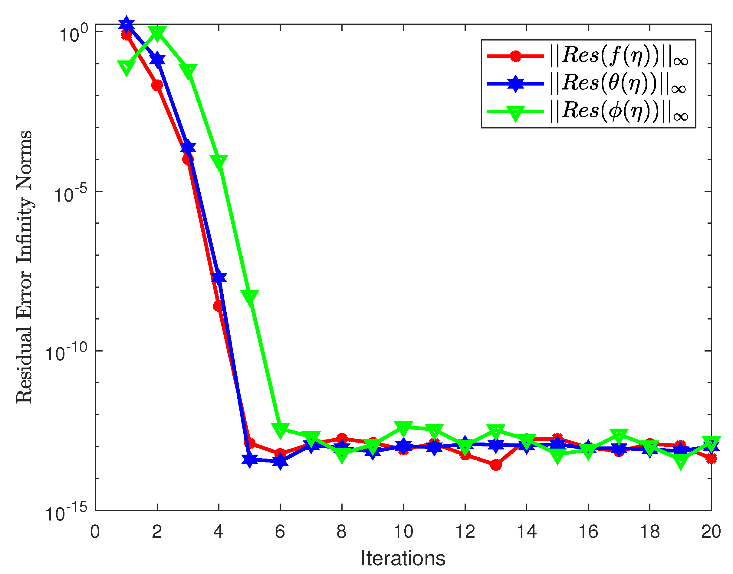
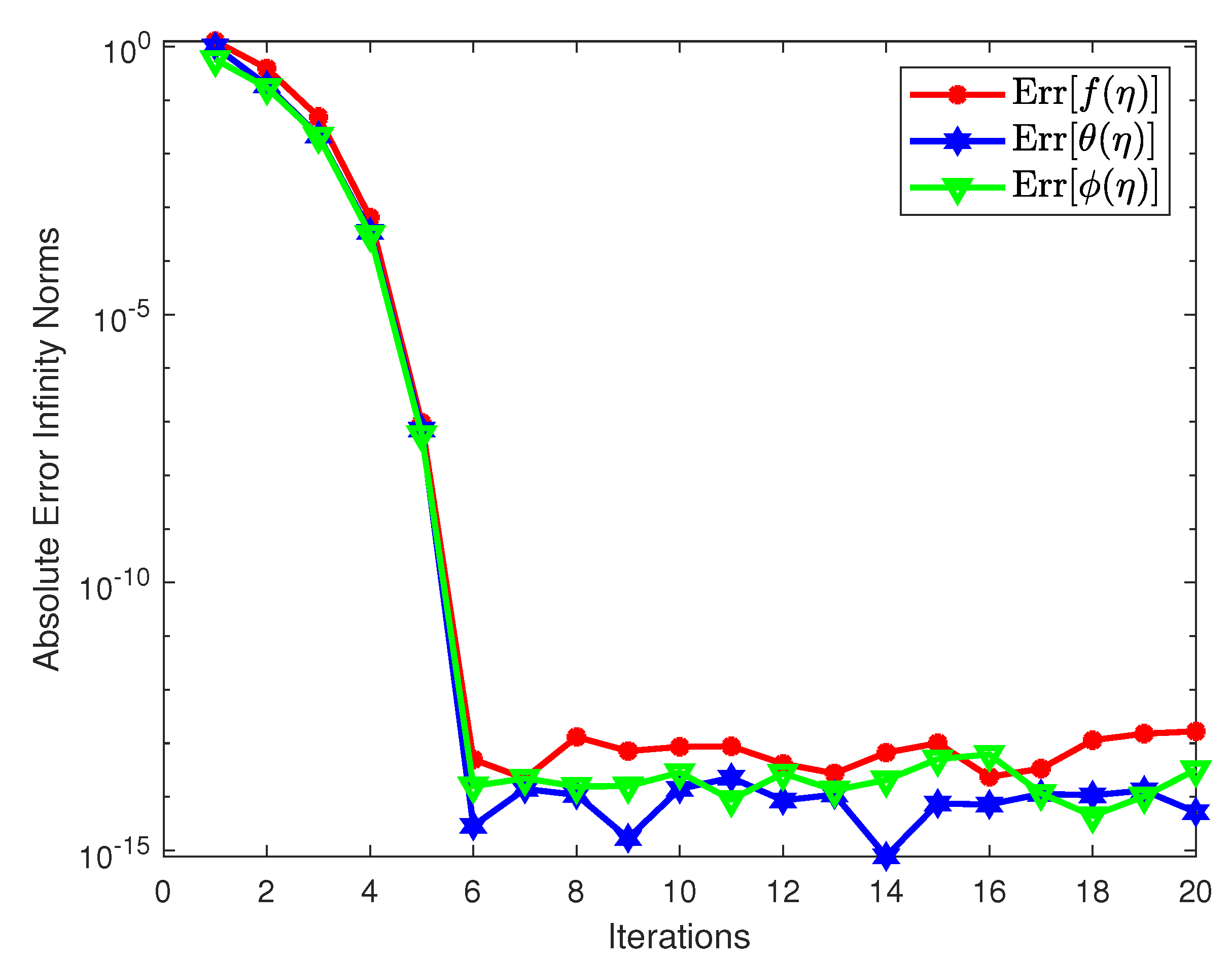
3. Numerical Solution Using the Spectral Quasi-Linearization Method

The system of Equations (9)–(11) subject to boundary conditions Equation (12) are solved using the Spectral Quasi-Linearization Method. In principle, the SQLM algorithm combines two main approaches namely: Quasi-linearization (QLM) and Chebyshev spectral collocation method. The QLM prescription which is used to solve non-linear boundary value problems was originally introduced by Bellman and Kalaba [34] as a generalization of the Newton–Raphson method. In deriving the QLM formula, it is assumed that the solutions of Equations (9)–(11) (and all their derivatives) at the current and previous iterations denoted by $f_r$, ${\theta }_r$,${\varphi }_r$ and $f_{r+1}$, ${\theta }_{r+1}$, ${\varphi }_{r+1}$ respectively, are sufficiently close enough so that multi-variable linear Taylor series yields the following iterative sequence of linear differential equations:

$$a_{0,r}{f}_{r+1}^{‴}+a_{1,r}{f}_{r+1}^{″}+a_{2,r}{f}_{r+1}^{\prime }+a_{3,r}{f}_{r+1}+a_{4,r}{\theta }_{r+1}+a_{5,r}{\varphi }_{r+1}=R_{1,r},$$

(13)

$$b_{0,r}{\theta }_{r+1}^{″}+b_{1,r}{\theta }_{r+1}^{\prime }+b_{2,r}{\theta }_{r+1}+b_{3,r}{f}_{r+1}^{″}+b_{4,r}{f}_{r+1}^{\prime }+b_{5,r}{\varphi }_{r+1}^{\prime }=R_{2,r},$$

(14)

$$c_{0,r}{\varphi }_{r+1}^{″}+c_{1,r}{\varphi }_{r+1}^{\prime }+c_{2,r}{\varphi }_{r+1}+c_{3,r}{f}_{r+1}+c_{4,r}{\theta }_{r+1}^{″}=R_{3,r},$$

(15)

where the variable coefficients evaluated at the current iteration level are defined as:

$$a_{0,r}=1-\beta f_r^2,a_{1,r}=f_r+2\beta f_r{f}_r^{\prime }-A\frac{\eta }{2},a_{2,r}=2\beta f_r{f}_r^{″}-2f_r^{\prime }-A-M,a_{3,r}=f_r^{″}+2\beta f_r^{\prime }{f}_r^{″}-2\beta f_r{f}_r^{‴},$$

$$a_{4,r}=\epsilon ,a_{5,r}=\epsilon N,b_{0,r}=1+\frac{4}{3}R,b_{1,r}=-Pr\left(Nb{\varphi }_r^{\prime }-2Nt{\theta }_r^{\prime }-\frac{\eta }{2}A\right),b_{2,r}=-\frac{3PrA}{2},$$

$$b_{3,r}=2PrEcf{r}^{″},b_{4,r}=2PrEcMf{r}^{\prime },b_{5,r}={\theta }_r^{\prime },b_{6,r}=-PrNb{\theta }_r^{\prime },c_{0,r}=1,c_{1,r}=Sc{f}_r-\frac{ScA\eta }{2},$$

$$c_{3,r}=-\gamma Sc-\frac{ScA}{2},c_{4,r}=Sc{\varphi }_r^{\prime },c_{5,r}=\frac{Nt}{Nb},R_{1,r}=f_r{f}_r^{″}-{\left(f_r\right)}^2+4\beta f_r{f}_r^{\prime }{f}_r^{″}-2\beta {\left(f_r\right)}^2{f}_r^{‴},$$

$$R_{2,r}=PrEc({(f_r^{″})}^2+M{\left(f_r^{\prime }\right)}^2-Nb{\theta }_r^{\prime }{\varphi }_r^{\prime }-Nt{\left({\theta }_r^{\prime }\right)}^2+f_r{\theta }_r^{\prime }),R_{3,r}=Sc{f}_r{\varphi }_r^{\prime }.$$

Additionally, the boundary conditions given in Equation (12) at the current iteration level are:

$$\begin{array}{c}{f}_{r+1}^{\prime }\left(0\right)=1,f_{r+1}\left(0\right)=S,{\theta }_{r+1}\left(0\right)=1,Nb{\varphi }_{r+1}^{\prime }\left(0\right)+Nt{\theta }_{r+1}^{\prime }\left(0\right)=0,\hfill \\ f_{r+1}^{\prime }(\infty )=0,{\theta }_{r+1}(\infty )=0,{\varphi }_{r+1}(\infty )=0.\hfill \end{array}$$

(16)

To apply the Chebyshev pseudo-spectral method, the physical domain $[0,\infty )$ on which Equations (9)–(11) are defined is moved to the computational domain $[-1,1]$ using a linear transformation $\zeta =\frac{2}{L_{\infty }}\eta -1$. The number $L_{\infty }$ is a finite number chosen in such a way that the behaviour of flow properties far away from the sheet are represented. The derivatives of the unknown variables evaluated at Gauss–Lobatto collocation points ${\zeta }_j=cos\left(\frac{\pi j}{N}\right)$,$j=0,1,\cdots ,N$ are approximated by the $(N+1)\times (N+1)$ Chebyshev differentiation matrix $\mathbf{D}=\frac{2}{L_{\infty }}D$, Trefethen [35]. This far, the system of Equations (9)–(11) can written as a vector matrix:

$$\left[\begin{array}{ccc}{\mathbf{a}}_{0,r}{\mathbf{D}}^3+{\mathbf{a}}_{1,r}{\mathbf{D}}^2+{\mathbf{a}}_{2,r}\mathbf{D}+{\mathbf{a}}_{3,r}& a_{4,r}\mathbf{I}& a_{5,r}\mathbf{I}\\ {\mathbf{b}}_{3,r}{\mathbf{D}}^2+{\mathbf{b}}_{4,r}\mathbf{D}& b_{0,r}{\mathbf{D}}^2+{\mathbf{b}}_{1,r}\mathbf{D}+b_{2,r}{\mathbf{D}}^2& b_{5,r}\mathbf{D}\\ {\mathbf{c}}_{3,r}& c_{4,r}{\mathbf{D}}^2& c_{0,r}{\mathbf{D}}^2+{\mathbf{c}}_{1,r}\mathbf{D}+c_{2,r}\mathbf{I}\end{array}\right]\left[\begin{array}{c}{\mathbf{F}}_{r+1}\\ {\mathbf{\Theta }}_{r+1}\\ {\mathbf{\Phi }}_{r+1}\end{array}\right]=\left[\begin{array}{c}{\mathbf{R}}_{1,r}\\ {\mathbf{R}}_{2,r}\\ {\mathbf{R}}_{3,r}\end{array}\right],$$

(17)

subject to boundary conditions

$$\begin{array}{c}{\mathbf{F}}_{r+1}^{\prime }\left({\eta }_N\right)=1,{\mathbf{F}}_{r+1}\left({\eta }_N\right)=S,{\mathrm{\Theta }}_{r+1}\left({\eta }_n\right)=1,Nb{\mathrm{\Phi }}_{r+1}^{\prime }\left({\eta }_N\right)+Nt{\mathbf{\Theta }}_{r+1}^{\prime }\left({\eta }_N\right)=0,\hfill \\ {\mathbf{F}}_{r+1}^{\prime }\left({\eta }_0\right)=0,{\mathbf{\Theta }}_{r+1}\left({\eta }_0\right)=0,{\mathbf{\Phi }}_{r+1}\left({\eta }_0\right)=0,\hfill \end{array}$$

(18)

where

$$\begin{array}{ccc}& & {\mathbf{F}}_{r+1}={[f_{r+1}\left({\eta }_0\right),f_{r+1}\left({\eta }_1\right),\cdots ,f_{r+1}\left({\eta }_{N-1}\right),f_{r+1}\left({\eta }_N\right)]}^T,\hfill \\ & & {\mathbf{\Theta }}_{r+1}={[{\theta }_{r+1}\left({\eta }_0\right),{\theta }_{r+1}\left({\eta }_1\right),\cdots ,{\theta }_{r+1}\left({\eta }_{N-1}\right),{\theta }_{r+1}\left({\eta }_N\right)]}^T,\hfill \\ & & {\mathrm{\Phi }}_{r+1}={[{\varphi }_{r+1}\left({\eta }_0\right),{\varphi }_{r+1}\left({\eta }_1\right),\cdots ,{\varphi }_{r+1}\left({\eta }_{N-1}\right),{\varphi }_{r+1}\left({\eta }_N\right)]}^T,\hfill \\ & & {\mathbf{a}}_{q,r}=\left(\begin{array}{cccccc}{a}_{q,r}\left({\eta }_0\right)& & & & & \\ & a_{q,r}\left({\eta }_1\right)& & & & \\ & & \ddots & & \\ & & & a_{q,r}\left({\eta }_{N-1}\right)& \\ & & & & & a_{q,r}\left({\eta }_N\right)\end{array}\right),q=0,1,\cdots ,5.\hfill \end{array}$$

Diagonal matrices ${\mathbf{b}}_{q,r},(q=0,1,\cdots ,5)$ and ${\mathbf{c}}_{q,r},(q=0,1,\cdots ,4)$ have the same definition as the diagonal matrix ${\mathbf{a}}_{q,r}$ and $\mathbf{I}$ is an $(N+1)\times (N+1)$ identity matrix.

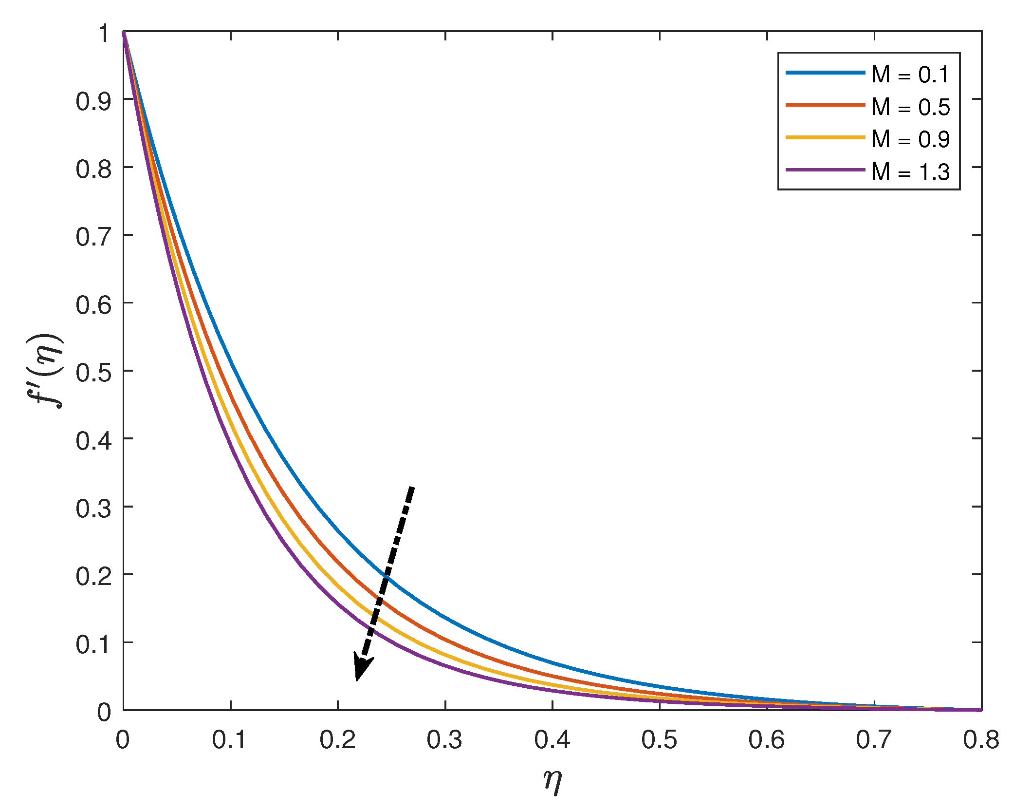
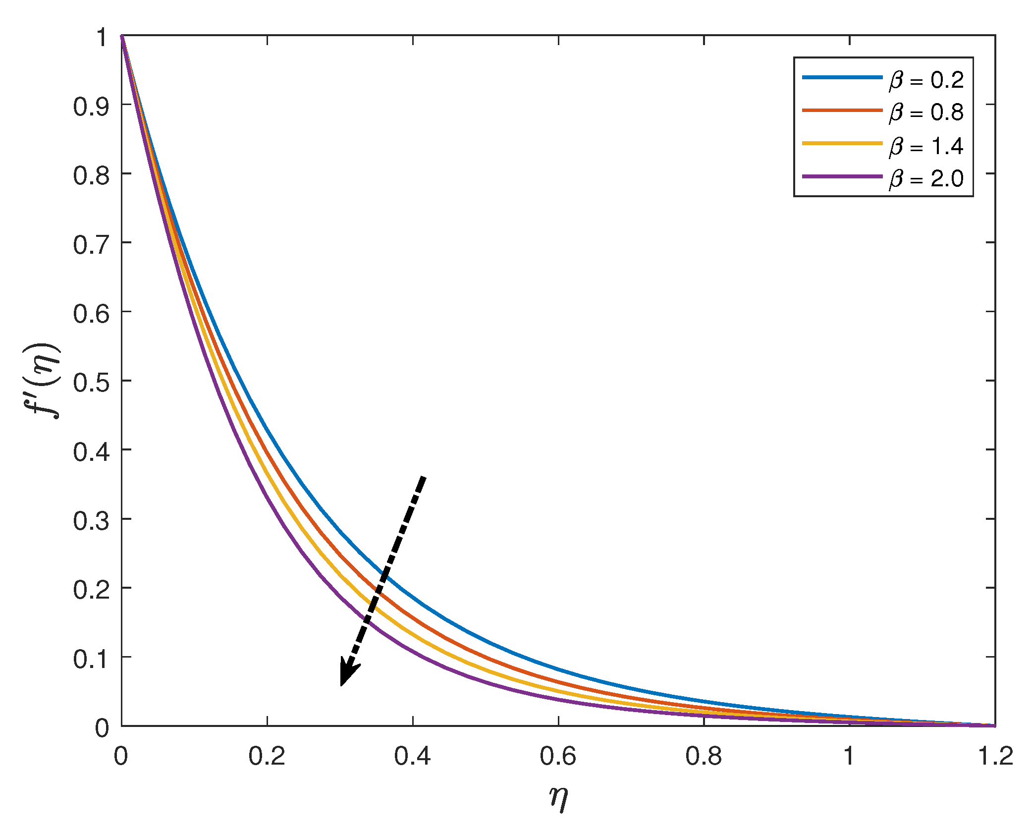
4. Results and Discussions

The system of equations in vector matrix form Equation (17) together with boundary conditions in Equation (18) is solved using the Spectral quasi-linearization method implemented on MATLAB R2020a. To ascertain the accuracy and the convergence of the numerical technique used, solution based error infinity norms were used. The default values of the parameters (unless otherwise stated) used to achieve the desired accuracy, convergence and for all the numerical simulations in this study are: $N=60$, $L_{\infty }=0.8$, $A=0.4$, $\beta =0.1$, $ϵ=0.1$, $M=1.0$, $Pr=0.71$, $R_d=0.1$, $Ec=0.1$, $Nb=0.3$, $Nt=0.3$, $Sc=0.6$ and $\gamma =1.0$. Figure 2 is plotted to reveal the relationship between the residual error infinity norms and increased iterations. The residual error approximates the true solution to about ${10}^{-14}$ after six iterations. This confirms that the SQLM algorithm is very accurate. Figure 3 portrays that the solution based errors defined as:

$$\mathrm{E}\mathrm{r}\mathrm{r}\left[f\left(\eta \right)\right]=\left|\right|{\mathbf{F}}_{r+1}-{\mathbf{F}}_r{\left|\right|}_{\infty },\mathrm{E}\mathrm{r}\mathrm{r}\left[\mathrm{\Theta }\left(\eta \right)\right]=\left|\right|{\mathbf{\Theta }}_{r+1}-{\mathbf{\Theta }}_r{\left|\right|}_{\infty },\mathrm{E}\mathrm{r}\mathrm{r}\left[\mathrm{\Phi }\left(\eta \right)\right]=\left|\right|{\mathbf{\Phi }}_{r+1}-{\mathbf{\Phi }}_r{\left|\right|}_{\infty },$$

diminish as the number of iteration is increased. This proves that the method is convergent.

To validate the SQLM results obtained in this study,

Table 1. The values of $-f^{″}\left(0\right)$ compared with published results for selected values of $\mathit{A}$.

A	Elbashbeshy and Bzid [36]	Hussain et al. [18]	Present Study
0.8	1.3321	1.3333	1.331497109737629
1.2	1.4691	1.4684	1.469781692104270
2.0	1.7087	1.7090	1.713344535151333

displays the values of the skin friction coefficient $(-f^{″}\left(0\right))$ when $\beta =M=ϵ=0$ for different values of the unsteadiness parameter $\left(A\right)$ compared against the results obtained earlier by Hussain et al. [18] and Elbashbeshy and Bazid [36]. There is a good agreement of the results obtained in the present study with those in the mentioned published literature.

Table 2. The values of $-f^{″}\left(0\right)$ and $-(1+\frac{4}{3}{R}_d){\theta }^{\prime }(0)$ compared with published results and Matlab bvp4c for selected values of M and S when $A=0=\beta$, $M=1.0=\gamma$, $Nt=Nb=Ec=R_d=0.1$, $Sc=0.6$ and $Pr=0.71$.

M	S	$-{\mathit{f}}^{″}\left(0\right)$			$-\left(1+\frac{4}{3}{\mathit{R}}_{\mathit{d}}\right){\mathit{\theta }}^{\prime }\left(0\right)$
		Ibrahim and Shankar [37]	Matlab Bvp4c	SQLM	Matlab Bvp4c	SQLM
0	0.5	1.2808	1.28077620	1.28077641	0.60136784	0.60136784
0.5		1.5000	1.50000000	1.50000000	0.55812915	0.55813015
1.0		1.6861	1.68614066	1.68614066	0.52446025	0.52446152
1.5		1.8508	1.85078106	1.85078106	0.49672490	0.49672670
2.0		2.0000	2.00000000	2.00000000	0.47305633	0.47305881
1.0	0	1.4142	1.41421356	1.41421356	0.29167318	0.29167374
	0.2	1.5177	1.51774469	1.51774469	0.38145187	0.38145259
	0.7	1.8069	1.80688023	1.80688023	0.62431224	0.62431389
	1.0	2.0000	2.00000000	2.00000000	0.77943236	0.77942860

depicts the numerical values of $-f^{″}\left(0\right)$ and $-\left(1+\frac{4}{3}{R}_d\right){\theta }^{\prime }\left(0\right)$ when $A=ϵ=0$ and varying the values of the magnetic parameter $\left(M\right)$ and suction-injection parameter $\left(S\right)$. The results obtained are in excellent agreement with those obtained by Ibrahim and Shankar [37] and Matlab bvp4c.

The impact of the magnetic parameter $\left(M\right)$ on the fluid velocity is portrayed in Figure 4. It is noted that an increase in the magnetic parameter significantly reduces the velocity of the nanofluid throughout the boundary layer. Physically, the application of a transverse magnetic field results in a Lorentz force that has a tendency to create a resistance to the fluid flow. Figure 5, Figure 6 and Figure 7 reflect the Maxwell parameter $\left(\beta \right)$, mixed convection parameter $\left(ϵ\right)$ and the unsteadiness parameter $\left(A\right)$ on the velocity profiles. It is apparent in Figure 5 that the velocity profiles of the Maxwell nanofluid decline as $\beta$ is enhanced. Physically, at high values of $\beta$, the fluid demonstrates a solid-like behaviour hence a reduced velocity. It is observed in Figure 6 that the velocity distribution and the momentum boundary layer are enhanced as the values of $ϵ$ are increased. Figure 7 shows that increasing the unsteadiness parameter reduces the velocity profiles and the momentum boundary layer thickness. This shows that the flow rate as a result of the stretching sheet is reduced as the unsteadiness parameter is increased.

Figure 8, Figure 9, Figure 10 and Figure 11 display the impacts of Eckert number $\left(Ec\right)$, thermal radiation parameter $\left(R_d\right)$, Prandtl number $\left(Pr\right)$ and the thermophoresis parameter $\left(Nt\right)$ on the temperature distributions of the Maxwell nanofluid. Figure 8 reflects clearly that increasing the $Ec$ values causes an upsurge in the temperature profiles. The Eckert number, which is used to characterise the impact of self-heating of the Maxwell nanofluid fluid due to dissipation effects, is a dimensionless number that represents the relationship between kinetic energy and enthalpy. The heat energy that is stored in the nanofluid due to frictional heating has the effect of enhancing the temperature of the fluid. It is clearly illustrated in Figure 9 that the fluid temperature is suppressed as the Prandlt number increases. Physically, increasing $Pr$ entails a decrease in the thermal diffusivity that will also cause a decrease of the energy transfer ability. As a result, both the temperature and thermal boundary layer decrease. Figure 10 reveals that the fluid temperature is an increasing function of the thermal radiation parameter. For larger values of $R_d$, more heat is provided to the working fluid which in turn enhances the temperature and the thermal boundary layer thickness. The influence of the thermophoresis parameter is depicted in Figure 11. It is noted that increasing the values of $Nt$ causes a decrease in the fluid temperature profiles.

Figure 12, Figure 13, Figure 14 and Figure 15 present the effects of the chemical reaction parameter $\left(\gamma \right)$, Brownian motion parameter $\left(Nb\right)$, the Schmidt number $\left(Sc\right)$ and the thermophoresis parameter $\left(Nt\right)$ on the nano-particle volume fraction profiles. The influence of the chemical reaction parameter on the concentration distributions of the Maxwell nanofluid is reflected in Figure 12. It is noted that an increase in the destructive chemical reaction parameter decreases the concentration field. Physically, when the chemical reaction parameter is enhanced, more solute molecules will undergo chemical reaction and hence the concentration and solutal boundary layer thickness is reduced. Figure 13 reveals that increasing the $Sc$ values suppresses the concentration profiles. In effect, $Sc$ correlates the momentum transport diffusion in the hydrodynamic boundary layer and the species diffusion in the concentration boundary layer. Larger values of the Schmidt number are equivalent to decreasing chemical molecular diffusivity and vice versa. The concentration boundary layer thickness is reduced with increased values of $Sc$. Figure 14 and Figure 15 highlight the significance of the Brownian motion parameter and the thermophoresis parameter on the concentration fields, respectively. The nano-particle concentration is a decreasing function of $Nb$ whilst the opposite trend is observed for $Nt$. Due to temperature gradient, increasing the values of $Nt$ enhances a thermophoresis force which in turn causes diffusion of the nano-particles in the ambient fluid and hence thickens the concentration boundary layer.

Table 3. Computation of the values of skin friction coefficient $(-f^{″}\left(0\right))$, the local Nusselt number $(-{\theta }^{\prime }\left(0\right))$ and the local Sherwood number $-{\varphi }^{\prime }\left(0\right)$ for different values of $Ec$, $Pr$, $R_d$, $Nb$, $Nt$, $Sc$, $\gamma$ when $ϵ=0.1$, $\beta =0.1$, $M=0.1$, $A=0.4$.

Ec	Pr	${\mathit{R}}_{\mathit{d}}$	Nb	Nt	Sc	$\mathit{\gamma }$	$-{\mathit{f}}^{\prime \prime }\left(0\right)$	$-\left(1+\frac{4}{3}{\mathit{R}}_{\mathit{d}}\right){\mathit{\theta }}^{\prime }\left(0\right)$	$-{\mathit{\varphi }}^{\prime }\left(0\right)$
0.1	0.71	0.1	0.3	0.3	0.6	1.0	1.516610	0.686537	−0.686537
0.3							1.515505	0.574942	−0.574942
0.5							1.514401	0.463533	−0.463533
	1.0						1.519931	0.819431	−0.819431
	2.0						1.526872	1.171820	−1.171820
	3.0						1.530777	1.439856	−1.439856
		1.0					1.510498	0.479179	−0.479179
		1.5					1.508763	0.426789	−0.426789
		2.0					1.507540	0.391166	−0.391166
			0.5				1.516226	0.686539	−0.411924
			0.7				1.516061	0.686540	−0.294231
			0.9				1.515969	0.686540	−0.228846
				0.5			1.517497	0.695090	−1.158483
				0.7			1.518385	0.703747	−1.642076
				0.9			1.519272	0.712507	−2.137521
					0.8		1.516506	0.688506	−0.688506
					1.0		1.516438	0.690138	−0.690138
					1.2		1.516391	0.691529	−0.691528
						2.0	1.516512	0.690097	−0.690097
						3.0	1.516449	0.692653	−0.692653
						4.0	1.516405	0.694631	−0.694631

displays the values the skin friction coefficient $(-f^{″}\left(0\right))$, the local Nusselt number $(-{\theta }^{\prime }\left(0\right))$ and the local Sherwood number $(-{\varphi }^{\prime }\left(0\right))$ for different values of the Eckert number, Prandtl number, thermal radiation parameter, Brownian motion parameter, thermophoresis parameter, Schmidt number and the chemical reaction parameter. It is noted that the $-f^{″}\left(0\right)$ is enhanced when the values of $Pr$ and $Nt$ are increased and is suppressed with increased value of $Ec$, $R_d$, $Nb$, $Sc$ and $\gamma$. The local Nusselt number is an increasing function of $Pr$, $Nt$, $Sc$, and $\gamma$ whilst it decreases when the values of $Ec$, $R_d$ and $Nb$ are increased. It is observed that there is an upsurge in the local Sherwood number with increasing $Pr$, $Nt$, $Sc$ and $\gamma$ whilst an opposite trend is realised when $Ec$, $R_d$ and $Nb$ are increased.

5. Conclusions

An investigation of the flow of a thermomagnetic Maxwell nanofluid flowing past a stretching or shrinking plate in the presence of Ohmic dissipation and Brownian motion was carried out. The governing non-linear partial differential equations were reduced to non-linear ordinary differential equations which were then solved using the Spectral Quasi-Linearization Method. Solution based errors showed that the numerical technique used is very accurate and converges after a few iterations. Results obtained in this study were found to be in agreement with those existing in the literature. The impact of some chosen important physical parameters on the velocity, temperature and concentration boundary layers of the Maxwell nanofluid were discussed in detail. Core points from the study are:

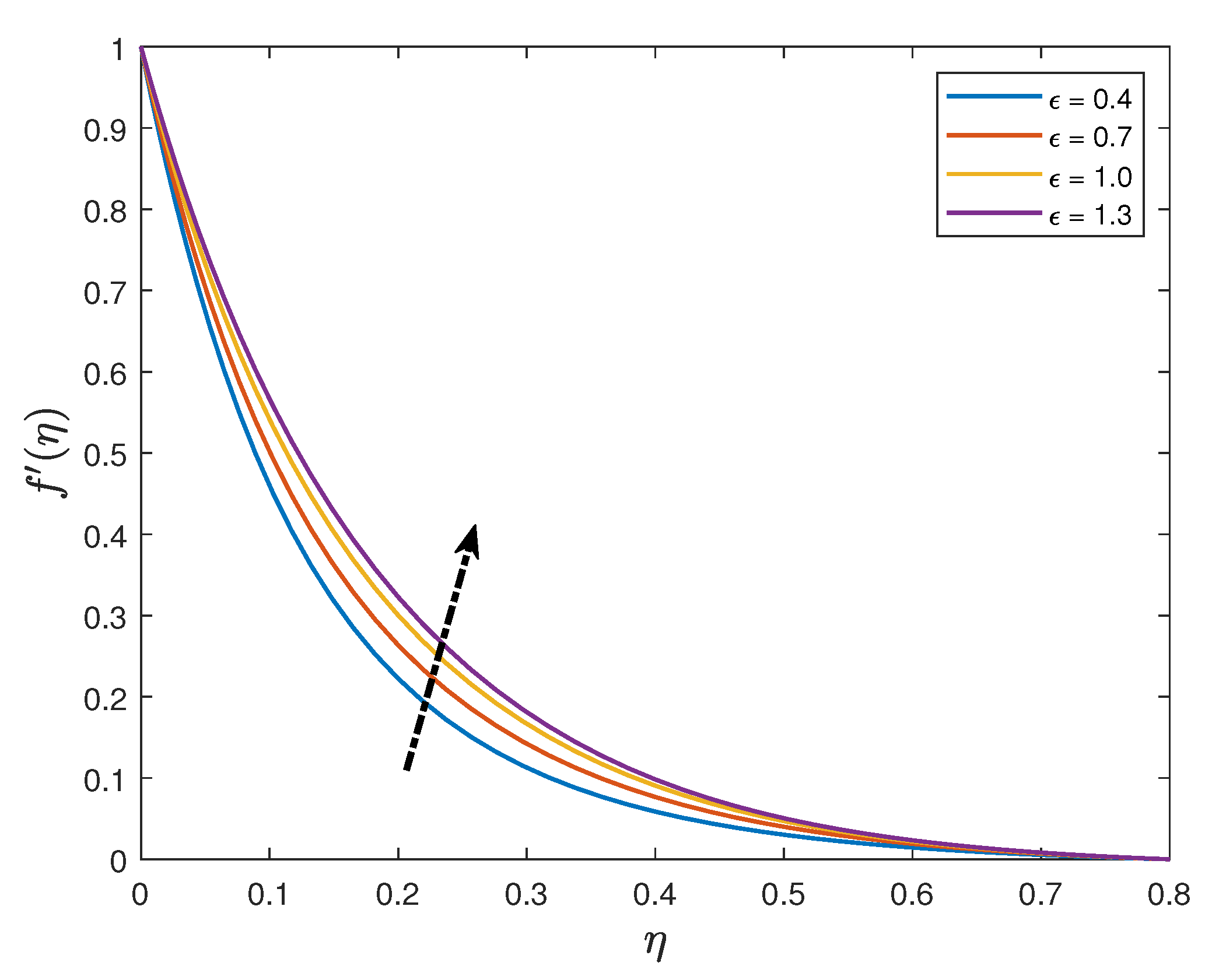
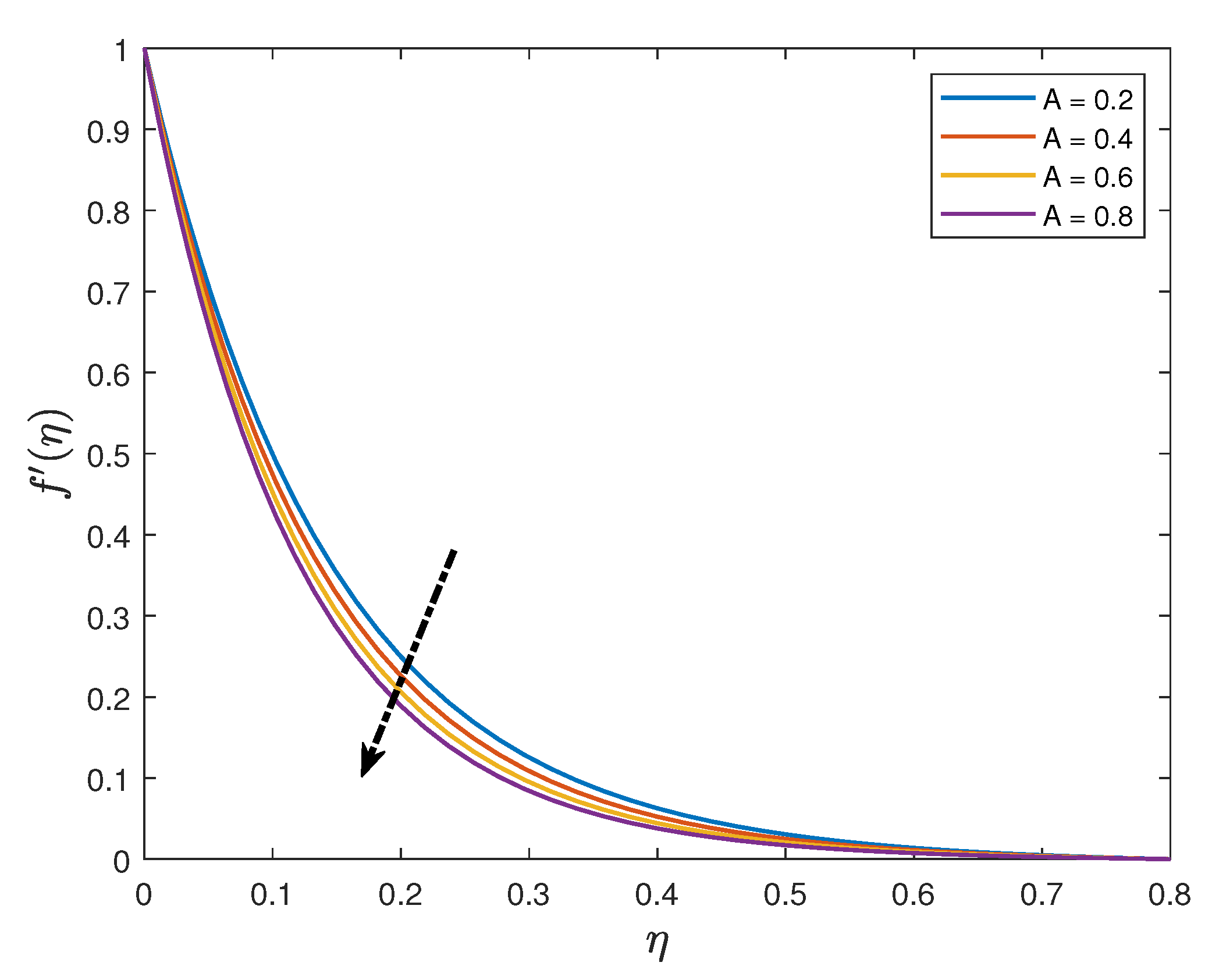
• The velocity distribution increases with an enhancement of the mixed convection parameter whilst it reduces when the values of the magnetic parameter, unsteadiness parameter and the Maxwell parameter are increased;
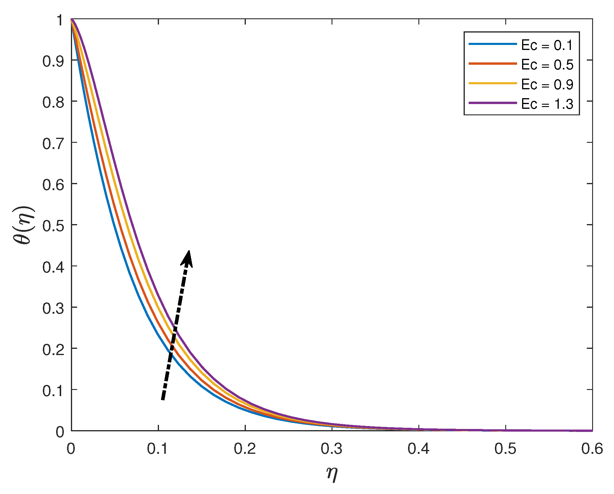
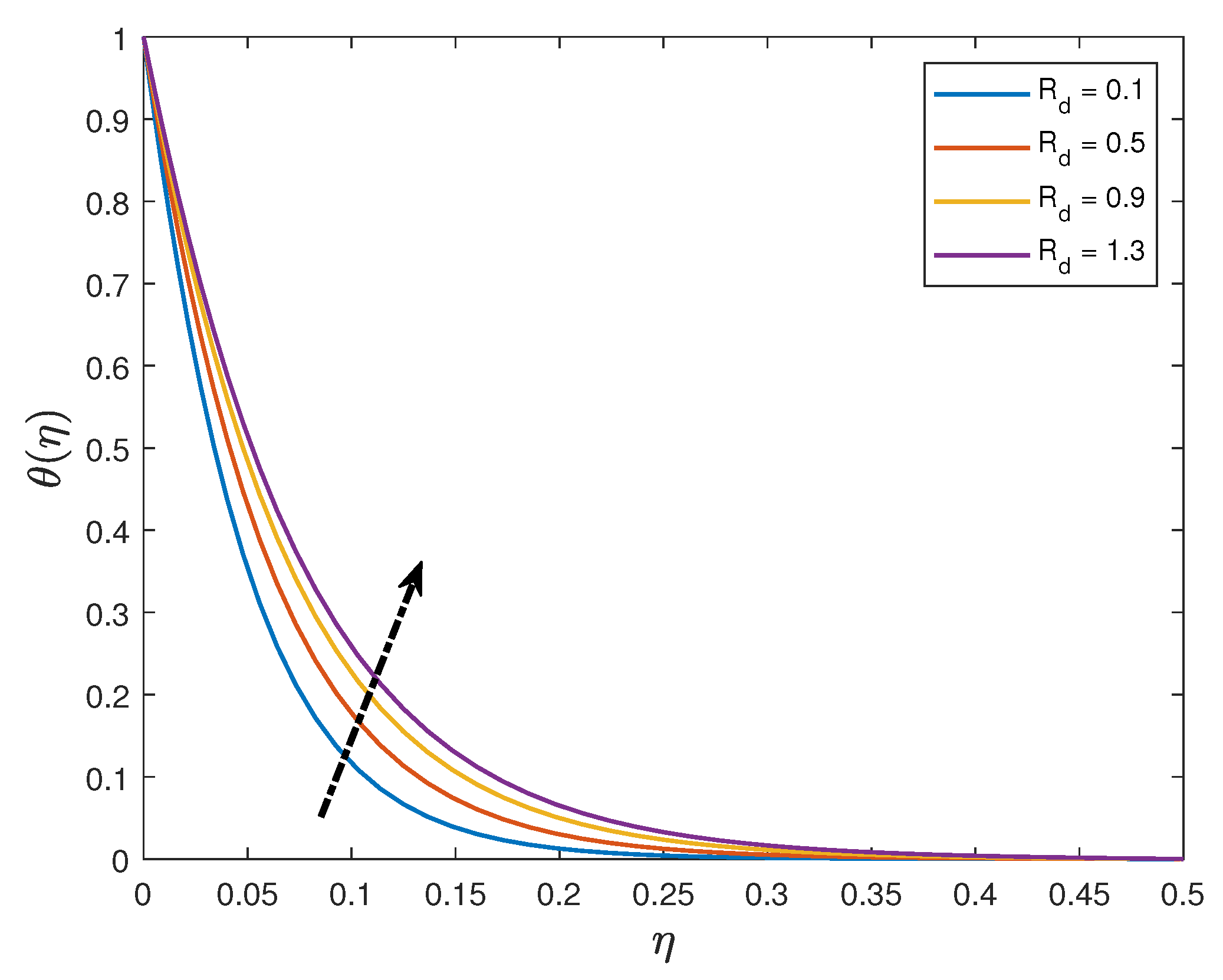
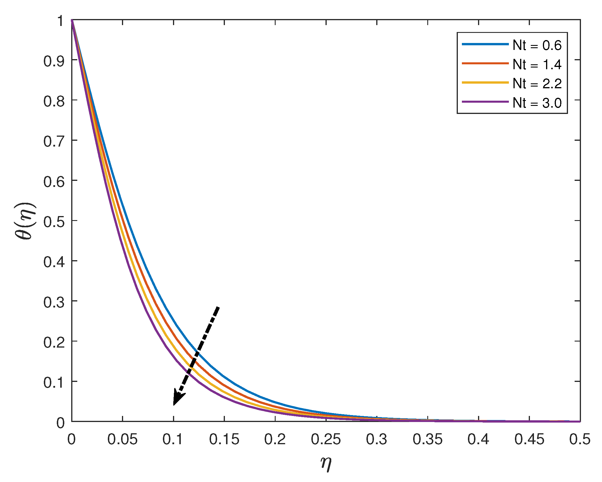
• Increasing the values of the Eckert number and thermal radiation parameter enhances the temperature profiles whilst the profiles are depressed when the Prandtl number and the thermophoresis parameter are increased;
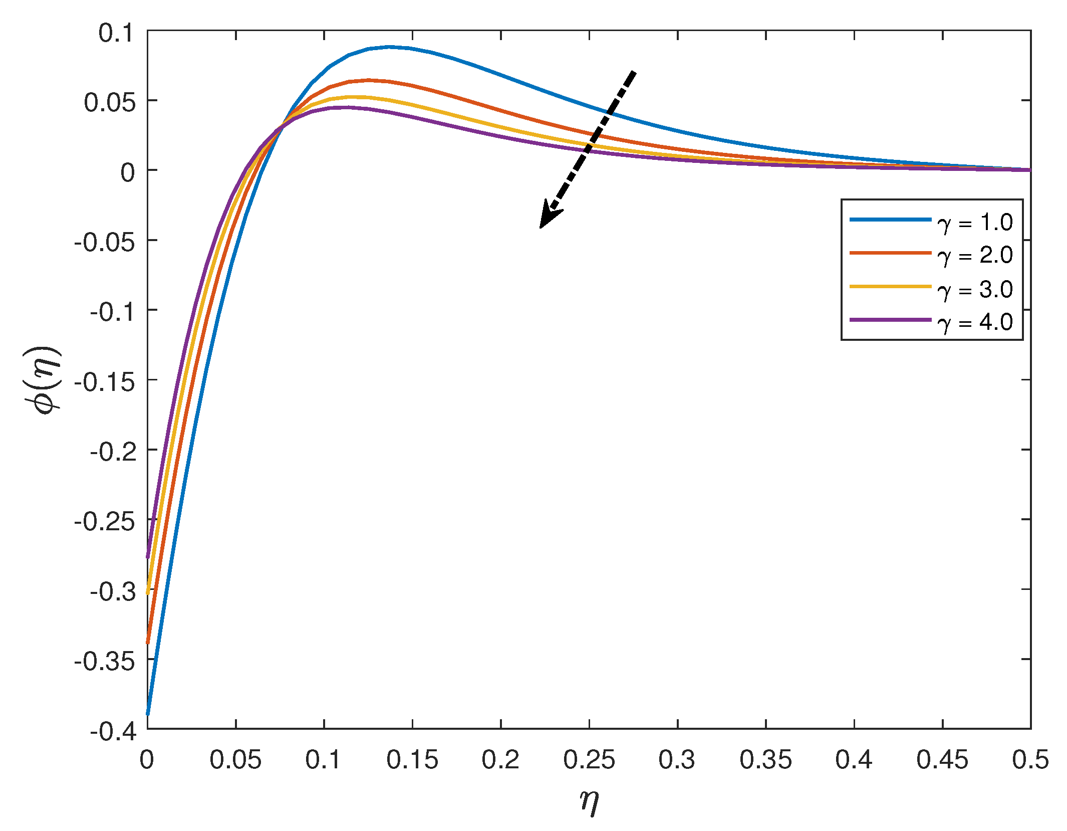
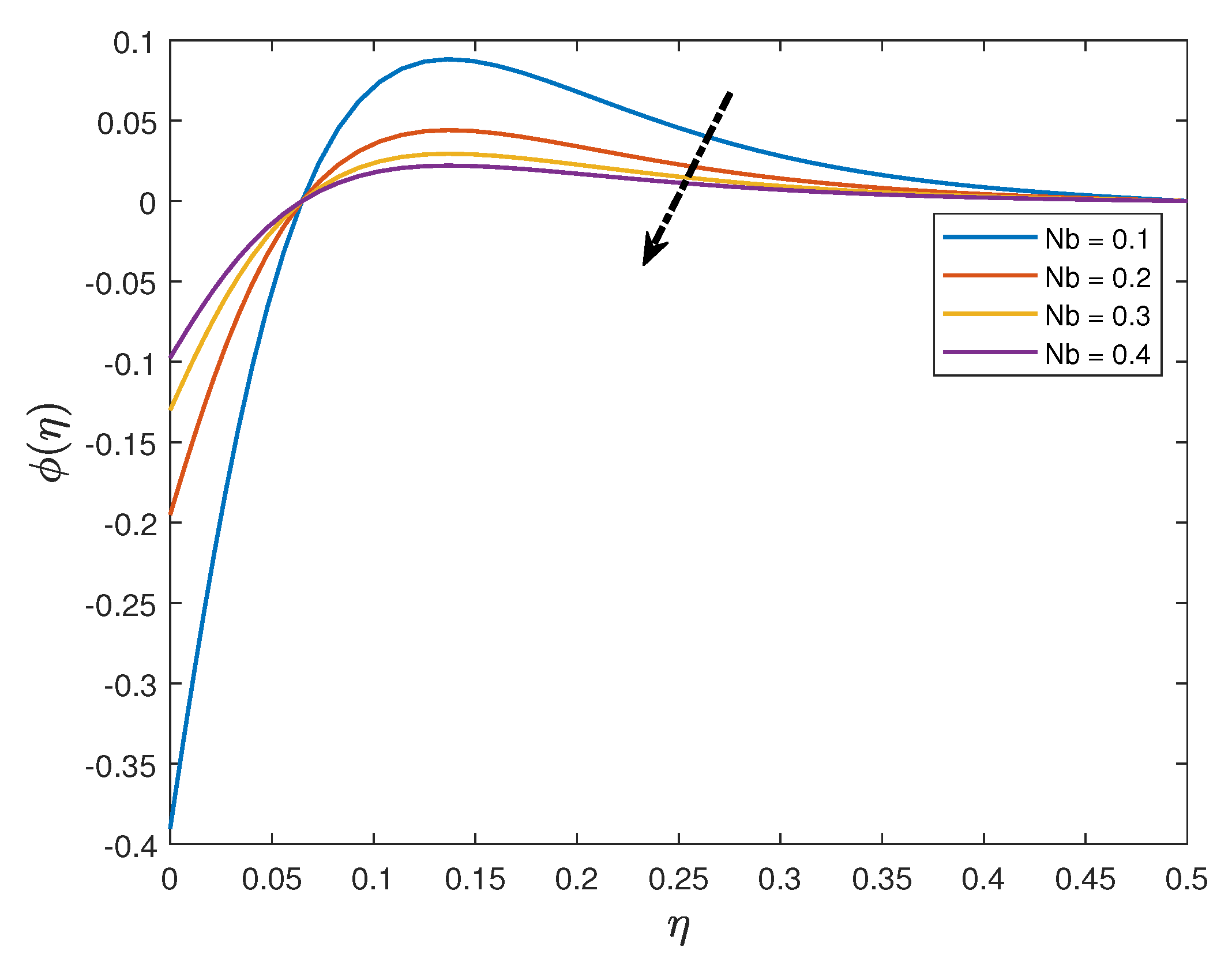
• The nanoparticle concentration distribution is an increasing function of the thermophoresis parameter and a decreasing function of thermal radiation parameter, Schmidt number and the Brownian motion parameter.

References

1. Choi, S.U.S.; Eastman, J.A. Enhancing Thermal Conductivity of Fluids with Nanoparticles; Argonne National Laboratory (ANL): Argonne, IL, USA, 1995.
2. Jakati, S.V.; Raju, T.B.; Nargund, A.L.; Sathyanarayana, S.B. Study of Maxwell Nanofluid Flow over a Stretching Sheet with Non-Uniform Heat Source/Sink with External Magnetic Field. J. Adv. Res. Fluid Mech. Therm. Sci. 2021, 55, 218–232. [Google Scholar]
3. Hayat, T.; Qayyum, S.; Alsaedi, A. Mechanisms of nonlinear convective flow of Jeffrey nanofluid due to nonlinear radially stretching sheet with convective conditions and magnetic field. Results Phys. 2017, 7, 2341–2351. [Google Scholar] [CrossRef]
4. Maxwell, J.C. On the Dynamical Theory of Gases. Philos. Trans. R. Soc. Lond. 1867, 157, 49–88. [Google Scholar] [CrossRef]
5. Ellahi, R.; Raza, M.; Vafai, K. Series solutions of non-Newtonian nanofluids with Reynolds’ model and Vogel’s model by means of the homotopy analysis method. Math. Comput. Model. 2012, 55, 1876–1891. [Google Scholar] [CrossRef]
6. Crane, L.J. Flow past a stretching plate. Z. Angew. Math. Phys. 1970, 21, 645–647. [Google Scholar] [CrossRef]
7. Khan, S.; Selim, M.M.; Khan, A.; Ullah, A.; Abdeljawad, T.; Ikramullah; Ayaz, M.; Mashwani, W.K. On the Analysis of the Non-Newtonian Fluid Flow Past a Stretching/Shrinking Permeable Surface with Heat and Mass Transfer. Coatings 2021, 11, 566. [Google Scholar] [CrossRef]
8. Kudenatti; Ramesh, B.; Misbah, N.-E. Hydrodynamic flow of non-Newtonian power-law fluid past a moving wedge or a stretching sheet: A unified computational approach. Sci. Rep. 2020, 101, 9445. [Google Scholar] [CrossRef]
9. Gireesha, B.J.; Umeshaiah, M.; Prasannakumara, B.C.; Shashikumar, N.S.; Archana, M. Impact of nonlinear thermal radiation on magnetohydrodynamic three dimensional boundary layer flow of Jeffrey nanofluid over a nonlinearly permeable stretching sheet. Phys. A Stat. Mech. Appl. 2020, 549, 124051. [Google Scholar] [CrossRef]
10. Shahzad, F.; Jamshed, W.; Nisar, K.S.; Nasir, N.A.A.M. Thermal analysis for Al2O3–sodium alginate magnetized Jeffrey’s nanofluid flow past a stretching sheet embedded in a porous medium. Sci. Rep. 2022, 12, 3287. [Google Scholar] [CrossRef]
11. Jayachandra Babu, M.; Sandeep, N. MHD non-Newtonian fluid flow over a slendering stretching sheet in the presence of cross-diffusion effects. Alex. Eng. J. 2016, 55, 2193–2201. [Google Scholar] [CrossRef]
12. Baranovskii, E.S. Flows of a polymer fluid in domain with impermeable boundaries. Comput. Math. Math. Phys. 2014, 54, 1589–1596. [Google Scholar] [CrossRef]
13. Ibrahim, S.M.; Kumar, P.V.; Makinde, O.D. Chemical Reaction and Radiation Effects on Non-Newtonian Fluid Flow over a Stretching Sheet with Non-Uniform Thickness and Heat Source. Defect Diffus. Forum 2018, 387, 319–331. [Google Scholar] [CrossRef]
14. Khan, W.; Idress, M.; Gul, T.; Khan, M.A.; Bonyah, E. Three non-Newtonian fluids flow considering thin film over an unsteady stretching surface with variable fluid properties. Adv. Mech. Eng. 2018, 10, 1687814018807361. [Google Scholar] [CrossRef]
15. Sahoo, B. Flow and heat transfer of a non-Newtonian fluid past a stretching sheet with partial slip. Commun. Nonlinear Sci. Numer. Simul. 2010, 15, 602–615. [Google Scholar] [CrossRef]
16. Mishra, S.R.; Baag, S.; Dash, G.C.; Acharya, M.R. Numerical approach to MHD flow of power-law fluid on a stretching sheet with non-uniform heat source. Nonlinear Eng. 2019, 9, 81–93. [Google Scholar] [CrossRef]
17. Prasannakumara, B.C. Numerical simulation of heat transport in Maxwell nanofluid flow over stretching sheet considering magnetic dipole effect. Partial Differ. Equ. Appl. Math. 2021, 4, 100064. [Google Scholar] [CrossRef]
18. Hussain, S.M.; Sharma, R.; Mishra, M.R.; Alrashidy, S.S. Hydromagnetic Dissipative and Radiative Graphene Maxwell Nanofluid Flow Past a Stretched Sheet-Numerical and Statistical Analysis. Mathematics 2020, 8, 1929. [Google Scholar] [CrossRef]
19. Ibrahim, W.; Negera, M. MHD slip flow of upper-convected Maxwell nanofluid over a stretching sheet with chemical reaction. J. Egypt. Math. Soc. 2020, 28, 7. [Google Scholar] [CrossRef]
20. Ahmad, S.; Khan, M.N.; Nadeem, S. Unsteady three dimensional bioconvective flow of Maxwell nanofluid over an exponentially stretching sheet with variable thermal conductivity and chemical reaction. Int. J. Ambient Energy 2022. [Google Scholar] [CrossRef]
21. Jawad, M.; Saeed, A.; Gul, T.; Shah, Z.; Kumam, P. Unsteady thermal Maxwell power law nanofluid flow subject to forced thermal Marangoni Convection. Sci. Rep. 2021, 11, 7521. [Google Scholar] [CrossRef]
22. Motsa, S.S.; Dlamini, P.G.; Khumalo, M. Spectral Relaxation Method and Spectral Quasilinearization Method for Solving Unsteady Boundary Layer Flow Problems. Adv. Math. Phys. 2014, 2014, 341964. [Google Scholar] [CrossRef]
23. Rai, N.; Mondal, S. Spectral methods to solve nonlinear problems: A review. Partial Differ. Equ. Appl. Math. 2021, 4, 100043. [Google Scholar] [CrossRef]
24. Alharbey, R.A.; Mondal, H.; Behl, R. Spectral Quasi-Linearization Method for Non-Darcy Porous Medium with Convective Boundary Condition. Entropy 2019, 21, 838. [Google Scholar] [CrossRef]
25. Magodora, M.; Mondal, H.; Sibanda, P. Effect of Cattaneo-Christov Heat Flux on Radiative Hydromagnetic Nanofluid Flow between Parallel Plates using the Spectral Quasilinearization Method. J. Appl. Comput. Mech. 2022, 8, 865–875. [Google Scholar] [CrossRef]
26. Mondal, H.; Sibanda, P. Spectral Quasi-Linearization Method for Entropy Generation Using the Cattaneo–Christov Heat Flux Model. Int. J. Comput. Methods 2018, 17, 1940002. [Google Scholar] [CrossRef]
27. Mondal, H.; Bharti, S. Spectral Quasi-linearization for MHD Nanofluid Stagnation Boundary Layer Flow due to a Stretching/Shrinking Surface. J. Appl. Comput. Mech. 2020, 6, 1058–1068. [Google Scholar] [CrossRef]
28. Nayak, R.E.; Rao, M.V.S.; Gangadhar, K. Mixed convection boundary layer flow of non-Newtonian nanofluid using the spectral quasi linearization. Math. Model. Eng. Probl. 2020, 7, 45–54. [Google Scholar] [CrossRef]
29. Sahoo, A.; Nandkeolyar, R. Entropy generation and dissipative heat transfer analysis of mixed convective hydromagnetic flow of a Casson nanofluid with thermal radiation and Hall current. Sci. Rep. 2021, 11, 3926. [Google Scholar] [CrossRef]
30. Kierzenka, J.; Shampine, L.F. A BVP solver based on residual control and the MATLAB PSE. ACM Trans. Math. Soft. 2001, 27, 299–316. [Google Scholar] [CrossRef]
31. Madhu, M.; Kishan, N.; Chamkha, A.J. Unsteady flow of a Maxwell nanofluid over a stretching surface in the presence of magnetohydrodynamic and thermal radiation effects. Propuls. Power Res. 2017, 6, 31–40. [Google Scholar] [CrossRef]
32. El-Aziz, M.A.; Yahya, A.S. Heat and Mass Transfer of Unsteady Hydromagnetic Free Convection Flow Through Porous Medium Past a Vertical Plate with Uniform Surface Heat Flux. J. Theor. Appl. Mech. 2017, 47, 25–58. [Google Scholar] [CrossRef]
33. Daniel, Y.S.; Aziz, Z.A.; Ismail, Z.; Salah, F. Thermal radiation on unsteady electrical MHD flow of nanofluid over stretching sheet with chemical reaction. J. King Saud Univ.—Sci. 2017, 31, 804–812. [Google Scholar] [CrossRef]
34. Bellman, R.; Kalaba, R. Quasilinearization and Nonlinear Boundary-Value Problems; American Elsevier Publishing Company: New York, NY, USA, 1965. [Google Scholar]
35. Trefethen, L.N. Spectral Methods in MATLAB; Society for Industrial and Applied Mathematics: Philadelphia, PA, USA, 2000. [Google Scholar]
36. Elbashbeshy, E.M.A.; Bazid, M.A.A. Heat transfer over an unsteady stretching surface. Heat Mass Transfer 2004, 41, 1–4. [Google Scholar] [CrossRef]
37. Ibrahim, W.; Shankar, B. MHD boundary layer flow and heat transfer of a nanofluid past a permeable stretching sheet with velocity, thermal and solutal slip boundary conditions. Comput. Fluids 2013, 75, 1–10. [Google Scholar] [CrossRef]
Figure 1. Schematic flow diagram and coordinate system.
Fluids 07 00252 g001
Figure 2. Accuracy graphs of f, θ and ϕ .
Fluids 07 00252 g002
Figure 3. Convergence graphs of f, θ and ϕ .
Fluids 07 00252 g003
Figure 4. Influence of M on the nanofluid velocity.
Fluids 07 00252 g004
Figure 5. Influence of β on the nanofluid velocity.
Fluids 07 00252 g005
Figure 6. Influence of ϵ on the nanofluid velocity.
Fluids 07 00252 g006
Figure 7. Influence of A on the nanofluid velocity.
Fluids 07 00252 g007
Figure 8. Influence of Ec on the nanofluid temperature.
Fluids 07 00252 g008
Figure 9. Influence of Pr on the nanofluid temperature.
Fluids 07 00252 g009
Figure 10. Influence of R d on the nanofluid temperature.
Fluids 07 00252 g010
Figure 11. Influence of Nt on the nanofluid temperature.
Fluids 07 00252 g011
Figure 12. Influence of γ on the nanofluid concentration.
Fluids 07 00252 g012
Figure 13. Influence of Sc on the nanofluid concentration.
Fluids 07 00252 g013
Figure 14. Influence of Nb on the nanofluid concentration.
Fluids 07 00252 g014
Figure 15. Influence of Nt on the nanofluid concentration.
Fluids 07 00252 g015