Abstract
The self-propelled swimming of a flexible propulsor is numerically investigated by using fluid-structure interaction simulations. A distributed active moment mimicking the muscle actuation in fish is used to drive the self-propulsion. The active moment imposed on the body of the swimmer takes the form of a traveling wave. The influences of some key parameters, such as the wavenumber, the amplitude of moment density and the Reynolds number, on the performance of straight-line swimming are explored. The influence of the ground effect on speed and efficiency is investigated through the simulation of near-wall swimming. The turning maneuver is also successfully performed by adopting a simple evolution law for the leading-edge deflection angle. The results of the present study are expected to be helpful to the design of bio-inspired autonomous underwater vehicles.
1. Introduction
Swimming fish are a source of inspiration for the design of bio-inspired autonomous underwater vehicles (AUVs). The physics of fish swimming involves the interaction of forces between and the swimmer and the water. For better understanding the physical mechanism in fish swimming, two distinct (i.e., tethered and self-propelled) conceptual models have been proposed. The tethered model refers to a propulsor which is either towed at a known speed or placed in a freestream with a given speed [1]. The self-propelled model refers to a propulsor which is allowed to swim freely in the water [2,3]. In the latter scenario, a steady cruising speed is reached only when the thrust and drag forces on the propulsor balance each other.
Since the model of latter type is of more relevance to the present study, only the research works that fall into this category are briefly reviewed here. A rigid flapping foil is the simplest and most popular model. The studies based on such model have shed some light on understanding flapping-based bio-locomotion [4]. However, recent studies indicated that flexibility has played an important role in animal locomotion through water (or air) [5]. Furthermore, with the advancement of new actuation techniques, the design and development of robotic fish are now shifted to the utilization of flexible structures [6,7]. Thus, more complicated models in which flexibility is taken into account need to be developed [8].
In some models for a free-swimming flexible body, the actuation (or active flexibility) is simplified as a prescribed deformation (kinematics), which usually takes the form of a traveling wave [9]. Subsequently, the fluid force as a result of interacting with the water generates a ‘solid-body’ motion of the deformed body. However, the passive flexibility, which is one indispensable part of fish swimming, is not included in such models. In more elaborate models, the deformation of the flexible body is determined indirectly by solving a fluid-structure interaction (FSI) problem in which both active and passive flexibilities are involved. Among such models, a single-point actuation is the most commonly used one. The specific types of actuation usually include heaving motion and the combination of heaving and pitching motions at the leading edge [10,11,12,13]. More complex actuation types have also been proposed. Two such examples include a two-point actuation in a rigid-flexible composite plate [14] and a periodically varying and uniformly distributed external force on a flexible plate [15].
One limitation of the aforementioned FSI models is that the self-propulsion is only permitted in the direction of forward swimming, while a constraint is imposed on the motion in the perpendicular direction [10,11,12,13,14,15]. Recently, some FSI models were also proposed to eliminate this limitation. In Ref. [16], a tadpole-like propulsor consisting of a rigid circular cylinder (head) and an attached flexible fin (tail) was considered. This propulsor was actuated by a sinusoidal torque on the head and no prescribed motion (or constraint) was imposed. In [17,18,19], an active strain approach was adopted to drive the elastic deformation of a robot prototype, and efficient undulatory swimming was successfully achieved. In [20], a traveling wave of active tension was used to drive the tail motion of a computational model of a giant larvacean.
In the present work, we adopt a distributed active bending moment to mimic the muscle actuation in fish and no constraint is imposed on the self-propelled swimming. We are aware that this approach has already been proposed in some studies of fish swimming in different contexts [21,22,23,24]. However, the swimming performance by using such a type of actuation has never been systematically tested in a computational framework. In this paper, we present such a framework in which FSI simulations are conducted by solving the Navier–Stokes equations. The swimming performances of a flexible propulsor in straight-line locomotion, near-wall locomotion and turning maneuver are explored.
The arrangement of the rest of the paper is as follows. The physical model and governing equations are introduced in Section 2. The numerical method and numerical settings are presented in Section 3. This is followed by the results and discussion in Section 4. Finally, some conclusions are drawn in Section 5.
2. Physical Models and Governing Equations
2.1. Physical Models
We consider a thin elastic filament as a prototype of robotic fish performing undulatory locomotion. The self-propelled swimming of this flexible propulsor is actuated by an active bending moment which is distributed along the body (see Figure 1). In Figure 1a, the straight arrow represents is the direction of forward swimming. The curved arrows represent the distributed active moment. denotes the deflection angle at the leading edge. In Figure 1b, , i and are three consecutive nodes. and are the unit tangential vector and unit normal vector at node i, respectively.
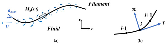
Figure 1.
(a) Schematic diagram of the model problem. (b) Enlarged view of an isolated element corresponding the one represented by a dashed box in (a).
This model is very different from the one we have in the previous works of our group [13,25,26,27], where a single-point actuation is imposed at the leading edge. In the present model, no heaving motion is imposed at the leading edge, while a pitching motion can still be prescribed. Imposing a pitching motion here is solely for the purpose of direction control (in straight-line swimming or steering). This differs significantly from the scenario in [13], where the pitching motion is an indispensable part of the single-point actuation.
2.2. Governing Equations
The fluid flow is assumed to be laminar and is governed by the incompressible Navier–Stokes equations, which can be written in a dimensionless form as
Here all quantities in Equation (1) are scaled by the body length L and characteristic time , where f is the driving frequency of the actuation. is the (dimensionless) velocity of the fluid and p is the (dimensionless) pressure. is the (dimensionless) volume force term, which represents the effect of the propulsor (immersed boundary) on the fluid flow. is the Reynolds number which is defined as , where is the kinematic viscosity coefficient of the fluid.
The motion of the flexible propulsor is governed by the nonlinear structure equations, which can be written in a dimensionless form as
where is the position vector on the flexible body and is the dimensionless Lagrangian forcing term which accounts for the interaction between the propulsor and the fluid. Furthermore, s is the dimensionless Lagrangian coordinate along the arc length. ( and are the coordinates of the leading edge and trailing edge, respectively.) is the unit normal vector on the curved body and is defined as . Here is the unit normal vector which points outwards from the plane, and is the unit tangential vector which points towards the direction of increasing s.
in Equation (2) represents the active bending moment mimicking the actuation of muscle. Here the active bending moment is assumed to take the form of a traveling wave [22,23,24]. The traveling wave is produced as the result of rhythmically passing neural wave of muscle activation from head to tail [21]. The (dimensionless) active moment density , which is the first spatial derivative of , is prescribed as
where A is the dimensionless amplitude of moment density, k is the dimensionless wavenumber. is a weighting function which is defined as . The weighting function is designed such that the values of active moment density are reduced to zero at the two ends. By definition, the dimensionless frequency of wave propagation in Equation (4) equals unity. The active moment can be obtained by
where represents the path from to . The analytical expressions for and are:
It turns out that the values of active moment are also reduced to zero approximately at the two ends.
Aside from the dimensionless wavenumber k, other dimensionless parameters used to describe the system are: the dimensionless amplitude of moment density A, the mass ratio , the dimensionless tension coefficient and the dimensionless bending rigidity . These dimensionless parameters are defined as
where is the characteristic velocity which is defined as . is the linear density of the propulsor and is the density of the fluid. is the dimensional amplitude of moment density. and are the dimensional tension coefficient and bending rigidity, respectively.
The distributions of and along the body can be described by two Gaussian (exponentially decaying) functions as
where the six coefficients are adjusted for obtaining the desirable gait of a carangiform swimming fish [26]. The values of the six coefficients provided in [26], i.e., , are used throughout this work.
3. Numerical Method and Settings
3.1. Numerical Method
We use the direct-forcing immersed boundary method based on discrete stream function formulation to solve the incompressible Navier–Stokes equations (i.e., Equation (1)) [28,29]. The algebraic multigrid method is used to solve the linear systems arising from the discretization. The computer code is parallelized using the message passing interface (MPI) protocol [30]. The inextensible condition (Equation (3)) is satisfied by solving a Poisson-like equation for the dimensionless tension coefficient [11]. The finite difference method is used to discretize the structure equations (including the Poisson-like equation for ) on a staggered grid. For performing fluid-structure interaction (FSI) simulation, we use a loosely coupled scheme [25,26,27]. In this scheme, the fluid equations and structure equations are advanced sequentially by one step in time. The overall accuracies of the temporal and spacial discretizations in the numerical method are first order and second order, respectively.
This in-house FSI code has been thoroughly validated by using a variety of benchmark cases which include the lid-driven cavity flow, the flows over stationary and oscillating cylinders, a sphere, a low-aspect-ratio flat plate and a flapping flag [28,29]. This code has also been used to simulate the self-propelled swimming of a flexible fish-like body [11,25,26,27].
A unit normal vector needs to be defined locally for computing the active force (i.e., the last term of Equation (2)). The three steps involved in computing the local unit normal vector are as follows. First, three consecutive nodes (e.g., , i and ) on the flexible propulsor are used to determine a parabola. Second, the unit tangential vector at node i is determined analytically. Last, the unit normal vector at node i is computed by taking a cross product.
3.2. Numerical Settings
A rectangular computation domain of is used in the simulation (see Figure 2). In solving the fluid equations, the no-slip boundary condition is imposed on the front and back sides of the computational domain, and the free-slip boundary condition is imposed on the top side. The free-slip boundary condition is imposed on the bottom side, in the simulations of the straight-line swimming and the turning maneuver. In the study of the ground effect, the non-slip boundary condition is imposed on the bottom side. For all cases, the no-slip boundary condition is also imposed on the surface of the propulsor by using the direct-forcing immersed boundary method [28]. The initial fluid velocity in the entire domain is set to zero.
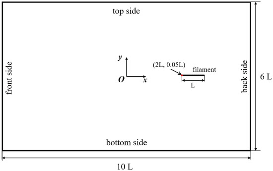
Figure 2.
Computational domain and boundary conditions used in the simulation.
The boundary conditions for the structure equations can be expressed as
where is the deflection angle at the leading edge. is set to zero in the case of straight-line swimming (in an open space or near the ground). is prescribed as a function of time in the case of turning maneuver. In all cases, the trailing edge is treated as a free end. It is worth noting that the leading edge is free of any constraints on its linear displacement. This is very different from the scenario in which a heaving motion is prescribed at the leading edge [13,25,27]. The initial shape of the swimmer is a horizontally oriented straight line, and the initial velocity of the swimmer is set to zero.
A uniform Cartesian mesh with a grid width of is used in the simulation. The total number of cells in the Cartesian mesh is about million. The grid width of the Lagrangian mesh deployed on the propulsor is also . Under such mesh resolution, at least 20 grid points are employed to resolve the shear layers with large velocity gradient (in the zone near the surface of the swimmer and in the narrow gap between the swimmer and the ground). This is sufficient for simulating laminar flows at Reynolds numbers of the order . The time-step used in the simulation is . To ensure that the solutions are independent of the mesh, time-step and domain size, numerical tests are conducted and the results are presented in Appendix A.
4. Results and Discussion
4.1. Controls Parameters and Netrics of Performance
The physical parameters in the simulations are listed in Table 1. The ranges of k and A are determined by trial and error to facilitate efficient locomotion and production of a fish-like swimming gait. The range of Reynolds number is chosen based on the following facts: (a) in this range the flow physics is relatively insensitive to Reynolds number, (b) small Reynolds numbers make the simulation more tractable.

Table 1.
Physical parameters used in the simulations.
Three key dimensionless parameters are used to assess the propulsive performance, i.e., the cruising speed , the fluid power , and the cost of transport per unit mass . The cruising speed is the time-averaged horizontal velocity at the leading edge. The fluid power is the time-averaged power required to produce the oscillation and the forward motion. It can be measured approximately by the time-averaged rate of work done to the fluid. The cost of transport per unit mass is the energy required for a unit mass to travel a unit distance. Mathematically, the definitions of the three parameters can be expressed as
where is the horizontal component of the position vector, T is the dimensionless period (which has the value of unity). These three parameters are evaluated after a periodically steady state is reached.
4.2. Straight-Line Swimming
In this section, we investigate into the steady straight-line swimming in an open space. The parameters used in the simulation are: . The time histories of the horizontal and vertical velocities at the leading edge are shown in Figure 3. It is seen that both velocity components reach a periodic state after a transient phase. The cruising velocity is , while the time-averaged vertical velocity is 0.005, which is very close to zero. This indicates that steady straight-line swimming in the horizontal direction is achieved. The amplitudes of fluctuation in the horizontal and vertical velocity components are approximately and , respectively.
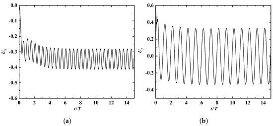
Figure 3.
Time histories of the leading-edgeleading-edge’s horizontal (a) and vertical (b) velocity components in straight-line swimming.
The time histories of the horizontal and vertical fluid forces on the swimmer are shown in Figure 4. Both force components also reach a periodic state after a transient phase. The time-averaged values of the horizontal and vertical components are 0.036 and 0.009, respectively, which are also very close to zero. This further provides a supporting evidence that the state of steady straight-line swimming has been achieved. The slight deviations from zero in the two force components are due to the influence of the active moment and the deflection-angle boundary condition that is imposed at the leading edge.
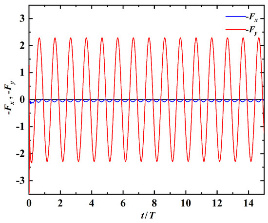
Figure 4.
Time histories of the horizontal and vertical components of fluid force on the propulsor in straight-line swimming.
From Figure 3 and Figure 4, it is seen that the horizontal velocity (or force) component has a frequency which is twice that of the vertical component. This can be explained by the spatio-temporal symmetry (i.e., reflective symmetry after half of the actuation period) which exists in the flow field. Figure 5a,b show the vorticity contours and shapes of the swimmer when the tail reaches its highest and lowest vertical positions, respectively. From these figures, a reverse Karman vortex street with ‘2S’ wake structure is visible. Here the term ‘2S’ refers to the situation in which two vortices of opposite signs are shed per period. This type of wake structure is widely observed in flapping-foil systems, including self-propelled flexible swimmers driven by other types of actuation [13,26].
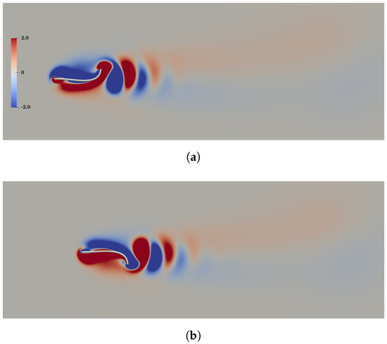
Figure 5.
Vorticity contours and shapes of the swimmer with the trailing edge located at the highest (a) and lowest (b) vertical positions.
The swimming gait during one period of actuation is illustrated in Figure 6. This swimming gait somewhat resembles that of a carangiform swimmer which possesses an inflexible anterior part and a flexible posterior part. In Ref. [26], a similar swimming gait has been produced by using a flexible filament with similar distributions of mass ratio and bending rigidity, but with an imposed leading-edge heaving motion for the actuation. The only difference between them is that the (passive) leading-edge amplitude achieved here is much higher than that of the heaving motion prescribed in [26].
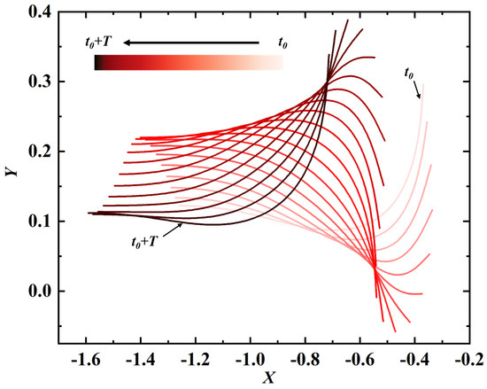
Figure 6.
Shapes of the propulsor at different time instants within one period. The change of color from light to dark in the shapes signifies the increase of time. and T are the initial time instant and the dimensionless period.
Here, the effects of the control parameters on the swimming performance are also explored. First, the effect of wavenumber is investigated by varying k in the range of to , while fixing A and at 200 and 100, respectively. Figure 7 shows the cruising speed and the cost of transport as a function of k. It is seen that both and decrease monotonically with increasing k. The explanation on the inverse proportionality between and k is as follows. The cruising speed is positively correlated with the propagation speed of the traveling wave in the kinematics (swimming gait), at least within certain parameter range [13]. It is reasonable to believe that the wavespeed of the traveling wave in the kinematics is positively correlated with the wavespeed of the active moment. Obviously, this wavespeed is proportional to the wavelength of the active moment imposed, which is inversely proportional to k.
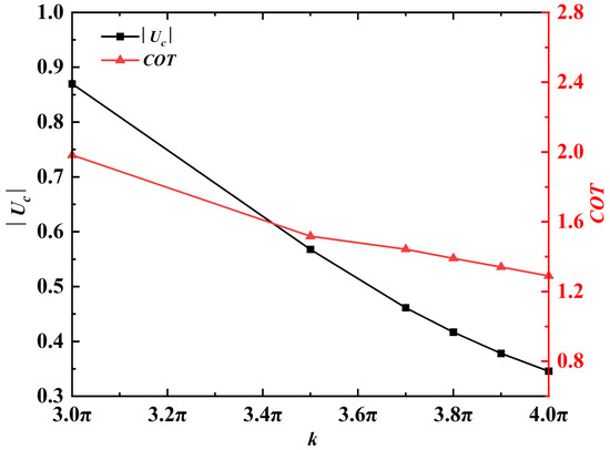
Figure 7.
and as a function of k. The absolute value of is plotted here since the propulsor is swimming in the negative x-direction.
To examine the patterns of motion at different k, amplitude envelopes are created by a superposition of instantaneous body shapes within a period while removing the horizontal displacements, and the results are shown in Figure 8. The ratio of trailing-edge amplitude to leading-edge amplitude is an important parameter for characterising the kinematics. The amplitude ratios at different values of k are listed in Table 2. It is seen that the amplitude ratio is approximately a constant. From Figure 8, it is also observed that the equilibrium vertical position differs with varying k. This is because the time courses of velocity evolution before reaching the ultimate steady state are different.
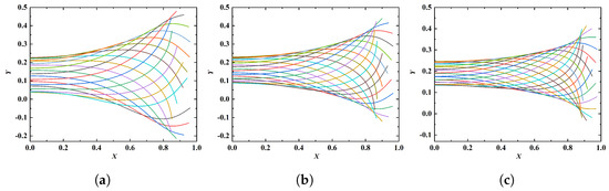
Figure 8.
Amplitude envelopes at different values of k: (a) , (b) , (c) . The fixed parameters are: , .
Table 2.
The amplitude ratios at different wavenumbers.
Next, the influence of A on swimming performance is investigated by varying A in the range of 100–300, while fixing k and at and 100, respectively. Figure 9 shows the variations of and as a function of A. It can be seen that both and increase monotonically with increasing A.
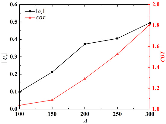
Figure 9.
and as a function of A. The absolute value of is plotted here since the propulsor is swimming in the negative x-direction.
The amplitude envelopes at different A are shown in Figure 10, while the amplitude ratio at different A are listed in Table 3. It is seen that the amplitude ratio is positively correlated with the value of A. The increase of amplitude ratio is the reason why the cruising speed increases with increasing A. It is worth noting that the wave speed is not affected by the variation of A. Similar to Figure 8, it is seen that the equilibrium vertical position differs with varying A. The influence A on the equilibrium vertical position can also be explained by different time courses of velocity evolution at different A.
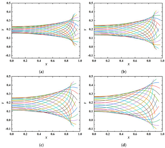
Figure 10.
Amplitude envelopes at different values of A: (a) 150, (b) 200, (c) 250, (d) 300. The fixed parameters are: , .
Table 3.
Amplitude ratios at different values of A.
Finally, to explore the influence of on swimming performance, four Reynolds numbers, namely, 50, 100, 150, 200, are selected. The values of k and A are fixed at and 200, respectively. Figure 11 shows the variations of and as a function of . It is seen that the cruising speed increases while decreases with increasing Reynolds number. The decreased with increasing can be attributed to the reduction of work done to the fluid due to the weakened viscous effect. It is also observed that the variation of Reynolds number has little influence on the kinematics of the swimmers. (The amplitude envelopes are not shown here for brevity.) Similar to the influences of k and A, the equilibrium vertical position is also affected by the variation of . Again, this can be explained by different time courses of velocity evolution at different . The time histories of horizontal velocity at the leading-edge for different values of are shown in Figure 12. It is seen that the larger the value of , the longer the time it takes to reach the steady state.
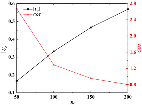
Figure 11.
and as a function of . The absolute value of is plotted since the propulsor is swimming in the negative x-direction.
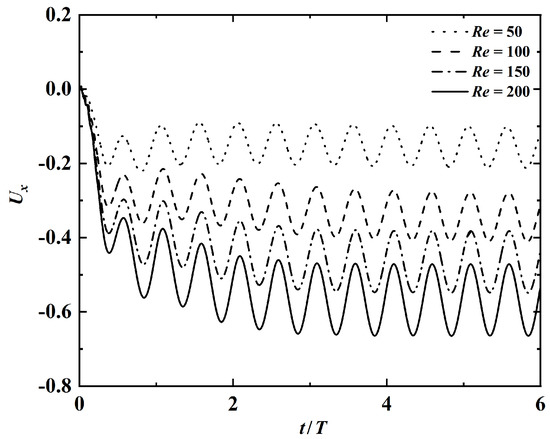
Figure 12.
Time histories of the leading-edge’s horizontal velocity at different values of . The fixed parameters are: , .
4.3. Locomotion near a Solid Wall
In this section, we investigate the ground effect on the swimming performance by considering the case of . The degree of wall proximity is quantified by the distance between the initial y-position of the leading edge and the solid wall underneath. The range of dimensionless wall distance (wall distance scaled by L) considered here is 0.4–3.0. The trailing edge may touch the solid wall if , while the ground effect becomes insignificant if .
Figure 13 shows the time histories of the leading edge’s horizontal velocity at and . It is seen that for the case of , the state of steady swimming is reached approximately after . For the case of , the swimmer keeps accelerating and the state of steady swimming has not been reached even after . The averaged speeds computed using the data in time interval – are and , for and , respectively. Moreover, the computed using the data in time interval – are and , for and , respectively. This indicates that the ground effect enhances both the cruising speed and the energy efficiency.
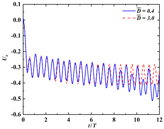
Figure 13.
Time histories of the leading-edge’s horizontal velocity at and .
From the time history of horizontal velocity at the leading edge for , both f and are identified as the dominant frequencies. This is in contrast with the case of , in which only is identified as the dominant frequency. This phenomenon is related to the fact that the ground effect breaks the spatial-temporal symmetry of the flow field. The instantaneous vorticity contours for the case of is shown in Figure 14. It is clearly seen that a reverse Karman vortex street with upward deflection is produced. In the narrow gap between the propulsor and the solid wall, high vorticity concentration is also observed. The vorticity contours shown here share some similarities with those presented in [25], where the ground effect on a self-propelled flexible swimmer driven by a single-point actuation was explored.
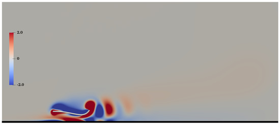
Figure 14.
Vorticity contours for the case of . The black bold horizontal line is the solid wall.
After further investigation, it is found that for the case of , the tail of the swimmer eventually touches the ground after . The time history of the leading-edge’s vertical position is shown in Figure 15. The ‘suction’ induced by the ground effect can be explained by the asymmetry in the active force (i.e., the last term of Equation (2)). The averaged y-component of the active force on the swimmer in time interval is for the case of . This value is much larger than that for the case of (which is ). The asymmetry in active force is caused by the (slightly) asymmetric shapes (swimming gaits) (see Figure 16). In this figure, the black and red solid lines denote the shapes of the propulsor at and , respectively. The black dashed line denotes the mirror image of the shape at . The cyan lines denote the shapes of the propulsor at eight uniformly-spaced instants in time interval [, ]. It is worth noting that the time-averaged y-components of the fluid force are almost identical (and close to zero), with either strong or insignificant ground effect.
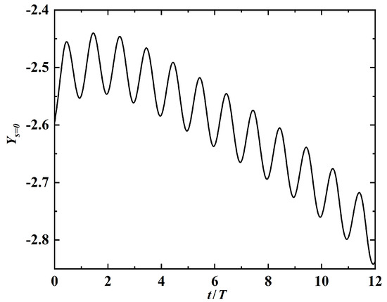
Figure 15.
Time history of the leading-edge’s y-displacement at .
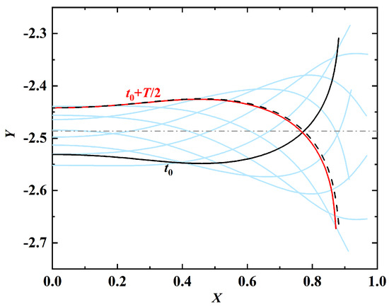
Figure 16.
Asymmetry in the shapes (swimming gaits) of the propulsor induced by the strong ground effect at .
In order to avoid collision during swimming in close proximity to the wall and eventually reach a periodically steady state, the kinematics of the swimmer needs to be fine-tuned [31] to counteract the asymmetry aforementioned. This can be achieved through a slight modification to the form of the imposed active moment, in combination with a control law for the deflection angle at the leading edge.
4.4. Turning Maneuver
In this section, we design a strategy for the swimmer to perform a turning maneuver by treating the leading edge as a ‘rudder’. To this end, the leading-edge deflection angle is assumed to obey the following evolution law:
where is the deflection angle after turning, is a parameter which controls the elapsed time to complete the turn, is a parameter which controls the start time of the turning maneuvering. Equation (11) can facilitate a smooth transition of the deflection angle between zero and in a given time interval. The time variation of with is shown in Figure 17. To ensure a sufficient temporal resolution in simulating the turning maneuver, the time-step should be much smaller than the characteristic time of the transition process. This is satisfied since the characteristic time of transition is of the order of 1, while the time-step used in the simulation is .
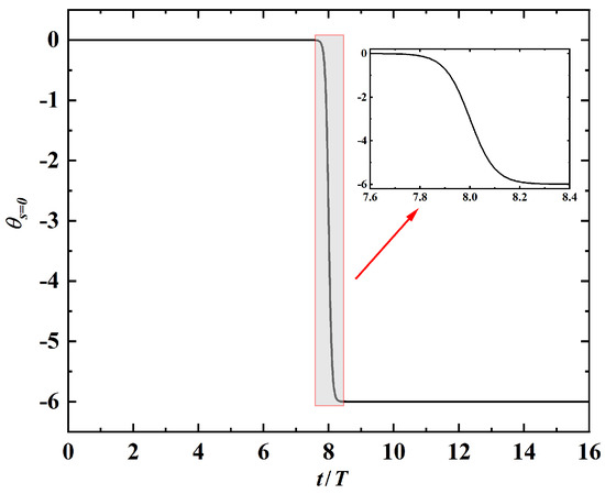
Figure 17.
Variation of leading-edge deflection angle as a function of time in the turning maneuver. A enlarged view of the part of the curve in time interval is shown in the inset.
The parameters used in performing the simulation of turning maneuver with are: . Figure 18 shows the time history of the leading-edge’s vertical velocity. In the first seven periods, the time-averaged vertical velocity is approximately zero. This is indicative of steady straight-line swimming in the horizontal direction. From the seventh period to the ninth period, the propulsor starts to make a right turn and the time-averaged vertical velocity gradually increases from zero to . After the ninth period, steady straight-line swimming in a obliquely upward direction is achieved and the turning maneuver is completed. The instantaneous vorticity contours at , and as shown in the Figure 19. From this figure, it is clearly seen that the horizontally oriented vortex street is gradually transited into a downward deflected one after the turning maneuver.
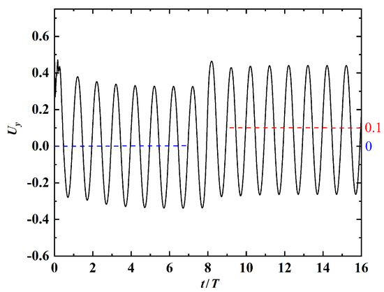
Figure 18.
Time history of the leading-edge’s vertical velocity. The blue and red dashed lines denote the time-averaged velocities before and after the turning maneuver.
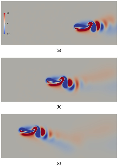
Figure 19.
Vorticity contours at (a), (b) and (c) in the turning maneuver with .
The turning maneuvers with different values of , namely, are also simulated. The actual and period-averaged trajectories of the leading edge at different values of are shown in Figure 20. Here the magnitude of turning is quantified by the turning angle (), which is defined as the angle between the swimming directions before and after the turning maneuver. Figure 21 shows the relation between and . It is seen that the two angles are (almost) linearly proportional to one another in the parameter range of this study.
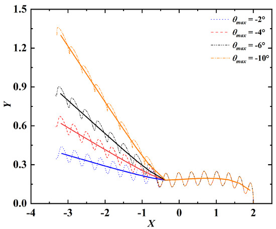
Figure 20.
Trajectories of the leading edge for turning maneuvers with different values of . The dashed lines represent the actual trajectories. The solid lines represent the trajectories after periodic averaging.
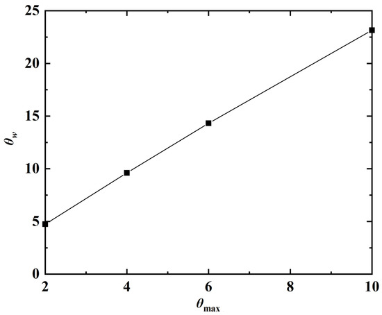
Figure 21.
Relation between and . The black solid line in the line of best fit.
5. Conclusions
In this paper, we present a computational framework for assessing the swimming performance of a flexible propulsor driving by a distributed active moment. The immersed boundary method is employed to conducted the fluid-structure interaction simulation. To mimic the muscle actuation, the active moment imposed on the body of the propulsor takes the form of a traveling wave. Three types of swimming, namely, straight-line swimming in a open space, near-wall swimming and turning maneuver, are explored.
In the straight-line swimming, the ranges of wavenumber and amplitude of the moment density are – and 100–300, respectively. The Reynolds numbers based on the actuation frequency and body length are in the range of 50–200. It is found that the cruising speed and cost of transport are inversely proportional to the wavenumber and proportional to the amplitude of moment density. The cruising speed is proportional to the Reynolds number, while the cost of transport is inversely proportional to the Reynolds number.
In the near-wall swimming, the dimensionless wall distances considered are in the range of –. It is found that in the case with strong ground effect (), the cruising speed is enhanced while the cost of transport is reduced simultaneously. It is also found that for the case of , the tail of the propulsor eventually collides with the ground after 13 actuation periods. In order to avoid collision when swimming in close proximity to the wall, the propulsor’s kinematics needs to be fine-tuned.
A simple evolution law for the leading-edge deflection angle is designed to achieve the turning maneuvers. The deflection angle is allowed to change steeply by an amount in the range of to in approximately one actuation period. As a result, the turning maneuvers with turning angles ranging from to are completed in approximately two actuation periods.
In our future work, control strategies will be designed for the swimmer to perform more complex tasks, such as position keeping in vortical flows, steady near-wall swimming free of collision, point-to-point navigation and obstacle avoidance maneuvering. The most promising solution to the challenging problems aforementioned is the artificial intelligence (AI) control based on deep reinforcement learning (DRL).
Author Contributions
Conceptualization, X.Z. and C.H.; methodology, C.H. and X.Z.; software, C.H.; validation, C.H. and Z.Z.; formal analysis, C.H., Z.Z. and X.Z.; investigation, C.H.; resources, X.Z.; data curation, C.H. and X.Z.; writing—original draft preparation, C.H. and X.Z.; writing—review and editing, X.Z., C.H., Z.Z.; visualization, C.H.; supervision, X.Z.; project administration, X.Z.; funding acquisition, X.Z. All authors have read and agreed to the published version of the manuscript.
Funding
This research was funded by the National Natural Science Foundation of China under grant numbers 11372331, 11772338, and 12172361 and by the Chinese Academy Sciences under the grant numbers XDB22040104 and XDA22040203.
Institutional Review Board Statement
Not applicable.
Informed Consent Statement
Not applicable.
Data Availability Statement
Not applicable.
Conflicts of Interest
The authors declare no conflict of interest.
Appendix A. Mesh, Time-Step and Domain Independence Tests
To test the mesh independence of the solutions, three uniform meshes of different resolutions are generated. The detailed information of the meshes used in the test are summarized in Table A1. The straight-line swimming with is simulated by using the three meshes. The time histories of the leading-edge’s horizontal velocity and the horizontal fluid force on the propulsor obtained using the three meshes are shown in Figure A1. The convergence behavior is clearly seen from the solutions obtained using the medium and fine meshes.
Similarly, to test the time-step independence of the solutions, simulation is also performed on the medium mesh with a grid width of , by using time-steps of three different sizes (i.e., ). The time histories of the leading-edge’s horizontal velocity and the horizontal fluid force on the propulsor obtained with the three time-step sizes are shown in Figure A2. It is clearly seen that the three solutions are almost indistinguishable.
Finally, a domain independence test is conducted on the same case. We generate three computational domains with different size. The medium mesh and the medium time-step size are used in the simulation. It turns out that the results obtained with the three domains are almost indistinguishable (see Figure A3).
To summarize, the solutions that are independent of mesh, time-step and domain size can be achieved with the spatial resolution of , temporal resolution of and domain size of .
Table A1.
Information of the meshes used in the mesh independence test.
Table A1.
Information of the meshes used in the mesh independence test.
| Mesh 1 | Points per Chord Length | Total Grid Points (Million) |
|---|---|---|
| C | 101 | 0.6 |
| M | 201 | 2.4 |
| F | 301 | 5.4 |
1 C: coarse mesh; M: medium mesh; F: fine mesh.

Figure A1.
Time histories of (a) the leading-edge’s horizontal velocity and (b) horizontal fluid force, obtained by using three different meshes.
Figure A1.
Time histories of (a) the leading-edge’s horizontal velocity and (b) horizontal fluid force, obtained by using three different meshes.


Figure A2.
Time histories of (a) the leading-edge’s horizontal velocity and (b) the horizontal fluid force, obtained by using three different time−step sizes.
Figure A2.
Time histories of (a) the leading-edge’s horizontal velocity and (b) the horizontal fluid force, obtained by using three different time−step sizes.


Figure A3.
Time histories of (a) the leading-edge’s horizontal velocity and (b) the horizontal fluid force, obtained by using three computational domains with different size.
Figure A3.
Time histories of (a) the leading-edge’s horizontal velocity and (b) the horizontal fluid force, obtained by using three computational domains with different size.

References
- Wu, X.; Zhang, X.; Tian, X.; Li, X.; Lu, W. A review on fluid dynamics of flapping foils. Ocean. Eng. 2020, 195, 106712. [Google Scholar] [CrossRef]
- Lauder, G.V.; Anderson, E.J.; Tangorra, J.; Madden, P.G. Fish biorobotics: Kinematics and hydrodynamics of self-propulsion. J. Exp. Biol. 2007, 210, 2767–2780. [Google Scholar] [CrossRef] [PubMed]
- Wang, S.Z.; He, G.W.; Zhang, X. Self-propulsion of flapping bodies in viscous fluids: Recent advances and perspectives. Acta Mech. Sin. 2016, 32, 980–990. [Google Scholar] [CrossRef]
- Lin, X.J.; Wu, J.; Zhang, T.W. Self-directed propulsion of an unconstrained flapping swimmer at low Reynolds number: Hydrodynamic behaviour and scaling laws. J. Fluid Mech. 2020, 907, R3. [Google Scholar] [CrossRef]
- Lucas, K.N.; Johnson, N.; Beaulieu, W.T.; Cathcart, E.; Tirrell, G.; Colin, S.P.; Gemmell, B.J.; Dabiri, J.O.; Costello, J.H. Bending rules for animal propulsion. Nat. Commun. 2014, 5, 3293. [Google Scholar] [CrossRef]
- Erturk, A.; Delporte, G. Underwater thrust and power generation using flexible piezoelectric composites: An experimental investigation toward self-powered swimmer-sensor platforms. Smart Mater. Struct. 2011, 20, 125013. [Google Scholar] [CrossRef]
- Gao, B.F.; Guo, S.X. Dynamic mechanics and electric field analysis of an ICPF actuated fish-like underwater microrobot. In Proceedings of the 2011 IEEE International Conference on Automation and Logistics (ICAL), Chongqing, China, 15–16 August 2011; pp. 330–335. [Google Scholar]
- Wang, C.; Tang, H.; Zhang, X. Fluid-structure interaction of bio-inspired flexible slender structures: A review of selected topics. Bioinspiration Biomim. 2022, 17, 041002. [Google Scholar] [CrossRef]
- Kern, S.; Koumoutsakos, P. Simulations of optimized anguilliform swimming. J. Exp. Biol. 2006, 209, 4841–4857. [Google Scholar] [CrossRef]
- Hua, R.N.; Zhu, L.D.; Lu, X.Y. Locomotion of a flapping flexible plate. Phys. Fluids 2013, 25, 121901. [Google Scholar] [CrossRef]
- Zhu, X.J.; He, G.W.; Zhang, X. Numerical study on hydrodynamic effect of flexibility in a self-propelled plunging foil. Comput. Fluids 2014, 97, 1–20. [Google Scholar] [CrossRef]
- Kim, B.; Park, S.G.; Huang, W.; Sung, H.J. Self-propelled heaving and pitching flexible fin in a quiescent flow. Int. J. Heat Fluid Flow 2016, 62, 273–281. [Google Scholar] [CrossRef]
- Li, B.L.; Wang, Y.W.; Yin, B.; Zhang, X.; Zhang, X. Self-propelled swimming of a flexible filament driven by coupled plunging and pitching motions. J. Hydrodyn. 2021, 33, 157–169. [Google Scholar] [CrossRef]
- Wu, W. Study on the propulsion of the rigid-flexible composite plate driven on two points. Fluid Dyn. Res. 2022, 54, 035501. [Google Scholar] [CrossRef]
- Luo, Y.; Wright, M.; Xiao, Q.; Yue, H.; Pan, G. Fluid-structure interaction analysis on motion control of a self-propelled flexible plate near a rigid body utilizing PD control. Bioinspiration Biomim. 2021, 16, 066002. [Google Scholar] [CrossRef] [PubMed]
- Kim, B.; Park, S.G.; Huang, W.; Sung, H.J. An autonomous flexible propulsor in a quiescent flow. Int. J. Heat Fluid Flow 2017, 68, 151–157. [Google Scholar] [CrossRef]
- Lin, Z.; Hess, A.; Yu, Z.; Cai, S.; Gao, T. A fluid-structure interaction study of soft robotic swimmer using a fictitious domain/active-strain method. J. Comput. Phys. 2019, 376, 1138–1155. [Google Scholar] [CrossRef]
- Hess, A.; Tan, X.; Gao, T. CFD-based multi-objective controller optimization for soft robotic fish with muscle-like actuation. Bioinspiration Biomim. 2020, 15, 035004. [Google Scholar] [CrossRef]
- Curatolo, M.; Teresi, L. Modeling and simulation of fish swimming with active muscles. J. Theor. Biol. 2016, 409, 18–26. [Google Scholar] [CrossRef]
- Hoover, A.P.; J. Daniels, J.; Nawroth, J.C.; Katija, K. A computational model for tail undulation and fluid transport in the giant larvacean. Fluids 2021, 6, 88. [Google Scholar] [CrossRef]
- Cheng, J.Y.; Pedley, T.J.; Altringham, J.D. A continuous dynamic beam model for swimming fish. Philos. Trans. R. Soc. London. Ser. Biol. Sci. 1998, 353, 981–997. [Google Scholar] [CrossRef]
- Zhang, W.; Yu, Y.L.; Tong, B.G. Fish swimming: Patterns in the mechanical energy generation, transmission and dissipation from muscle activation to body movement. AIP Conf. Proc. 2011, 1376, 476–479. [Google Scholar]
- Gazzola, M.; Argentina, M.; Mahadevan, L. Gait and speed selection in slender inertial swimmers. Proc. Natl. Acad. Sci. USA 2015, 112, 3874–3879. [Google Scholar] [CrossRef] [PubMed]
- Gross, D.; Roux, Y.; Argentina, M. Curvature-based, time delayed feedback as a means for self-propelled swimming. J. Fluids Struct. 2019, 86, 124–134. [Google Scholar] [CrossRef]
- Dai, L.; He, G.; Zhang, X. Self-propelled swimming of a flexible plunging foil near a solid wall. Bioinspiration Biomim. 2016, 11, 046005. [Google Scholar] [CrossRef]
- Dai, L.; He, G.; Zhang, X.; Zhang, X. Stable formations of self-propelled fish-like swimmers induced by hydrodynamic interactions. J. R. Soc. Interface 2018, 15, 20180490. [Google Scholar] [CrossRef]
- Dai, L.; He, G.; Zhang, X.; Zhang, X. Intermittent locomotion of a fish-like swimmer driven by passive elastic mechanism. Bioinspiration Biomim. 2018, 13, 056011. [Google Scholar] [CrossRef]
- Wang, S.; Zhang, X. An immersed boundary method based on discrete stream function formulation for two-and three-dimensional incompressible flows. J. Comput. Phys. 2011, 230, 3479–3499. [Google Scholar] [CrossRef]
- Zhu, X.; He, G.; Zhang, X. An improved direct-forcing immersed boundary method for fluid-structure interaction simulations. J. Fluids Eng. 2014, 136, 040903. [Google Scholar] [CrossRef]
- Wang, S.; He, G.; Zhang, X. Parallel computing strategy for a flow solver based on immersed boundary method and discrete stream-function formulation. Comput. Fluids 2013, 88, 210–224. [Google Scholar] [CrossRef]
- Liu, L.; Zhong, Q.; Han, T.; Moored, K.W.; Quinn, D.B. Fine-tuning near-boundary swimming equilibria using asymmetric kinematics. Bioinspiration Biomim. 2022, 18, 016011. [Google Scholar] [CrossRef]


Disclaimer/Publisher’s Note: The statements, opinions and data contained in all publications are solely those of the individual author(s) and contributor(s) and not of MDPI and/or the editor(s). MDPI and/or the editor(s) disclaim responsibility for any injury to people or property resulting from any ideas, methods, instructions or products referred to in the content. |
© 2023 by the authors. Licensee MDPI, Basel, Switzerland. This article is an open access article distributed under the terms and conditions of the Creative Commons Attribution (CC BY) license (https://creativecommons.org/licenses/by/4.0/).