Evaluation of SPH and FVM Models of Kinematically Prescribed Peristalsis-like Flow in a Tube

Abstract

Peristaltic flow is important in many biological processes, including digestion, and forms an important component of any in silico model of the stomach. There is a clear need to verify the simulations of such flows. An analytical solution was identified that can be used for model verification, which gives an equation for the net volumetric flow over a cycle for an applied sinusoidal wall motion. Both a smooth particle hydrodynamics (SPH) code (from the CSIRO), which is being used to develop a stomach model that includes wall motion, buoyancy, acid secretion and food breakdown, and the Ansys Fluent Finite Volume Method (FVM) solver, that is widely used in industry for complex engineering flows, are used in this exercise. Both give excellent agreement with the analytic solution for the net flow over a cycle for a range of occlusion ratios of 0.1–0.6. Very similar velocity fields are obtained with the two methods. The impact of parameters affecting solution stability and accuracy are described and investigated. Having validated the moving wall capability of the SPH model it can be used with confidence in stomach simulations that include wall motion.

1. Introduction

Peristaltic flow arises when a series of contraction and expansion movements propagate along elastic tube-shaped structures. The fluid and/or solid content inside moves along with the wave as it propagates. In physiology, peristaltic waves are generated by the longitudinal and circular muscular fibers along the wall [1]. This motion is essential in the digestive system for its role in transporting and mixing food/nutrients in the gastrointestinal tract (GIT) [2,3,4,5,6]. The peristaltic motor patterns in the human gut are very complex and governed by multiple mechanisms and factors, including muscle activity, the thickness of the muscularis, and muscle tissue characteristics (elasticity, contractility, extensibility) [7,8,9,10].

In vivo studies provide the most relevant insights into the digestion process due to the complexity and inter-person variabilities of the digestion system. Researchers usually use animal models to study digestion because human subjects are not easy to recruit, experiments are hard to perform and to get measurements from, and complex ethical approval is required [11]. Even though animal models are often used as an alternative to humans [12,13,14,15], they do not necessarily accurately reflect the human situation and still require strict ethics approval and specific technical skills. Therefore, in vitro models (e.g., test tube-based or similar) are designed to replicate the digestion process. These experimental studies are constructed with an aim to replicate the fluid flow conditions, shear stresses and complex chemistry in the GIT. Detailed reviews of in vitro digestion models are provided by Li et al. [16], Zhong and Langrish [17], Bornhorst and Singh [11], Dupont et al. [18] and Hur et al. [19]. In vitro models allow control of many factors that cannot be controlled in the in vivo system [11], which affords a better systematic understanding of individual factors.

However, these experimental systems can be hard to design to replicate local flow and concentration fields that occur in the body and can be very hard to customize to represent in vivo scenarios. With the massive improvements in numerical methods and computing power over the last few decades, in silico methods have the huge advantage that local data can be obtained for all variables, such as velocity, pressure, and species concentration [3,4,6,20,21,22,23]. Therefore, if a suitably accurate computational model of an in vivo system can be constructed, the in silico results can provide insights into the in vivo system behavior. Although the primary aim is to understand in vivo behavior, in silico models can guide in vitro experimental design after being validated by data from the in vitro model. This synergistic approach is important in model developments that utilize in silico models that benefit from the verification work performed here. Ultimately, the in silico and in vitro work will lead to in silico models that can simulate the full digestion process happening in the human stomach.

In the past two decades, many numerical models of this process based on Computational Fluid Dynamics (CFD) methods have been developed. Models have been built for different parts of the GI tract, including the esophagus [24], stomach [4,25,26] and intestine [3,20,21,22,23,27,28]. These models provide valuable insights into the flow pattern of the digestion content, which is not easily quantified in both in vivo and in vitro studies. In the early developed models, single-phase fluid was simulated with various densities and viscosities. Recently, multiphase flow simulations (including with free surfaces and particles) have been implemented and improved by Sinnott et al. [3] and Harrison et al. [4]. Some models also include gastric secretion [6] and electrophysiology [27]. The developed models have demonstrated their capability and high potential in simulating this complex system but, to date, lack systematic validation for replicating physical outcomes. It is therefore important to verify and validate the components of established models to demonstrate their accuracy and stability.

An analytical solution [29], described later, can be used to calculate the detailed peristaltic-induced fluid motion for an idealized tube geometry. However, numerical analysis is needed to understand complicated systems, such as the intestine and the stomach, which involve the combination of fluid flow, free surfaces, complex boundary conditions, and solids content. The capability of SPH in simulating the digestion model has been demonstrated in the intestine models developed using the CSIRO SPH code [3,20,21,22,23,28] and the stomach model developed by Harrison et al. [4]. Peristaltic flow is a fundamental component of all these models, and it is therefore useful to validate computational models for this process and then to perform additional validation as more physics is added, knowing that the underlying moving wall flow model is well validated.

The main aim of this paper is to validate the accuracy of the smooth particle hydrodynamics (SPH) method when applied to the peristaltic motion of a single-phase Newtonian fluid. Once the model is validated for this simple system, it will provide a high level of confidence for other applications, where peristalsis is involved in more complicated systems. The Finite Volume method (FVM) is also employed in the study and acts as a comparison approach. Compared with the novel mesh-free SPH method, FVM is a traditional mesh-based method that has been well-established for decades [30]. By comparing the performance of both numerical methods, their accuracy and efficiency can be explored.

2. Analytical Solution

Several studies have investigated flow in a tube during simplified peristalsis driven by a moving wall [1,29,31,32]. Under constrained flow conditions the flow field and pressure distribution can be calculated from the amplitudes of the wall deformations only. In this study, the analytical solution of Shapiro et al. [29] is used to validate the numerical models of peristalsis. A continuous sinusoidal wave train moving in one direction along the tube axis with a constant speed is used to determine the instantaneous shape of a moving boundary wall on a tube of uniform initial diameter. The applied motion generates a volumetric flow which can be compared with analytic results. An illustration of the fluid-filled tube, which has a deforming wall that is one wavelength long, is shown in Figure 1.

In the simulations, the wavelength $\lambda$ of the imposed wave is specified, which is related to the wavenumber by:

$$k=\frac{a }{\lambda }$$

(1)

where $a$ is the radius of the tube. Using these definitions, a Reynolds number can be formed as

$$Re=\frac{\rho ac}{\mu }\times \frac{a}{\lambda }$$

(2)

where $c$ is the speed of the imposed wave, $\mu$ is the dynamic viscosity and $\rho$ is the fluid density.

The analytical model assumes a continuous train of waves and inertia-free fluid flow, which requires two criteria to be met. Firstly, the wavenumber ($k$), which is the ratio of the radius to the wavelength, should be close to zero, as it is assumed to be zero in the analytical solution. Under this condition, the transverse velocities and pressure gradients are negligible compared with their longitudinal counterparts. Secondly, the Reynolds number ($Re$), which gives the ratio of inertial to viscous forces must be close to zero, as it is again assumed to be zero in the analytical solution.

From Fung and Yih [1], the equation for the imposed peristaltic waves is:

$$b\left(x,t\right)=a\varphi \sin 2\pi \left(\frac{x-ct}{\lambda }\right)$$

(3)

where $b\left(x,t\right)$ denotes the wall deformation in the radial direction, $x$ is the longitudinal location, $t$ is time and $\varphi =b/a$ is the amplitude ratio, which is set to a range of 0.1 to 0.6, corresponding to occlusions of 10% to 60%, deemed to be sufficient given the purpose of this study.

The effect of changing the amplitude ratio, $\varphi$, on the fluid flow is investigated. In the analytical solution, the fluid is assumed to be incompressible. The fluid flows through the tube with constant static pressure at the tube boundaries. The dimensionless time-average volumetric flow rate ($\dot{V}$) is a good measure of the flow behaviour and is dependent on the amplitude ratio ($\varphi$) [29]:

$$\dot{V}=\frac{\varphi \left(4+\varphi \right)}{2+3{\varphi }^2}$$

(4)

3. Setup of the Numerical Model

3.1. Physiological Parameters

The physiological data for the human ureter [1] are used in the peristalsis model developed in this work. As shown in

Table 1. Parameters used in the numerical models.

Geometrical Dimensions
Radius	a	0.001 m
Length	L	0.05 m
Peristaltic Waves Characteristics
Wave speed	c	0.03 m/s
Wavelength	λ	0.05 m
Amplitude ratio	ϕ	0.1–0.6
Fluid Properties
Dynamic viscosity	μ	0.01 Pa·s
Density	$\rho$	1000 kg/m3
Conditions
The ratio of tube radius to wavelength	k	0.02 (close to 0)
Reynolds number	Re	0.06 (close to 0)

, the input parameters include the tube dimensions, the characteristics of the imposed motion and the properties of the fluid inside the tube. Both the wavenumber and Reynolds number are close to zero as required.

The nodes on the boundary are displaced radially according to the profile given by Equation (3) in both the SPH and FVM simulations. The wall location used in the simulation, $H\left(x,t\right),$ is determined from the imposed wave motion given by $b\left(x,t\right)$ (Equation (3)) with the inclusion of a ramp to start the simulation gradually to prevent mesh distortion:

$$H\left(x,t\right)=a\left(1+\min \left(\frac{t}{t_i}, 1\right)\times \varphi \sin 2\pi \left(\frac{x-ct}{\lambda }\right)\right)$$

(5)

where $t_i$ is the ramp time, set to $\lambda /c$. Results before time $t_i$ are not included when calculating the averaged flow rate.

The following equations are applied to convert the equations into Cartesian coordinates.

$$\theta ={\tan }^{-1}\left(\frac{z}{y}\right)$$

(6)

$$y=H\left(x,t\right)\cos \left(\theta \right)$$

(7)

$$z=H\left(x,t\right)\sin \left(\theta \right)$$

(8)

where $y$ and $z$ are the transformed coordinates in a Cartesian coordinate system.

The problem described above is next set up and solved using both SPH and FVM so that the results can be compared for the same geometry, boundary conditions and fluid properties.

3.2. SPH Model

In the SPH approach, the Navier–Stokes equations are used to solve fluid dynamics problems, with particles representing discrete “lumps” of fluid, that are tracked in a Lagrangian framework. The formulation of the model results in a set of ordinary differential equations describing the motion of fluid particles [33]. More details of the method can be found in Monaghan [34,35] and Cleary et al. [20,33]. The CSIRO SPH code [36] is used in this study.

To obtain values of quantities such as density and velocity at a given point, data must be obtained from the surrounding region. The interpolated value of a function $A$ at a point $\mathit{r}$, is the sum over all particles within a radius of distance related to $h$ from point $\mathit{r}$ [34]:

$$A\left(\mathit{r}\right)={\displaystyle \sum }_b{m}_b\frac{A_b}{{\rho }_b}W\left(\mathit{r}-{\mathit{r}}_b,h\right)$$

(9)

where $A_b$ is the value of $A$ at ${\mathit{r}}_b$, $m_b$ is the mass of fluid particle $b$, and $W$ is an interpolation kernel function with a smoothing length of $h$ evaluated at a distance $\left|\mathit{r}-{\mathit{r}}_b\right|$ from the position of interest. In this work, $h$ is set to be 1.2 times the initial particle separation distance, $\mathsf{\Delta }x$. The concept of a smoothing kernel is shown in Figure 2 below.

The kernel is essential to the entire method as it is used for the calculation of both spatially interpolated values and gradients. The effect of three different kernels is examined in this work for the same smoothing length. The dimensionless distance used in the kernel is defined as

$$\mathsf{\Delta }=\frac{{\mathit{r}}_{ab}}{h}$$

(10)

where ${\mathit{r}}_{ab}$ is the distance between particles $b$ and $a$.

The quartic spline kernel [37] is used for the base case in this study

$$W\left({\mathit{r}}_{ab},h\right)=\frac{1}{20\pi h^3}\left\{\begin{array}{c}{\left(2.5-\mathsf{\Delta }\right)}^4-5{\left(1.5-\mathsf{\Delta }\right)}^4+10{\left(0.5-\mathsf{\Delta }\right)}^4, \mathsf{\Delta }\le 0.5\\ {\left(2.5-\mathsf{\Delta }\right)}^4-5{\left(1.5-\mathsf{\Delta }\right)}^4, 0.5\le \mathsf{\Delta }\le 1.5\\ {\left(2.5-\mathsf{\Delta }\right)}^4, 1.5\le \mathsf{\Delta }\le 2.5\\ 0, \mathsf{\Delta }\ge 2.5\end{array}\right.$$

(11)

The fifth-order Wendland kernel [37,38] is also studied:

$$W\left({\mathit{r}}_{ab},h\right)=\frac{7}{85.336\pi h^3}\left\{\begin{array}{c}{\left(2-\mathsf{\Delta }\right)}^4\left(1+2\mathsf{\Delta }\right), 0\le \mathsf{\Delta }\le 2\\ 0, \mathsf{\Delta }\ge 2\end{array}\right.$$

(12)

as well as the cubic spline kernel [35,39]:

$$W\left({\mathit{r}}_{ab},h\right)=\frac{1}{\pi h^3}\left\{\begin{array}{c}1-\frac{3}{2}{\left(\mathsf{\Delta }\right)}^2+\frac{3}{4}{\left(\mathsf{\Delta }\right)}^3, \mathsf{\Delta }\le 1\\ \frac{1}{4}{\left(2-\mathsf{\Delta }\right)}^3, 1\le \mathsf{\Delta }\le 2\\ 0, \mathsf{\Delta }\ge 2\end{array}\right.$$

(13)

A comparison of the kernel shapes is shown in Figure 3. To display them the dimensionless kernel $W\left({\mathit{r}}_{ab},h\right)h^3$ was plotted as a function of the normalized distance.

From Figure 3 several important observations can be made:

(1)

The value of any variable at a given point depends on all particle values inside a sphere of radius $nh$ centred on that point. In SPH this is usually referred to as a kernel having compact support with radius $nh$. For the cubic and Wendland kernels $n=2,$ and for the quartic kernel $n=2.5$. Therefore, for any given particle configuration the quartic kernel involves summation of more particles over a greater spatial extent than the other two.

(2)

The kernels give different relative weighting to particles closer to the point of interest. This impacts not only the value but also the gradients of variables.

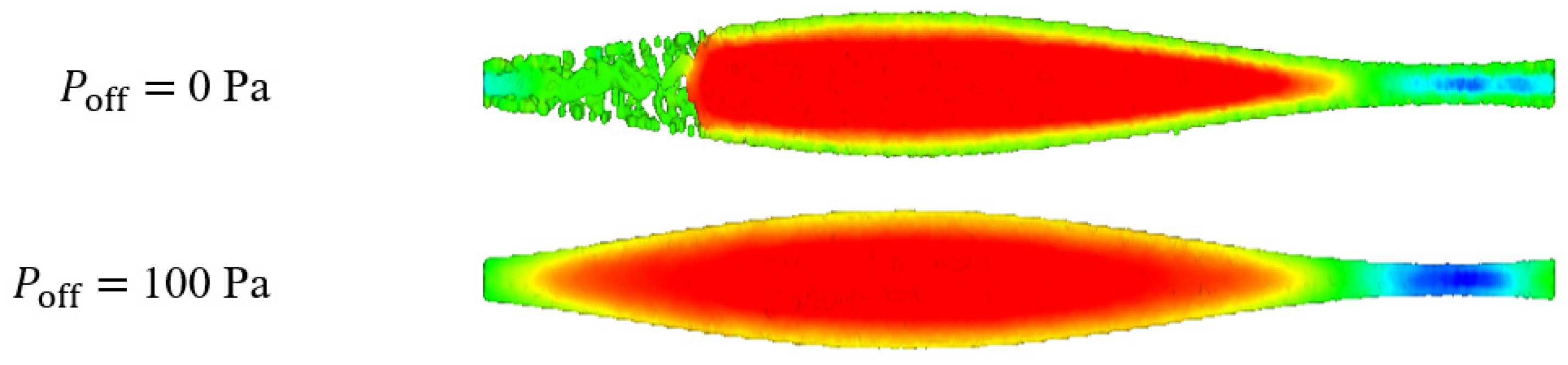
The gradient of the function $A$ is obtained by differentiating Equation (9):

$$\nabla A\left(\mathit{r}\right)={\displaystyle \sum }_b{m}_b\frac{A_b}{{\rho }_b}\nabla W\left(\mathit{r}-{\mathit{r}}_b,h\right)$$

(14)

The conservation equation for mass can then be formulated as [34,40]:

$$\frac{d{\rho }_a}{dt}={\displaystyle \sum }_b{m}_b{\mathit{v}}_{ab}·{\nabla }_a{W}_{ab}$$

(15)

where ${\rho }_a$ is the density of fluid particle $a$, $t$ is time, ${\mathit{v}}_{ab}={\mathit{v}}_a-{\mathit{v}}_b$, is the relative velocity between particles $a$ and $b$.

The fluid pressure can then be calculated based on the particle density. Although the analytic solution is derived for an incompressible fluid, a weakly compressible approach is adopted here and is configured to have low compressibility. This approach is applied by introducing an equation of state of the form:

$$P=P_0\left[{\left(\frac{\rho }{{\rho }_0}\right)}^{\Upsilon }-1\right]+P_{\mathrm{off}}$$

(16)

where $P$ is the fluid pressure; $P_0$ is the pressure scale factor; $\rho$ is the particle density; ${\rho }_0$ is the reference density, set to 1000 kg/m³ for water in this work; $P_{\mathrm{off}}$ is a background pressure that is added to avoid negative pressure values.

Weakly compressible SPH is designed for free surface flow prediction [34] with an essential component being the ability of diverging fluid (which has a negative pressure when calculated by Equation (16) when $P_{\mathrm{off}}=0$) to create new free surface. In a fully enclosed expanding flow this will allow unphysical internal void formation. However, the analytical model assumes that the tube content is a single-phase fluid without internal free surfaces. The equation of state therefore needs to be adapted to ensure that $P>0$ throughout the tube and for the entirety of the simulation. This is achieved by including a pressure offset, $P_{\mathrm{off}},$ which is sufficiently large to guarantee that the pressure remains positive. Since the fluid dynamical force only depends on the pressure gradient, the addition of such a constant has no other effect aside from ensuring the positivity of the pressure.

The effect of this offset pressure in the current work is very important, as shown in Figure 4. Without the offset pressure voids are created, which are not present in the single-phase flow being modelled here. A background pressure of 100 Pa is found to be sufficient to ensure $P>0$ and therefore inhibit this internal free surface generation and is used for all cases.

The pressure scale factor $P_0$ in Equation (16) is given by

$$\frac{\gamma P_0}{{\rho }_0}={c_s}^2={(10V)}^2$$

(17)

where $\gamma$ is 7, which is a material constant defined for water [41]; $c_s$ is the local speed of sound, which needs to be large enough to make sure the density variations are small and the fluid is close to incompressible, but it also needs to be low enough to avoid the need for unnecessarily small timesteps [41] (see later); $c_s$ needs to be at least 10 times larger than the characteristic fluid velocity in the flow field ($V$), which corresponds to a Mach number of 0.1 or smaller and gives a density variation of less than 1% [34].

The conservation equation for momentum becomes:

$$\frac{d{\mathit{v}}_a}{dt}=-{\displaystyle \sum }_b{m}_b\left[\left(\frac{P_b}{{\rho }_b^2}+\frac{P_a}{{\rho }_a^2}\right)-\frac{\xi }{{\rho }_a{\rho }_b}\frac{4{\mu }_a{\mu }_b}{\left({\mu }_a+{\mu }_b\right)}\frac{{\mathit{v}}_{ab}·{\mathit{r}}_{ab}}{\left({\mathit{r}}_{ab}^2+{\eta }^2\right)}\right]{\nabla }_a{W}_{ab}+{\displaystyle \sum }_k{\mathit{f}}_{ak}$$

(18)

where $P_a$ and $P_b$ are the pressure of particles $a$ and $b$, ${\mu }_a$ is the viscosity of particle $a$, $\xi$ is a calibration factor associated with the viscous term, which is calculated during the simulation. The calculation of this factor is described in Cleary [42]; $\eta$ is a small parameter used to regularise the singularity when ${\mathit{r}}_{ab}=0$. The term ${\mathit{f}}_{ak}$ represents the particle–wall force between particle $a$ and wall particle $k$ and is present only near boundary walls (see [20,37] for details).

An explicit integration scheme [34] is used in the simulations. The timestep is governed by the Courant condition modified to account for the viscous term to ensure simulation stability. The details of the modification can be found in Cleary [36] and gives

$$\mathsf{\Delta }t=\underset{a}{\min }\left(\frac{0.5h}{c_s+2\xi {\mu }_a/h{\rho }_a}\right)$$

(19)

For this application, a constant spatial resolution h and a constant particle size are used. Adaptive resolution can be used to improve accuracy in regions of high wall deformation, but the simpler uniform resolution SPH is sufficient for the deformations of interest ($\varphi$ up to 0.6). For the base case simulation, a particle size of 0.10 mm is used to construct the domain in the SPH model. The tube is filled with 158,000 particles, representing the fluid content, with an initial spacing of 0.10 mm.

The tube wall is represented by 66,000 SPH boundary particles with a particle size of 0.10 mm. The boundary particles are arranged with an equidistant spacing around the circumference and length of the tube. At each timestep, their position, velocity and normal vector are updated using Equation (5), which are functions of time. Interaction between boundary and fluid particles is calculated using a Lennard Jones penalty force in the direction of the wall normal vector and a no-slip boundary condition in the plane perpendicular to this [34]. The inlet and outlet of the tube are set to be periodic boundaries, meaning that the velocity from the downstream boundary is applied at the upstream boundary, so that ${\mathit{v}}_{\mathrm{inlet}}={\mathit{v}}_{\mathrm{outlet}}$. The average volumetric flow rate is calculated based on the average velocities of the particles at the mid-plane of the tube.

Once the velocity of the particles is known (from Equation (18)) their position can be updated using Equation (20).

$$\frac{d{\mathit{r}}_a}{dt}={\mathit{v}}_a+0.5 {\displaystyle \sum }_b\frac{2m_b}{{\rho }_a+{\rho }_b}\left({\mathit{v}}_b-{\mathit{v}}_a\right)W_{ab}$$

(20)

The first term represents the usual dynamical behavior, whilst the second is the XSPH smoothing term which is advantageous for solution stability [43]. Details of the solution process used by the CSIRO SPH code are given elsewhere [36].

3.3. FVM Model

In FVM, the mass and momentum conservation equations employed for incompressible flow with a moving mesh are:

$$\nabla ·\left(\mathit{u}-{\mathit{u}}_g\right)=0$$

(21)

$$\frac{\partial \left(\rho \mathit{u}\right)}{\partial t}+\nabla ·\left(\rho \left(\mathit{u}-{\mathit{u}}_g\right)\otimes \mathit{u}\right)=-\nabla P+\nabla ·\left(\mu \left(\nabla \mathit{u}+\nabla {\mathit{u}}^T\right)\right)$$

(22)

where $\mathit{u}$ is the fluid velocity, ${\mathit{u}}_g$ is the velocity of the moving mesh, $\rho$ is the fluid density, $t$ is time, $\mu$ is the dynamic viscosity, and $P$ is the pressure.

The FVM model is developed using Ansys Fluent, 2022R2, a commercial software package that has undergone extensive verification and validation [44]. Using the Ansys SpaceClaim Meshing tools, the geometry is split into 68,000 hexahedral elements. Figure 5 shows the computational mesh generated on the tube in the longitudinal and transverse directions. The mesh is swept between the inlet and outlet faces. Two inflation layers are placed on the boundary. The minimum orthogonal quality of the generated mesh is 0.64, and the maximum skewness is 0.69. The undeformed cell volume varies from 1.2 × 10⁻¹² to 3.9 × 10⁻¹² m³, which is equivalent to cell sizes of 0.11–0.16 mm.

Figure 6 shows the computational mesh in the transverse direction for the deformed tube when $\varphi =0.6$. The original element aspect ratio is 3:1 (Figure 5). The volume of the cell is maintained when deformed and therefore the aspect ratio of the cells changes. When deformed, the aspect ratio is roughly 2:1 at the widest section (Figure 6b) and 6:1 at the narrowest section (Figure 6c), which is well inside the acceptable range for the Ansys Fluent solver.

The tube wall is prescribed to have a no-slip boundary condition. A diffusion-based method is used to distribute the boundary motion uniformly throughout the interior mesh with the number and connectivity of the mesh cells remaining constant. The inlet and outlet of the tube are again set to be periodic boundaries. The initial values for the gauge pressure, $x$, $y$ and $z$ velocity components are set to zero.

The transient, pressure-based solver is used with the laminar flow assumption. The SIMPLE [45] algorithm is used for pressure–velocity coupling, with the first-order implicit transient scheme. Gradients are determined using the least-squares cell-based method, the pressure is determined using a second-order method, and the bounded second-order upwind scheme is used for the momentum equation. A time step of 0.01 s is chosen after assessing the timestep effect upon results. The simulation is run for 8000 steps for each amplitude ratio. The maximum iteration number for each time step is set to 20, with 5 iterations typically being needed for convergence. Convergence is deemed to have occurred when the locally scaled root-mean-square (RMS) residual values for continuity and the three velocity components are below 10^–5.

The mass flow rate passing through the mid-plane of the tube is recorded during the simulations. The mass flow rate is then converted to a volumetric flow rate and integrated over time to retrieve the time–mean volumetric flow rate ($\overline{Q}$). The integration process is conducted using Matlab R2020a.

4. Simulation Results

Figure 7 shows the axial velocity contours on the mid-longitudinal plane for a single wavelength and different amplitude ratios for both models. In the FVM, nodal values are interpolated onto a longitudinal cross-sectional plane and in the SPH model data from adjacent particles (which are disordered) are interpolated onto the plane. As the amplitude of the wave increases, larger deformation results in faster flow through the tube. The data show a larger region of positive flow in the expanded region and a smaller region of negative flow in the contracted region. The positive flow region becomes much larger than the negative region as the occlusion ratio is increased. The flow patterns achieved by both methods show good agreement. Visually the regions of high positive and negative velocity are slightly larger for the FVM results, principally because the gradients are higher so there is a smaller region of the duct occupied by transition values.

The volumetric flow rate at the mid-plane from both models is recorded over time and is shown in Figure 8 for the six levels of contraction. The quartic spline kernel is used for the base case in the SPH model (see later). The overall patterns from both models are very similar. The periodic behavior is established in both models after the ramp time has elapsed and the flow pattern is smooth for all amplitude ratios.

After the initial ramp-up period, there is a strong forward flow with a shorter period of reverse flow that becomes relatively less important as the amplitude ratio is increased. The reverse flow magnitude is sensitive to the applied wave amplitude ratio. At low amplitudes the difference between the forward and backward flow is small making the net flow sensitive to this balance. However, as the wave amplitude is increased there is a significant increase in the forward flow which completely overwhelms the reverse flow. Both methods show very similar behavior.

Figure 9 compares FV and SPH results for volumetric flow rate at different amplitude ratios over time. There is good agreement between the two methods for all the amplitude ratios studied. The volumetric flow rates at the two extremes are slightly different with the SPH model giving slightly higher extreme values compared with the FVM model for all amplitude ratios. However, as the amplitude ratio increases, this difference becomes proportionally smaller bringing the results closer together.

The dimensionless time-averaged volumetric flow ($V^{*}$) recorded from both models is then calculated based on the time–mean volumetric flow rate ($\overline{Q}$).

$$V^{*}=\frac{\overline{Q}}{\pi a^{2}c\left(2\varphi -\frac{1}{2}{\varphi }^2\right)}$$

(23)

The dimensionless results are compared with the analytical solution in Figure 10. The volumetric flows from both models match the analytical solution very well for all occlusion ratios. This shows that both methods are very well suited to this problem and give high and comparable accuracy.

5. Sensitivity Study

The influence of numerical parameters is tested here to examine the sensitivity of both methods. In the FVM method, the resolution of a simulation is checked by investigating the sensitivity of the results to both the computational mesh size and the timestep. In the FVM, if the solution is independent of these, the accuracy of the results is then determined by the order of the discretization scheme (typically for the convective term in the equation) and level of convergence (i.e., how well matrix equations are solved) [46]. Typically bounded second-order differencing is used for the temporal and spatial derivatives (albeit that in some regions these must be modified to first order to preserve solution boundedness). This is a highly researched topic and although a huge number of different schemes exist, most software uses a set that has been tried and tested [46].

The situation is much less well-developed in the case of SPH. This arises partly because there has been much less development of this method compared with the FVM but mainly from the difficulty of performing detailed mathematical analysis when the data are stored at the center of disordered particles that can be arranged in an arbitrarily complex manner in space that evolves with the solution. Just as the results from the FVM depend on the computational mesh and choice of the differencing scheme, the SPH results depend on the particle size, choice of the kernel and initial particle separation as discussed earlier.

5.1. SPH Model

5.1.1. Effect of Initial Particle Arrangement

It is non-trivial to populate an arbitrarily shaped region of matter evenly with SPH particles, which is the equivalent of generating a high-quality mesh in the FVM. Certain arrangements are thought to contribute to lower solution quality, for example when a line of particles is compressed perfectly along that line, they can exhibit an artificial resistance to compression followed by a buckling failure. In this work, the aim is to fill a cylinder evenly with a precise volume of SPH particles. Despite the tube geometry (Figure 1) being simple in shape, it has not been established which type of particle packing will lead to optimal results. Thus, three different particle filling approaches are examined: a cubic arrangement, a cylindrical arrangement, and a hybrid of the two above. Here, we describe the properties of each filling approach:

• A cubic arrangement of particles with the center of each adjacent particle located on a cubic grid that is spaced by the particle size in each of the Cartesian directions.
• A cylindrical arrangement of particles with the particle centers one particle diameter apart in the longitudinal direction and arranged in concentric rings around the longitudinal axis of the cylinder that are spaced by one particle diameter and particles in each ring approximately one particle diameter apart on the circumference of the ring.
• A hybrid of the above two approaches: a cylindrical arrangement of one ring of particles near the boundary surface and a cubic arrangement of particles within.

The initial particle arrangements at a cross-section for the three cases described above are shown in Figure 11. The hybrid discretization approach was used in the base case presented above.

A cylindrical packing approach is the most obvious choice for fitting particles evenly but is likely to lead to circumferentially adjacent particles having artificial resistance to radial compression, rather than smoothly re-arranging as randomly located particles would. A cubic packing is easy to implement for any arbitrary geometry but poor initial alignment of fluid particles with boundary particles typically occurs and often leads to non-representative early results as boundary layers of particles are established. A hybrid of both methods where the external surface of the fluid closely matches the boundary surface, but the internal particle distribution minimizes any risk of artificial resistance to compression may prove optimal and is used in the base case here for this reason.

The volumetric flow rate history over time shows very similar results for the different initial particle arrangements. The only differences observed are during the ramp time, as shown in Figure 12. The flow pattern for the cylindrical arrangement is less smooth compared with the other two. For the 0.3 amplitude ratio case the cylindrical case also shows greater reverse flow than the other two. The ease of rearrangement of the particles as the tube contracts and expands causes these differences—with the cylindrical packing being harder to rearrange with the cylindrical shells of particles at each radius being able to resist deformation, as expected. The averaged flow rates resulting from the three approaches are compared with the analytical solution in Figure 13. Only small differences are observed, with all three approaches yielding high accuracy, as shown in

Table 2. Effect of particle arrangement in the SPH simulations.

Arrangement	Normalized Flow Rate	Variation from Analytic Result	Normalized Flow Rate	Variation from Analytic Result	Normalized Flow Rate	Variation from Analytic Result
	$\mathit{\varphi }$ = 0.1		$\mathit{\varphi }$ = 0.3		$\mathit{\varphi }$ = 0.6
Cubic	0.207	3%	0.540	5%	0.901	0.5%
Cylindrical	0.197	3%	0.529	7%	0.903	0.8%
Hybrid	0.207	2%	0.546	4%	0.904	0.8%

.

5.1.2. Effect of Kernel Choice

The choice of the kernel is important in this study. A comparison between results obtained with different kernels is given in Figure 14. It shows that the results obtained using the quartic kernel give the best match to the analytic solution. The Wendland kernel shows slightly worse agreement, while the cubic kernel performs the worst of these three commonly used SPH kernels. Figure 15 shows the axial velocity contour at 5 s from the SPH models with different kernels. The quartic kernel provides the smoothest and least diffused pattern compared with the Wendland and cubic kernel, with this effect being most obvious in the $\varphi$ = 0.1 case, where external forcing is the smallest. Therefore, the quartic option is the best kernel for this problem as it shows the smoothest result and the best agreement with the analytical solution. This can potentially be explained by the shape of the kernels, shown in Figure 3. Firstly, the quartic kernel has larger compact support (2.5$h$ instead of 2$h$ for the other two) so can resolve steep gradients better. Secondly, it appears that the greater emphasis placed on the nearest particles of the Wendland kernel compared with the cubic kernel is advantageous in this case. The quartic kernel and to some extent the Wendland kernel capture the boundary layer near the wall better (see Figure 15), which is important in resolving the overall flow field, which in turn determines the net peristaltic flux.

5.1.3. Effect of Fluid Sound Speed

As shown in Equations (17) and (19), the local sound of speed ($c_s$) controls the pressure scale for the fluid flow and the timestep used in the model. In this work, a characteristic velocity, $V,$ is estimated based on the wall wave speed (0.03 m/s). $c_s$ for $\varphi$ = 0.1 is set to be 20 times the wave speed, making sure the density variation is less than 1%. A numerical convergence study is conducted on the fluid sound speed for the different amplitude ratios listed in

Table 3. Tested sound speed for different amplitude ratios.

${\mathit{c}}_{\mathit{s}}$ (m/s)	$\mathit{\varphi }$ = 0.1	$\mathit{\varphi }$ = 0.3	$\mathit{\varphi }$ = 0.6
Base	0.60	0.68	0.79
Lower (5% lower than base)	0.57	0.64	0.75
Higher (5% higher than base)	0.63	0.71	0.83

. The results are shown in Figure 16. The chosen base fluid sound speed is acceptable as neither decreasing nor increasing this speed has an impact on the simulation results.

5.1.4. Effect of Spatial Resolution

A test of convergence is performed on the spatial resolution used in the SPH model. The effect of four different particle sizes (0.15, 0.125, 0.1, and 0.0875 mm) is tested and the results are shown in

Table 4. Effect of particle size in the SPH simulations.

Particle Size (mm)	Number of Particles	Normalized Flow Rate	Variation from Analytic Result	Normalized Flow Rate	Variation from Analytic Result	Normalized Flow Rate	Variation from Analytic Result
		$\mathit{\varphi }$ = 0.1		$\mathit{\varphi }$ = 0.3		$\mathit{\varphi }$ = 0.6
0.15	77,000	0.077	62%	0.333	42%	0.583	35%
0.125	124,000	0.185	9%	0.444	22%	0.767	14%
0.1	224,000	0.207	2%	0.546	4%	0.907	1%
0.0875	320,000	0.197	2%	0.550	3%	0.903	1%

. As the particle size decreases, the variation of the normalized flow rate from the analytic results decreases for the different amplitude ratio cases. As shown in Figure 17, the results for particle sizes of 0.1 mm and 0.0875 mm are very close, demonstrating that the solution is well converged and that 0.1 mm particle size is sufficient for accurate prediction, with its results being very close to the analytical solution.

5.2. FVM Model

Mesh and Timestep Independent Studies

A simulation with a refined mesh is made to establish mesh independence. The number of mesh elements was increased from 68,000 to 240,000. The average element size decreased from 0.15 mm to 0.1 mm. A smaller timestep, by a factor of 10, is used to examine the effect of timestep on the numerical results. The results of these analyses are shown in Figure 18. It is evident that the simulations are properly resolved using the original solution parameters.

6. Conclusions

Two numerical methods, FVM and SPH, are used to solve a peristaltic flow problem and results from these are compared with the analytical solution. Simulation results show that both methods yield very good agreement with the analytical model results across the large range of occlusion amplitudes that are found in peristalsis. The moving wall boundary condition results in flows in the forward and reverse directions. As the occlusion ratio increases the forward flow component increases much faster than the negative component resulting in a significant increase in the net flow rate.

The results of both approaches depend on the resolution of the simulation and the choice of solution settings used, but with sufficient resolution, both methods tend to an asymptotic result that matches the analytic model. The spatial resolution in the FVM model depends on the mesh size, while in the SPH model it depends on the chosen particle size. Both methods gave resolution independent results for the base case. In the FVM model, the mesh was refined near the wall but in the SPH model a constant particle size was used.

The dissimilar underlying methodologies of the two solvers meant that different assumptions were made in the two approaches. The FVM model assumed incompressible flow, used implicit time-stepping and solved a Poisson’s equation to determine the pressure field. The SPH method assumed a weakly compressible flow, and uses an explicit time integration method, which required a characteristic numerical sound speed to be set based on the expected flow velocities to obtain the pressure field. Despite these differences, both methods gave the same well-resolved solution for the cases presented, in terms of the transient flow history, the net flow over a cycle and the local velocity fields. This work also highlights the very different experience that is needed for use of these complementary solution methods.

References

1. Fung, Y.C.; Yih, C.S. Peristaltic transport. J. Appl. Mech. 1968, 35, 669–675. [Google Scholar] [CrossRef]
2. Brasseur, J.G. A fluid mechanical perspective on esophageal bolus transport. Dysphagia 1987, 2, 32–39. [Google Scholar] [CrossRef] [PubMed]
3. Sinnott, M.D.; Cleary, P.W.; Harrison, S.M. Multiphase Transport in the Small Intestine. In Proceedings of the Eleventh International Conference on CFD in the Minerals and Process Industries, Melbourne, VIC, Australia, 7–9 December 2015; Available online: https://www.cfd.com.au/cfd_conf15/PDFs/131SIN.pdf (accessed on 4 December 2022).
4. Harrison, S.M.; Cleary, P.W.; Sinnott, M.D. Investigating mixing and emptying for aqueous liquid content from the stomach using a coupled biomechanical-SPH model. Food Funct. 2018, 9, 3202–3219. [Google Scholar] [CrossRef] [PubMed]
5. Alokaily, S.; Feigl, K.; Tanner, F.X. Characterization of peristaltic flow during the mixing process in a model human stomach. Phys. Fluids 2019, 31, 103–105. [Google Scholar] [CrossRef]
6. Li, C.; Jin, Y. A CFD model for investigating the dynamics of liquid gastric contents in human-stomach induced by gastric motility. J. Food Eng. 2021, 296, 110461. [Google Scholar] [CrossRef]
7. Huizinga, J.D. Gastrointestinal peristalsis: Joint action of enteric nerves, smooth muscle, and interstitial cells of Cajal. Microsc. Res. Tech. 1999, 47, 239–247. [Google Scholar] [CrossRef]
8. Pandey, S.K.; Singh, A. Peristaltic transport in an elastic tube under the influence of dilating forcing amplitudes. Int. J. Biomath. 2020, 13, 2050027. [Google Scholar] [CrossRef]
9. Toniolo, I.; Fontanella, C.G.; Foletto, M.; Carniel, E.L. Coupled experimental and computational approach to stomach biomechanics: Towards a validated characterization of gastric tissues mechanical properties. J. Mech. Behav. Biomed. Mater. 2022, 125, 104914. [Google Scholar] [CrossRef]
10. Brandstaeter, S.; Fuchs, S.L.; Aydin, R.C.; Cyron, C.J. Mechanics of the stomach: A review of an emerging field of biomechanics. GAMM-Mitt. 2019, 42, e201900001. [Google Scholar] [CrossRef] [Green Version]
11. Bornhorst, G.M.; Singh, R.P. Gastric digestion in vivo and in vitro: How the structural aspects of food influence the digestion process. Annu. Rev. Food Sci. Technol. 2014, 5, 111–132. [Google Scholar] [CrossRef]
12. Nadia, J.; Olenskyj, A.G.; Stroebinger, N.; Hodgkinson, S.M.; Estevez, T.G.; Subramanian, P.; Singh, H.; Singh, R.P.; Bornhorst, G.M. Tracking physical breakdown of rice- and wheat-based foods with varying structures during gastric digestion and its influence on gastric emptying in a growing pig model. Food Funct. 2021, 12, 4349–4372. [Google Scholar] [CrossRef] [PubMed]
13. Bornhorst, G.M.; Roman, M.J.; Rutherfurd, S.M.; Burri, B.J.; Moughan, P.J.; Singh, R.P. Gastric digestion of raw and roasted almonds in vivo and in vitro. J. Food Sci. 2013, 78, H1807–H1813. [Google Scholar] [CrossRef] [PubMed]
14. Bornhorst, G.M.; Ferrua, M.; Rutherfurd, S.; Heldman, D.; Singh, R.P. Rheological properties and textural attributes of cooked brown and white rice during gastric digestion in vivo. Food Biophys. 2013, 8, 137–150. [Google Scholar] [CrossRef]
15. Bornhorst, G.M.; Chang, L.Q.; Rutherfurd, S.M.; Moughan, P.J.; Singh, R.P. Gastric emptying rate and chyme characteristics for cooked brown and white rice meals in vivo. J. Sci. Food Agric. 2013, 93, 2900–2908. [Google Scholar] [CrossRef] [PubMed]
16. Li, C.; Yu, W.; Wu, P.; Chen, X.D. Current in vitro digestion systems for understanding food digestion in human upper gastrointestinal tract. Trends Food Sci. Technol. 2020, 96, 114–126. [Google Scholar] [CrossRef]
17. Zhong, C.; Langrish, T. A comparison of different physical stomach models and an analysis of shear stresses and strains in these system. Food Res. Int. 2020, 135, 109296. [Google Scholar] [CrossRef]
18. Dupont, D.; Alric, M.; Blanquet-Diot, S.; Bornhorst, G.; Cueva, C.; Deglaire, A.; Denis, S.; Ferrua, M.; Havenaar, R.; Lelieveld, J.; et al. Can dynamic in vitro digestion systems mimic the physiological reality? Food Sci. Nutr. 2018, 59, 1–17. [Google Scholar] [CrossRef] [Green Version]
19. Hur, S.J.; Lim, B.O.; Decker, E.A.; McClements, D.J. In vitro human digestion models for food applications. Food Chem. 2011, 125, 1–12. [Google Scholar] [CrossRef]
20. Cleary, P.W.; Harrison, S.M.; Sinnott, M.D.; Pereira, G.G.; Prakash, M.; Cohen, R.C.Z.; Rudman, M.; Stokes, N. Application of SPH to single and multiphase geophysical, biophysical and industrial fluid flows. Int. J. Comput. Fluid Dyn. 2021, 35, 22–78. [Google Scholar] [CrossRef]
21. Sinnott, M.D.; Cleary, P.W.; Harrison, S.M. Peristaltic transport of a particulate suspension in the small intestine. Appl. Math. Model. 2017, 44, 143–159. [Google Scholar] [CrossRef]
22. Sinnott, M.D.; Cleary, P.W.; Arkwright, J.W.; Dinning, P.G. Investigating the relationships between peristaltic contraction and fluid transport in the human colon using Smoothed Particle Hydrodynamics. Comput. Biol. Med. 2012, 42, 492–503. [Google Scholar] [CrossRef] [PubMed] [Green Version]
23. Sinnott, M.; Cleary, P.; Arkwright, J.; Dinning, P. Modeling colonic motility: How does descending inhibition influence the transport of fluid? Gastroenterology 2011, 140, S-865–S-866. [Google Scholar] [CrossRef]
24. Brasseur, J.G.; Nicosia, M.A.; Pal, A.; Miller, L.S. Function of longitudinal vs circular muscle fibers in esophageal peristalsis, deduced with mathematical modeling. World J. Gastroenterol. 2007, 13, 1335–1346. [Google Scholar] [CrossRef] [Green Version]
25. Pal, A.; Indireshkumar, K.; Schwizer, W.; Abrahamsson, B.; Fried, M.; Brasseur, J.G. Gastric flow and mixing studied using computer simulation. Proc. R. Soc. B Biol. Sci. 2004, 271, 2587–2594. [Google Scholar] [CrossRef] [PubMed] [Green Version]
26. Ferrua, M.J.; Kong, F.; Singh, R.P. Computational modeling of gastric digestion and the role of food material properties. Trends Food Sci. Technol. 2011, 22, 480–491. [Google Scholar] [CrossRef]
27. Du, P.; Paskaranandavadivel, N.; Angeli, T.R.; Cheng, L.K.; O’Grady, G. The virtual intestine: In silico modeling of small intestinal electrophysiology and motility and the applications. Wiley Interdiscip. Rev. Syst. Biol. Med. 2016, 8, 69–85. [Google Scholar] [CrossRef] [PubMed] [Green Version]
28. Cleary, P.W.; Harrison, S.M.; Sinnott, M.D. Flow processes occurring within the body but still external to the body’s epithelial layer (gastrointestinal and respiratory tracts). In Digital Human Modeling and Medicine; Paul, G., Doweidar, M., Eds.; Elsevier: Amsterdam, The Netherlands, 2022. [Google Scholar]
29. Shapiro, A.H.; Jaffrin, M.Y.; Weinberg, S.L. Peristaltic pumping with long wavelengths at low Reynolds number. J. Fluid Mech. 1969, 37, 799–825. [Google Scholar] [CrossRef]
30. Eymard, R.; Gallouët, T.; Herbin, R. Finite volume methods. In Handbook of Numerical Analysis; Elsevier: Amsterdam, The Netherlands, 2000; Volume 7, pp. 713–1018. [Google Scholar]
31. Burns, J.C.; Parkes, T. Peristaltic motion. J. Fluid Mech. 1967, 29, 731–743. [Google Scholar] [CrossRef]
32. Barton, C.; Raynor, S. Peristaltic flow in tubes. Bull. Math. Biophys. 1968, 30, 663–680. [Google Scholar] [CrossRef]
33. Cleary, P.; Prakash, M.; Ha, J.; Stokes, N.; Scott, C. Smooth particle hydrodynamics: Status and future potential. Prog. Comput. Fluid Dyn. 2007, 7, 70–90. [Google Scholar] [CrossRef]
34. Monaghan, J.J. Simulating free surface flows with SPH. J. Comput. Phys. 1994, 110, 399–406. [Google Scholar] [CrossRef]
35. Monaghan, J.J. Smoothed particle hydrodynamics. Rep. Prog. Phys. 2005, 68, 1703–1759. [Google Scholar] [CrossRef]
36. Cleary, P.W. Modelling confined multi-material heat and mass flows using SPH. Appl. Math. Model. 1998, 22, 981–993. [Google Scholar] [CrossRef] [Green Version]
37. Cummins, S.J.; Silvester, T.B.; Cleary, P.W. Three-dimensional wave impact on a rigid structure using smoothed particle hydrodynamics. Int. J. Numer. Methods Fluids 2012, 68, 1471–1496. [Google Scholar] [CrossRef]
38. Wendland, H. Piecewise polynomial, positive definite and compactly supported radial functions of minimal degree. Adv. Comput. Math. 1995, 4, 389–396. [Google Scholar] [CrossRef]
39. Monaghan, J.J.; Lattanzio, J.C. A refined particle method for astrophysical problems. Astron. Astrophys. 1985, 149, 135–143. Available online: https://adsabs.harvard.edu/pdf/1985A%26A...149..135M (accessed on 4 December 2022).
40. Monaghan, J.J. Smoothed particle hydrodynamics. Annu. Rev. Astron. Astrophys. 1992, 30, 543–574. [Google Scholar] [CrossRef]
41. Courant, R. Supersonic Flow and Shock Waves: A Manual on the Mathematical Theory of Non-Linear Wave Motion (No. 62); Courant Institute of Mathematical Sciences, New York University: New York, NY, USA, 1944; p. 304. [Google Scholar]
42. Cleary, P.W. New implementation of viscosity: Tests with Couette flows. In SPH Technical Note 8, Division of Maths and Stats Technical Report DMS—C 96/32; CSIRO Publishing: New Ryde, NSW, Australia, 1996; Available online: https://publications.csiro.au/rpr/download?pid=procite:ce934b77-8db6-433c-8c12-a58e5bec2e0c&dsid=DS1 (accessed on 4 December 2022).
43. Monaghan, J. On the problem of penetration in particle methods. J. Comput. Phys. 1989, 82, 1–15. [Google Scholar] [CrossRef]
44. Ansys Inc. Fluid dynamics verification manual. 2022. Available online: https://ansyshelp.ansys.com/account/secured?returnurl=/Views/Secured/corp/v222/en/fbu_vm/fbu_vm.html (accessed on 4 December 2022).
45. Patankar, S.V. Numerical Heat Transfer and Fluid Flow; CRC Press: Boca Raton, FL, USA, 2018. [Google Scholar]
46. Ferziger, J.H.; Perić, M.; Street, R.L. Computational Methods for Fluid Dynamics; Springer: Berlin/Heidelberg, Germany, 2002. [Google Scholar]
Figure 1. Illustrations of tube geometry used in the peristalsis validation model.
Fluids 08 00006 g001
Figure 2. Schematic representation of a typical kernel. Reprinted with permission from Cummins et al. [37]. Copyright 2022 John Wiley and Sons.
Fluids 08 00006 g002
Figure 3. Comparison of the kernels used in this work.
Fluids 08 00006 g003
Figure 4. Addition of a background pressure is used to prevent void formation. The contours show velocity, but the key point is the breakup of the fluid in the top picture is avoided when the offset pressure is present.
Fluids 08 00006 g004
Figure 5. Computational mesh for the undeformed tube in the transverse and the longitudinal directions. (Only a short section of the longitudinal mesh is displayed).
Fluids 08 00006 g005
Figure 6. Computational mesh for the deformed tube in the transverse direction.
Fluids 08 00006 g006
Figure 7. Axial velocity contours at 5 s from the FVM model (top) and the SPH model (bottom).
Fluids 08 00006 g007
Figure 8. Volumetric flow rate at the mid cross-section over time: (a) SPH, (b) FVM.
Fluids 08 00006 g008
Figure 9. Volumetric flow rate at the mid cross-section over time from both models.
Fluids 08 00006 g009
Figure 10. Comparison of computed dimensionless volumetric flow for the two numerical methods with the analytical solution.
Fluids 08 00006 g010
Figure 11. Initial particle arrangement for different assumptions.
Fluids 08 00006 g011
Figure 12. Volumetric flow rate history during the ramp time for different initial particle arrangements.
Fluids 08 00006 g012
Figure 13. Effect of initial particle arrangement in the SPH model on the dimensionless volumetric flow.
Fluids 08 00006 g013
Figure 14. Comparison of dimensionless volumetric flow for the SPH models with different kernels.
Fluids 08 00006 g014
Figure 15. Axial velocity contour at 5 s from the SPH models with different kernels.
Fluids 08 00006 g015
Figure 16. Effect of the fluid sound speed on the net volumetric flow rate for changes in the sound speed.
Fluids 08 00006 g016
Figure 17. Dimensionless volumetric flow for different particle sizes.
Fluids 08 00006 g017
Figure 18. Mesh and timestep independence studies on the FVM model.
Fluids 08 00006 g018