An Enhanced Python-Based Open-Source Particle Image Velocimetry Software for Use with Central Processing Units

Abstract

Particle Image Velocimetry (PIV) is a widely used experimental technique for measuring flow. In recent years, open-source PIV software has become more popular as it offers researchers and practitioners enhanced computational capabilities. Software development for graphical processing unit (GPU) architectures requires careful algorithm design and data structure selection for optimal performance. PIV software, optimized for central processing units (CPUs), offer an alternative to specialized GPU software. In the present work, an improved algorithm for the OpenPIV–Python software (Version 0.25.1, OpenPIV, Tel Aviv-Yafo, Israel) is presented and implemented under a traditional CPU framework. The Python language was selected due to its versatility and widespread adoption. The algorithm was also tested on a supercomputing cluster, a workstation, and Google Colaboratory during the development phase. Using a known velocity field, the algorithm precisely captured the time-average flow, momentary velocity fields, and vortices.

1. Introduction

Particle Image Velocimetry (PIV) is a non-intrusive experimental method that allows the measurement of fluid velocity vectors over a plane of interest [1]. PIV has been applied to a broad range of fluid flows, such as high–speed flows with shocks, laminar boundary layers, and near–wall flows, making it a widely used technique for velocity measurement [2]. Recently, PIV has also been used to look at cell motion [3], granular flows [4], ultrasonic images [5], and other fields where velocities or displacements need to be quantified. Cutting–edge hardware designed for PIV experiments can quickly capture and store thousands of image pairs. This capability stands as a critical factor in acquiring flow characteristics with sufficient statistics. Image processing techniques for PIV have also evolved in tandem with these hardware advancements, with the most notable of these methods being the window deformation iterative multigrid (WIDIM), which can significantly enhance the precision and spatial resolution of velocity fields in high–shear regions [6,7]. However, using the WIDIM approach for large datasets is computationally expensive and often limits the possible size of the datasets.

The growing significance of PIV over the past few decades has led to the emergence of numerous software packages. Among the available open–source packages are [8,9,10], e.g., PIVLab [11], OpenPIV [12], Fluere [13], Fluidimage [14], mpiv [15], JPIV [16], and UVMAT [17]. The advantages of open–source software development include the complete availability of algorithm details, which provides greater flexibility in future developments, especially in the context of community–driven collaboration, and compatibility with high–performance computing systems [8]. In this regard, PIVLab and OpenPIV have proven to be popular with the research community with the former being one of Matlab^®’s most popular nonofficial free toolboxes [10].

Most open–source PIV algorithms are primarily developed for central processing units (CPUs) and leverage multiple cores and multiprocessing to accelerate calculations. In contrast, there are relatively fewer implementations optimized for GPUs [8,18]. GPU implementations have the potential to outpace their CPU counterparts and are essential for real–time PIV processing. For offline PIV analysis, deciding between GPU and CPU implementations is less straightforward. One crucial factor to consider is the hardware cost, as datacenter–grade GPUs are generally more expensive than CPUs. Additionally, the complexities of GPU programming, usually with regard to data structure selection and algorithm design suitable for the single–instruction multiple–data architecture, may deter some users from adopting GPU–based implementations due to the steeper learning curve compared to traditional CPU–based algorithms. Moreover, Python packages for CPUs tend to have greater stability compared to GPU packages, which undergo more frequent changes. Consequently, the CPU version of OpenPIV remains essential for maintaining stability and reliability.

Dallas et al. [8] developed a GPU–accelerated version of OpenPIV–Python that outperformed the CPU version of the software by a factor of 175. In their work, the GPU algorithms were executed on a supercomputing cluster while the CPU version was run on a standard workstation. Even though GPUs are expected to be faster than CPUs, the results of their work clearly showed that the CPU version of OpenPIV–Python suffers from poor performance, prompting the authors to conduct an in-depth analysis of both OpenPIV and PIVLab on all sub-levels. The current study presents an open-source CPU version for OpenPIV–Python, entitled OpenPIV–Python–CPU, combining essential features from both PIVLab and OpenPIV and aiming to improve processing time, accuracy, and spatial resolution of the velocity fields. The package is freely available on a GitHub repository, the link to which is provided in Appendix A. The remainder of the paper is organized as follows. The improved algorithms, implementation of the new software, and a description of the used datasets are presented in Section 2. The main results are presented in Section 3, followed by a more detailed discussion of the effect of the PIV parameters on the software performance in Section 4. The major findings and conclusions are summarized in Section 5.

2. Materials and Methods

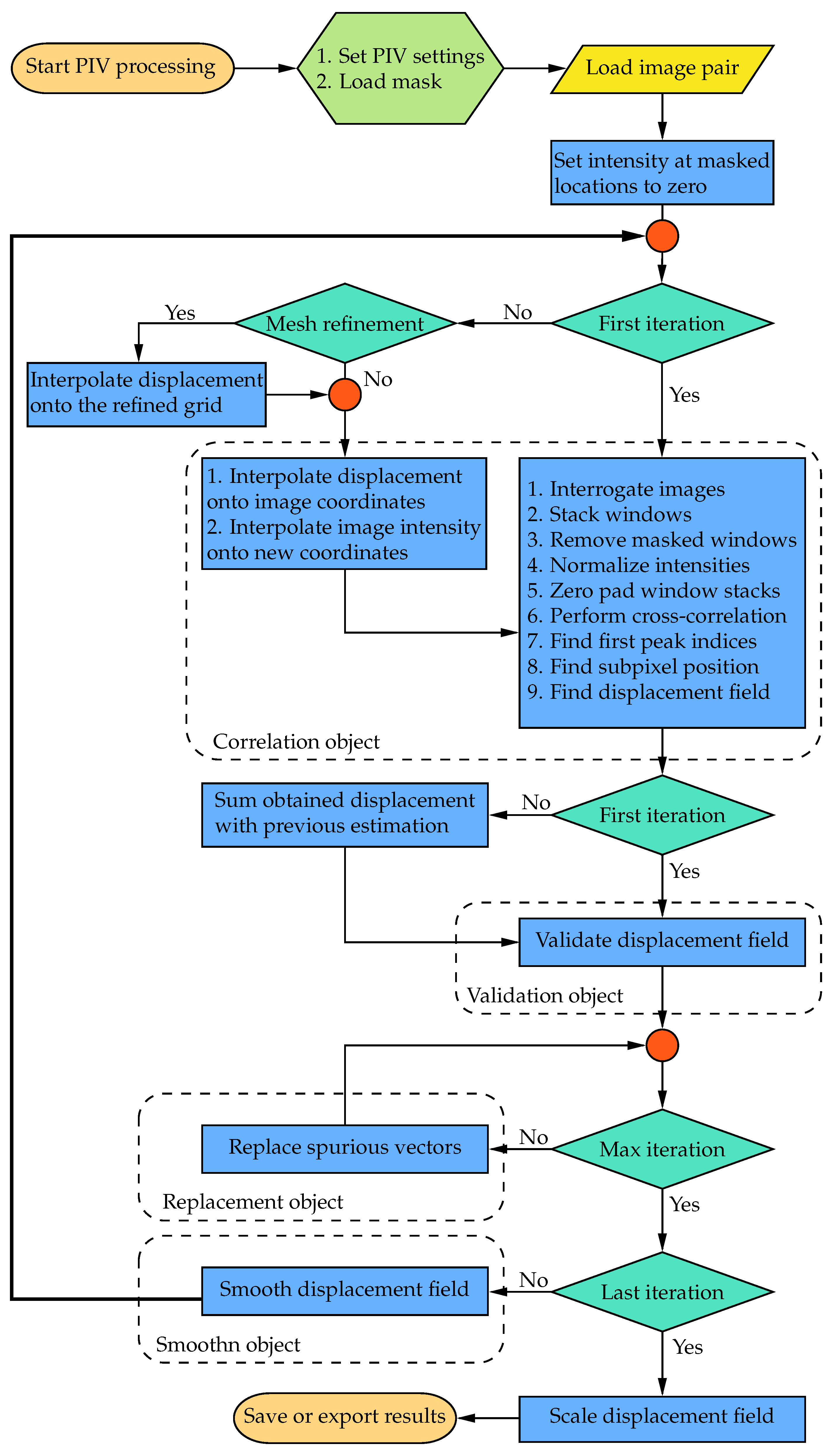
2.1. Implementation and Architecture

OpenPIV–Python was initially developed as a Python package available on the Python Package Index (PyPI). Figure 1 illustrates a flowchart detailing the typical PIV process using the WIDIM approach in the current implementation. The readers are referred to Scarano [19] for a more detailed explanation of the WIDIM algorithm. The functionalities of the original software can be categorized into four main groups: correlation, validation, replacement, and smoothing. The following sections will elaborate on the detailed enhancements made to each of these tasks, excluding smoothing, as the algorithm remains consistent with the one utilized in PIVLab and previous versions of OpenPIV [8,20].

The numerical cross-correlation process begins by dividing a pair of images into square regions, known as interrogation windows, as shown in Figure 2a. In Python, striding is applied to create two 3D stacks of all the interrogation windows for an image pair, as working with 1D arrays is more efficient for future operations, such as removing masked windows. Similarly to PIVLab, a discrete Fourier transform (DFT) is used to perform a circular cross-correlation of the two 3D arrays. The mean intensity from each window may then be subtracted as typical image data include some noisy, non-zero background signal. An important assumption in circular cross-correlation is the periodicity of the signal (image data), which may introduce frequencies in the DFT spectrum that are non-existent [2]. To suppress this negative effect, the window stacks can be zero-padded, yielding an approximation of a linear non-periodic cross-correlation [10]:

$$W_{FFT}=n_{FFT}\times W$$

(1)

where W is the window size and $W_{FFT}$ is the width of the Fourier transform. The cross-correlation is then calculated according to the cross-correlation theorem, using the Fastest Fourier Transform in the West (FFTW) available as pyFFTW on PyPI [21]. The Fourier transform width must be a power of two when using FFTW for performance reasons.

Once the cross-correlation map is calculated, the subpixel peak location may be approximated, typically using a Gaussian estimation:

$$\begin{array}{cc}\hfill i_{sp}& =i+0.5\frac{log{I}_{i-1,j}-log{I}_{i+1,j}}{log{I}_{i-1,j}-2log{I}_{i,j}+log{I}_{i+1,j}}\hfill \end{array}$$

(2a)

$$\begin{array}{cc}\hfill j_{sp}& =j+0.5\frac{log{I}_{i,j-1}-log{I}_{i,j+1}}{log{I}_{i,j-1}-2log{I}_{i,j}+log{I}_{i,j+1}}\hfill \end{array}$$

(2b)

where i and j are the peak location indices, $I_{i,j}$ denotes the value of the cross-correlation map corresponding to i and j indices, and $i_{sp}$ and $j_{sp}$ are the subpixel approximations. The displacement is then obtained by centering the subpixel peak locations using Equations (3a) and (3b) below. Note that from Equations (2a) and (2b) it is clear that no subpixel location may be estimated if the peak location is one of the borders of the correlation map. In such cases, the software uses the original peak indices to calculate the displacement.

$$\begin{array}{cc}\hfill u& =j_{sp}-\frac{W_{FFT}}{2}\hfill \end{array}$$

(3a)

$$\begin{array}{cc}\hfill v& =i_{sp}-\frac{W_{FFT}}{2}\hfill \end{array}$$

(3b)

After each iteration, the displacement field must be validated for spurious vectors to ensure the accuracy of the displacement field used as a predictor to shift and deform the interrogation windows in the next iteration. Various validation schemes have been implemented in OpenPIV [8]. The signal-to-noise ratio is a correlation-based validation method defined as the ratio of the first and second highest peaks ($I_1$ and $I_2$) in the correlation map, as shown in Equation (4) below:

$$\frac{I_1}{I_2}>{ϵ}_{S2N}$$

(4)

where ${ϵ}_{S2N}$ is the tolerance parameter, which is generally greater than 1.3 [8]. Note that it may not be feasible to use a single signal-to-noise tolerance value for all iterations as the signal-to-noise ratio decreases with every grid refinement.

Displacement-based validation methods provide a more robust alternative to the signal-to-noise ratio. Figure 2b and Figure 3a show the measurement nodes and kernels used during a typical displacement-based validation process. As shown in Figure 2b, the displacement field is padded before being stridden to create a 3D array of all kernels. The center of every kernel is then evaluated against some statistics, such as mean, median, or median absolute deviations, of its neighbors:

$$\begin{array}{cc}\hfill u_0-u_m& >r_{m,u}\times ϵ\hfill \end{array}$$

(5a)

$$\begin{array}{cc}\hfill v_0-v_m& >r_{m,v}\times ϵ\hfill \end{array}$$

(5b)

In Equations (5a) and (5b), $u_0$ and $v_0$ are the displacements at the center of the kernel while $ϵ$ is the tolerance parameter. For a simple median or mean validation, $u_m$ and $v_m$ are the median or mean of the neighbors, and $r_{m,u}=r_{m,v}=1$. For the median-absolute-deviation test, however, $u_m$ and $v_m$ are the median while $r_{m,u}$ and $r_{m,v}$ are the median absolute deviation of the neighbors. The median and median-absolute-deviation validation methods have shown to be less sensitive to the variation in vectors during the PIV process. Westerweel and Scarano [22] argued that it is possible to apply a single tolerance value for all iterations in certain scenarios.

The outliers detected during the validation process must be replaced properly to ensure the accuracy of the final displacement field or to improve the displacement field used as a predictor for the next PIV iteration. The methods implemented in the previous versions of OpenPIV replace an outlier with the mean or median of its non-spurious neighbors iteratively until the maximum number of iterations is reached. The median and mean replacement methods fail to replace the vectors that are entirely surrounded by outliers. Such vectors may be replaced in the remaining replacement iterations if a large enough number of iterations are used for the information to spread to their neighbors. In the above-described method, it is also possible to revalidate the field after each replacement iteration to exclude the outliers from the next replacement iteration when they satisfy the validation criteria. The current software allows the mean and median methods to be used with or without the revalidation option.

PIVLab, on the other hand, uses a spring analogy to replace the outliers altogether. A schematic of a system of springs is shown in Figure 3b. In this method, all measurement nodes are treated as forces applied to the ends of a spring and the outliers are replaced by solving a system of inter-connected springs with zero net force. If there are no neighboring outliers, the outlier is simply replaced by the mean of four of its neighbors. Otherwise, the method uses all of the nodes surrounding a region of outliers to interpolate the nodes within. For a displacement field with n outliers, the force balance at each node may be expressed by Equations (6a) and (6b):

$$\begin{array}{c}{x}_i-\frac{1}{a_i}\sum _{j=1}^n{\kappa }_{ij}{x}_j=\frac{1}{a_i}\sum _{k=1}^{c_i}{b}_{ik}\end{array}$$

(6a)

$$\begin{array}{c}{c}_i=a_i-\sum _{j=1}^n{\kappa }_{ij}\end{array}$$

(6b)

where an outlier and a node connected to the outlier are denoted by $x_i$ and $b_{ik}$, respectively. In Equation (6a), ${\kappa }_{ij}=1$ if an outlier is connected to the other end of one of the four springs shown in Figure 3b and zero otherwise (note that by this definition ${\kappa }_{ii}=0$ and ${\kappa }_{ij}={\kappa }_{ji}$). The coefficient $a_i$ is the number of available springs at a given node. For instance, there are only three free springs in Figure 3b since one is connected to a padded node. Generally, $a_i=3$ if a node is at the edge, $a_i=2$ if a node is in the corner, and $a_i=4$ if a node is not on the borders.

Theoretically, in the spring analogy, all of the outliers need not be replaced at once, and only the linked nodes need to be solved together, simplifying the original problem to a set of smaller systems. Hence, Equations (6a) and (6b) form multiple linear equations systems, which may be solved either separately or simultaneously. For simplicity, however, the algorithm used in the present software constructs a system of all equations before solving the system using linear algebra. Equations (6a) and (6b) may be rewritten in matrix form suitable for numerical computations:

$$\begin{array}{c}LX=B\\ L=\left[\begin{array}{cccc}1& {\displaystyle \frac{-{\kappa }_{12}}{a_1}}& \cdots & {\displaystyle \frac{-{\kappa }_{1n}}{a_1}}\\ {\displaystyle \frac{-{\kappa }_{21}}{a_2}}& 1& & {\displaystyle \frac{-{\kappa }_{2n}}{a_2}}\\ ⋮& ⋮& \ddots & ⋮\\ {\displaystyle \frac{-{\kappa }_{n1}}{a_n}}& {\displaystyle \frac{-{\kappa }_{n2}}{a_n}}& \cdots & 1\end{array}\right]\end{array}$$

(7)

In Equation (7), L and B are the linkage and coefficient matrices, respectively. Since every outlier is at most connected to four other outliers, the linkage matrix is sparse. The linkage matrix is constructed row by row using a row-based list of lists (LIL) sparse matrix before being converted into a compressed sparse row (CSR) format. In every loop, an array of zeros with the same shape as the padded displacement field is initialized, and the linkage kernel is placed at the outlier location, filling the coefficients of the connecting nodes. The row of the linkage matrix is then filled by selecting all elements corresponding to outlier locations from this array. This procedure is illustrated in Figure 4 for the first outlier in the corner ($a_1=2$) for the same field shown in Figure 2b.

The construction of the coefficient matrix in Equation (7) is straightforward. First, all elements corresponding to outlier locations in the padded field are replaced with zeros. The resulting field is stridden into a 3D array of kernels and the kernels centered around all outliers are selected from this array before calculating the mean of the nodes connected to the center of kernels. An example of this procedure for the field shown in Figure 4 is presented in Figure 5.

The remaining subroutines are described as follows. If the window size in the next PIV iteration is reduced, the filtered and smoothed displacement field is interpolated onto the new grid through bicubic interpolation. The displacement field is then interpolated onto all image coordinates using spline interpolation to build a predictor displacement field over all the image pixels. The two images are deformed according to the predictor spatial distribution. For performance reasons, the resampling of the pixel values at intermediate locations is only completed through bilinear interpolation. The deformed images are then used as input for the next iteration.

2.2. Datasets and Image Processing

Synthetic images generated from a known distribution are often used to assess the accuracy of PIV software. Synthetic images are also useful for analyzing the influence of image parameters, such as noise, particle size, or loss of particle pairs, on the performance of PIV software. Consider the turbulent flow through a rectangular channel slice of a half-height h. A Cartesian coordinate system is employed with the origin at the junction of the entrance cross-section, bottom wall, and the midspan plane, as sketched in Figure 6a.

The velocities in the x and y coordinate directions are denoted by u and v, respectively. The velocity field in the x-y plane is denoted by $\overrightarrow{v}$ and its magnitude is given by Equation (8):

$$|\overrightarrow{v}|=\sqrt{u^2+v^2}$$

(8)

since the z component of the velocity is not of interest. All time-averaged velocities are denoted by their corresponding capital letters. John Hopkins turbulent channel database contains the direct numerical simulation (DNS) results for wall-bounded turbulent flow in a rectangular channel [23]. The DNS domain size is $8\pi \times 2\times 2\pi$ using $2048\times 512\times 1536$ nodes in the x, y, and z coordinate directions, respectively. The results were obtained by solving incompressible Navier–Stokes equations with periodic boundary conditions in the stream–wise and span–wise directions and a no-slip condition at the top and bottom boundaries. The DNS grid spacing was uniform in the stream–wise direction and non-uniform in the wall-normal direction with a higher density of nodes near the wall boundary. The database contains velocity fields for 4000 simulation time steps, corresponding to approximately one flow-through period of the channel. The fluid kinematic viscosity and the friction velocity were $\nu =5\times {10}^{-5}$ and $u_{\tau }=0.0499$, corresponding to a friction velocity Reynolds number of $R{e}_{\tau }=u_{\tau }\times h/\nu \approx 1000$.

In the present study, synthetic images generated from a $2\pi \times 2$ slice of the velocity fields at $z=\pi /10$ for 1000 time steps (amounting to 2000 images) were used to assess the performance of the software to realistic and complicated flow fields. The DNS velocity field was uniformly scaled for a maximum particle displacement of 8 pixels when generating the images, satisfying the one-quarter rule for a 32 pixel × 32 pixel initial interrogation window. This corresponds to adjusting the time delay between image pairs to best capture the flow dynamics when capturing real PIV images. The synthetic images are 1608 pixels × 512 pixels large and have the same aspect ratio as the channel slice. Samples of the synthetic images of the tracer particles in the channel slice and a 32 pixel × 32 pixel window are shown in Figure 6b.

The images were processed on a workstation and the Niagara computer cluster to ensure compatibility with both the Microsoft Windows and Linux platforms and evaluate computational performance. The workstation had a 12-core Intel^® Core^™ i5-10600K CPU (Intel Corporation, Santa Clara, CA, USA) at $4.1$ GHz and 64 GB of RAM. On the Niagara cluster, a node with 40 Intel^® Skylake cores at $2.4$ GHz and 188 GB of RAM was used for PIV processing. All 1000 image pairs had to be transferred to the cluster using Globus. A list of the software input parameters and PIV settings is presented in

Table 1. Summary of PIV parameters for turbulent channel flow.

Settings	Variable	Description	Value
Masking	mask	2D array with non-zero values indicating the masked locations.	None
Data type	dtype_f 1	Type of floating-point numbers.	“float32”
Geometry	frame_shape	Size of the images.	(512, 1608)
	min_search_size	Interrogation window size for the final iteration.	8
	search_size_iters	Number of iterations for each window size.	(1, 1, 2)
	overlap_ratio	Ratio of overlap for each window size.	0.5
	shrink_ratio 2	Ratio to shrink the search size for the first iteration.	1
Correlation	deforming_order	Order of spline interpolation for window deformation.	2
	normalize	Normalize the window intensity by subtracting the mean value.	True
	subpixel_method 3	Method to estimate subpixel location of the correlation peak.	“gaussian”
	n_fft	Size factor for the 2D FFT.	(1, 1, 2)
	deforming_par 4	Ratio of the predictor used to deform each frame.	0.5
	batch_size	Batch size for calculating the cross-correlation.	1
Validation	s2n_method 5	Method of signal-to-noise ratio measurement.	“peak2peak”
	s2n_size	Half-size of a square around the first peak ignored for second peak.	2
	validation_size 6	Size parameter for validation kernel.	1
	s2n_tol 7	Tolerance for signal-to-noise ratio validation.	None
	median_tol 7	Tolerance for median validation.	2
	mad_tol 7	Tolerance for median-absolute-deviation validation.	None
	mean_tol 7	Tolerance for mean validation.	None
	rms_tol 7	Tolerance for root mean squared validation.	None
Replacement	num_replacing_iters	Number of iterations per replacement cycle.	2
	replacing_method 8	Method to use for outlier replacement.	“spring”
	replacing_size 6	Size parameter for replacement kernel.	1
	revalidate	Revalidate the fields in between replacement iterations.	True
Smoothing	smooth 9	Smooth the displacement fields.	True
	smoothing_par 10	Smoothing parameter to apply to the velocity fields.	None
Scaling	dt 11	Time delay separating the two images.	1
	scaling_par 11	Scaling factor to apply to the velocity fields.	1

¹ The available types are “float32” and “float64” for single and double floating points, respectively. ² Shrinking the window size allows for performing an extended search area PIV for the first iteration. ³ The available methods are “gaussian”, “centroid”, and “parabolic”. ⁴ A value of 0.5 corresponds to the central difference interrogation (CDI) scheme, minimizing the bias error [7]. 5 The available methods are “peak2peak”, “peak2mean”, and “peak2energy”. ⁶ The actual kernel size is obtained by kernel_size = 2 size + 1. ⁷ By selecting None, a validation method method may be ignored. ⁸ The available methods are “spring”, “mean”, and “median”. ⁹ No smoothing is applied at the end of the final iteration. ¹⁰ By selecting None, the generalized cross-validation (GCV) method is used to obtain the optimum value. ¹¹ If no scaling is applied, the output values will be in units of pixels/s.

.

The Rankine vortex is a useful case study to investigate the effects of the PIV parameters shown in Table 1 on the accuracy and performance of the software. The Rankine vortex and the adopted coordinate system are shown in Figure 7a.

The velocity field and its components in the x and y coordinate directions are denoted by $\overrightarrow{v}$, u, and v, respectively. The velocity magnitude and its distribution for the Rankine vortex are given by Equations (8) and (9):

$$\left\{\begin{array}{cc}|\overrightarrow{v}|=\frac{r}{R}{\left|\overrightarrow{v}\right|}_R\hfill & r<R\hfill \\ \overrightarrow{v}=\frac{R}{r}{\left|\overrightarrow{v}\right|}_R\hfill & r⩾R\hfill \end{array}\right.$$

(9)

where r is the distance from the vortex center, R is the radius of the vortex core, and ${\left|\overrightarrow{v}\right|}_R$ is the velocity magnitude at $r=R$. A pair of synthetic images of the size $512 \mathrm{pixels}\times 512 \mathrm{pixels}$ were generated from the Rankine vortex distribution using PIVLab. The vortex core was located at the center of the frame and had a radius of $R=50 \mathrm{pixels}$. The number of particles, particle diameter, and noise level were set to 50,000, 3 $\mathrm{pixels}$, and 0.001, respectively. The maximum particle velocity was scaled to $|\overrightarrow{v}{|}_R=16 \mathrm{pixels}/\mathrm{s}$ to satisfy the one-quarter rule for a $64 \mathrm{pixels}\times 64 \mathrm{pixels}$ initial interrogation window. A sample of these images is shown in Figure 7b.

3. Results

In this section, contour plots, vector plots, and one-dimensional profiles are presented to evaluate the accuracy of the algorithms in resolving the instantaneous and time-averaged flow characteristics. Python was used to calculate the average of 1000 velocity fields for both the DNS and PIV results. The velocity and displacement throughout the rest of this paper are in units of $\mathrm{pixels}$/$\mathrm{s}$ and $\mathrm{pixels}$, respectively. All data visualizations were accomplished using the commercial software Origin^®.

3.1. Mean Flow Field

Figure 8 compares the contour plots of the mean stream–wise velocity for the DNS data and PIV results. From Figure 8a,b, it can be seen that the OpenPIV results captured all of the major patterns found in the contour plot of the DNS data, and closely matched all the large-scale contour lines. The discrepancies found between Figure 8a,b are mostly concentrated near the bottom and top walls, near the entrance and exit cross-sections, and in high-velocity regions.

The one-dimensional profiles of the mean stream–wise velocity are provided in Figure 9 to better visualize the stream–wise evolution of the flow. The profiles were plotted at five successive stream–wise locations, starting at $x=4$ and ending at $x=1604$ with an increment of 400, allowing the DNS data and PIV results to be compared in both near boundary and internal regions. In the near-wall regions, the small-scale structures are averaged out from the DNS data during the generation of the images [8,24]. The wall coordinates are defined as follows:

$$y^{+}=\frac{u_{\tau }\Delta y}{\nu }$$

(10)

The PIV measurement nodes closest to the bottom and top walls are located at $y=4$ and $y=508$, corresponding to $y^{+}\approx 16$ (given that $R{e}_{\tau }\approx 1000$). Since these nodes are near the edge of the shear layers, their values are biased towards the larger velocities, which may also be observed in Figure 9.

The disparity between the DNS data and the PIV results at the entrance and exit cross-sections ($x=4$ and $x=1604$) occurs due to the loss of particle pairs that cannot be redeemed by window translations and deformation. For a given image pair, the particles entering or leaving the frame are only present in one of the two images, leading to a significant loss of correlation. The current software tends to remedy this negative effect using bilinear extrapolation to resample the image intensity near the boundaries. In general, it is good practice to discard at least the layer immediately near the borders of the velocity fields.

Figure 10 shows the frequency distribution plots of the error (difference between the DNS and PIV results) for the mean velocity magnitude, mean stream–wise velocity, and the mean transverse velocity. The sample size, mean, and standard deviation of the velocity magnitude error were 50,927, 0.003, and 0.116, respectively. These results, as well as the 95% confidence intervals shown in Figure 10a–c, indicate that the software is capable of resolving all time-averaged velocities with reasonable accuracy.

3.2. Instantaneous Flow Field

The performance of the software in resolving the instantaneous flow field was evaluated by analyzing the fluctuating velocities, span–wise vorticity, and Q-criterion. The fluctuating velocities and the span–wise vorticity are given by Equations (11a) and (11b):

$$\begin{array}{cc}\hfill u^{\prime }& =u-U\hfill \end{array}$$

(11a)

$$\begin{array}{cc}\hfill v^{\prime }& =v-V\hfill \end{array}$$

(11b)

The coherent structures in the flow can be identified using the Q-criterion. The Q-criterion is a scalar field that defines structures as regions where the vorticity magnitude is greater than the magnitude of the strain rate. In a two-dimensional Cartesian coordinate system, the Q-criterion is given by Equation (12) below:

$$Q=-\frac{1}{2}\left({\left(\frac{\partial u}{\partial x}\right)}^2+2\left(\frac{\partial u}{\partial y}\right)\left(\frac{\partial v}{\partial x}\right)+{\left(\frac{\partial v}{\partial y}\right)}^2\right)$$

(12)

In the present study, the instantaneous velocity gradients were calculated using second-order accurate central differences in the interior points and first-order accurate one-side differences at the boundaries to calculate Equation (12). The fluctuating velocity vectors superimposed on top of the contour plots of the Q-criterion for the DNS data and PIV results at an arbitrary time step are presented in Figure 11.

In both Figure 11a,b, the Q-criterion was normalized by its maximum value in the DNS data. The main structures in the DNS data are also captured in the PIV results. In the middle section of the channel where the velocity is large, small isolated regions of negative Q values are present in the PIV results, which may not be seen in the DNS data. Many of these regions, a few of which are marked with red circles in Figure 11b, corresponded to the vectors that were replaced during the last iteration, indicating the effectiveness of the median validation in detecting the outliers. It is important to note that the median validation did not classify these vectors as outliers at the end of the process. These vectors, nevertheless, are approximated from their neighbors and should be regarded as unreliable.

The density of the vector field may be increased by means of decreasing the minimum window size or increasing the final overlap. The same vector spacing of 4 $\mathrm{pixels}$ may be achieved by setting only min_search_size=16 and overlap_ratio=(0.5, 0.5, 0.75) from the parameters in Table 1. This will significantly improve the results away from the walls ($100<y<400$) and at the entrance and exit cross-sections. Obviously, the near-wall results will not be as detailed when a larger min_search_size is used. These results are provided as supplementary figures in Appendix B.

Figure 12 shows the frequency distribution plots of the error for the velocity magnitude, stream–wise velocity, and transverse velocity to further assess the accuracy of the instantaneous velocity fields. The sample size, mean, and standard deviation of the velocity magnitude error were 50,927,000, 0.005, and 0.208, respectively. In Figure 12a–c, the 95% confidence interval is specified by two dashed vertical lines. These confidence intervals may be significantly improved if the boundary nodes are discarded. The results show that the software is capable of resolving the instantaneous velocities with reasonable accuracy.

3.3. Computational Performance

Figure 13 demonstrates the effect of the number of processors on the computation time. Multiprocessing was employed to vary the number of utilized processors for both the workstation and Niagara cluster. Initially, for both platforms, the computation time decreases rapidly as more processors are utilized. Meanwhile, launching more processes above a certain threshold did not impact the calculation time. The time needed to transfer 2000 images to the Niagara cluster using Globus was 863 s at an effect speed of $3.81$ MB/s. From Figure 13, it can be seen that the speedup achieved by using the Niagara cluster is not enough to compensate for the data transfer time. Using the cluster only becomes sensible when large images with computationally intensive settings are to be processed or when a dataset needs to be processed more than once.

CPU–Based PIV software, unlike their GPU counterparts, generally should cycle through the windows rather than performing the cross-correlation simultaneously. Hence, it is recommended always to set batch_size=1 for optimum performance. Regardless of whether the cross-correlation is parallelized or not, the most time-consuming calculation in a PIV algorithm is generally computing the cross-correlation between the interrogation windows. The relative computational time for most of the sub-routines is presented in Figure 1 is reported in

Table 2. Performance profile of the CPU–Based software.

Subroutine	Computational Time per Run 1					Average
Interrogation	0.893	0.894	0.833	0.867	0.791	0.855
Deformation 2	14.596	14.533	14.626	14.308	4.511	14.515
Normalization	1.902	1.865	1.783	1.852	1.820	1.845
Cross-correlation	65.573	65.769	65.797	66.103	65.560	65.760
Peak estimation 3	1.203	1.282	1.190	1.222	1.263	1.232
Validation	3.066	3.185	3.209	3.153	3.124	3.148
Replacement	3.493	3.615	3.727	3.587	3.639	3.612
Smoothing	0.658	0.698	0.672	0.748	0.671	0.689
Time per vector 4	50.611	50.557	49.586	49.859	49.704	50.063

¹ For the subroutines, the reported values are the percentage of the relative computational time defined as the time required for the subroutine divided by the total processing time. ² Deformation refers to the combination of window and frame deformation. ³ Peak estimation refers to the process of finding the first peak and estimating its subpixel location. ⁴ Computational time per vector is presented in units of μs and is obtained as the total calculation time divided by the number of vectors in the resulting vector field.

. The relative computational time was calculated five times using the same parameters shown in Table 1 before being averaged. As expected, cross-correlation was the most time-consuming subroutine with nearly 65% of the total computation time. Although deformation is the second most time-consuming subroutine, it is worth mentioning that a larger portion of the time is spent on frame deformation. Since window deformation is not as time-consuming, using a deforming_order greater than one is recommended for better accuracy. Overall, 84.207% of the calculation time was spent in the correlation object, which handles the main PIV calculations, while only 7.449% of the time was dedicated to validation, replacement, and smoothing altogether, further indicating that the software is implemented well.

4. Discussion

The effect of several PIV parameters, including data type, number of PIV iterations, correlation width, number of replacement iterations, replacing method, and revalidation, on the Rankine vortex dataset described in Section 2 are discussed in this section. The readers are referred to Meunier and Leweke [7] for a detailed discussion on the effect of the deformation parameter on the bias error. For each case study, all parameters are the same as in Table 1 with the exception of the parameters being investigated, frame_shape=(512, 512) and min_search_size=16. After the effect of the PIV parameters on the resulting field is discussed, a comparison between the results derived using the best replacement method and PIVLab results obtained using the same number of iterations with a minimum window size of 16 $\mathrm{pixels}$ is presented.

The precision of the floating-point data used during the PIV process can significantly impact the computational performance. Although both single and double precisions are available options, the single precision data type is preferred as it can greatly reduce the cross-correlation computation time. Performing the PIV analysis for both double and single data types resulted in the same mean, standard deviation, and 95% confidence interval of $-0.061$, $0.374$, and $(-0.984, 0.204)$ for the velocity magnitude error. In general, using the single precision data type should not be a problem for most PIV applications.

The number of iterations used at each window size may remarkably improve the accuracy of the results. For instance, just performing one more iteration for the $32 \mathrm{pixels}\times 32 \mathrm{pixels}$ window size, that is, changing search_size_iters=(1, 1, 2) to (1, 2, 2), can change the 95% confidence interval of the velocity magnitude error from $(-0.984, 0.204)$ to $(-0.657, 0.211)$.

As was discussed in Section 2, zero-padding the windows before taking the circular-cross correlation may improve the results. It is recommended to increase the correlation width for the minimum window size at least by a factor of two to strike a balance between accuracy and computation efficiency. Increasing the correlation width for other window sizes, although not as effective as the smallest window size, may also improve the accuracy. For example, changing n_fft=(1, 1, 2) to (1, 2, 2) reduces the 95% confidence interval of the velocity magnitude error from $(-0.984, 0.204)$ to $(-0.805, 0.203)$.

The number of replacement iterations can become an important PIV parameter depending on the replacement method. For the spring replacement method, using one iteration is sufficient since this method replaces the outliers altogether. There is no rule to determine the number of iterations required for the convergence of the mean and median methods. It may take several iterations for these methods to converge if revalidation is not applied depending on the number of outliers and their connection. For this case study, the mean and median methods converged after three iterations when the fields were revalidated. Without revalidation, on the other hand, it took 16 and 34 iterations for the mean and median methods to converge, respectively.

The effect of the replacement method on the accuracy of the results is not straightforward. Replacing outliers with reasonable estimations increases the chance of obtaining a better correlation match in the subsequent PIV iterations. The outliers replaced during the last iteration, however, are not reliable since all of the replaced vectors are simply approximated from their neighbors. Figure 14 shows the exact velocity field and the results obtained with three replacement methods. The mean and median replacements were performed using five iterations to reach convergence. The green vectors indicate the outliers that were replaced during the last iteration and satisfied the validation criteria at the end of the process. The remaining outliers are designated in red color and amounted to three, one, and, two for spring, mean, and median methods, as can be seen in Figure 14a–c, respectively.

The mean, standard deviation (STD), and 95% confidence interval (95% CI) of the velocity components and velocity magnitude are reported in

Table 3. Mean, standard deviation, and 95% confidence interval of velocity errors for different replacement methods.

Method	Error	Mean	STD 1	95% CI 2
Spring	u	$-0.011$	$0.356$	$(-0.645, 0.480)$
	v	$0.004$	$0.419$	$(-0.593, 0.582)$
	$|\overrightarrow{v}|$	$-0.073$	$0.438$	$(-1.231, 0.217)$
Mean	u	$-0.005$	$0.345$	$(-0.569, 0.521)$
	v	$-0.007$	$0.303$	$(-0.544, 0.521)$
	$|\overrightarrow{v}|$	$-0.045$	$0.301$	$(-0.732, 0.196)$
Median	u	$-0.002$	$0.378$	$(-0.620, 0.504)$
	v	$0.001$	$0.374$	$(-0.541, 0.597)$
	$|\overrightarrow{v}|$	$-0.053$	$0.346$	$(-0.783, 0.210)$

¹ Standard deviation. ² 95% confidence interval.

. It can be seen that all values in Table 3 are of the same order of magnitude. For this particular set of parameters, the mean method yielded the minimum mean absolute error (MAE) and root mean squared error (RMSE) of 0.303 and 0.459, respectively.

The effect of revalidation on the results obtained with the mean and median replacement methods is shown in Figure 15. Although revalidation always reduces the number of iterations needed for convergence, it does not necessarily improve the accuracy of the results. By comparing Figure 15a with Figure 15b and Figure 15c with Figure 15d, it can be seen that revalidation has improved the results only for the mean method. The mean replacement with revalidation performed the best since fewer vectors were replaced during the last PIV iteration and only one outlier remains after the process. For the best practice, it is recommended to perform a few pilot runs before PIV analysis to decide on the replacement and validation options, aiming to minimize the replaced vectors during the last PIV iteration. Note that revalidation is not applicable to the signal-to-noise ratio validation method since the signal-to-noise ratio is correlation-based and is not affected by the replaced vectors.

A comparison of the results of the developed software, obtained using the mean replacement methods with revalidation, and the PIVLab results is shown in Figure 16. Note that no post-processing was applied to the PIVLab results. PIVLab provides utilities for velocity-based and image-based validation during the post-processing steps. The vector field shown in Figure 16 is what is obtained solely using the validation and smoothing routines in between the PIV iterations. From Figure 16, it is clear that with the exception of one vector at $(x,y)=(352, 32)$, the remaining different vectors are focused near the center of the vortex. Using the local median filter with a threshold of two, the post-processing step in PIVLab showed that this vector is an outlier. Using the present software, however, this vector was reliably obtained using cross-correlation. More such instances were identified among the outliers near the center of the vortex. Although PIVLab allows for replacement of the remaining outliers using interpolation, the vectors replaced during the post-processing phase or the last PIV iteration are not reliable, as was confirmed by the DNS data.

5. Conclusions

An open-source CPU–Based PIV data processing software was developed and validated. The software was written entirely in Python and was compatible with the Microsoft Windows and Linux operating systems. The software was functional on different hardware platforms, ranging from small embedded systems to large supercomputing clusters. Synthetic PIV images generated from the John Hopkins turbulent rectangular channel DNS data were processed to test the accuracy of the software in resolving the mean and instantaneous flow fields and computation performance.

Both the mean and instantaneous velocities closely matched the DNS data except near the walls, where the lengths scales are much smaller than the smallest PIV interrogation window, near the entrance and exit cross-sections, and in high-velocity regions. Isolated regions of low Q-criterion values were detected in the PIV results, which were not observed in the DNS data. Further investigations showed that such discrepancies in high-velocity regions may be avoided by using a larger window size for the final iteration. These analyses showed that the vectors replaced during the last iteration, even when they are not detected as outliers after the PIV process, must be marked as unreliable.

The computational performance of the software was evaluated on a workstation and the Niagara cluster. For both cases, the computation time initially decreased significantly as more processors were used. Meanwhile, the profiles almost remained flat once enough processors were utilized. The relative computation times of different subroutines of the software were measured during five runs and averaged to obtain the performance profile. The cross-correlation and deformation subroutines constituted the major portion of the total computation time. The relative computation times for validation, replacement, and smoothing subroutines, on the other hand, were significantly lower, indicating the efficiency of the algorithms.

The effect of several PIV parameters on the output velocity field for the Rankine vortex dataset was investigated. Using a double precision floating-point data did not affect the quality of the results. Using more PIV iteration or zero-padding the correlation generally tends to improve the accuracy. The errors associated with using different replacement methods were all of the same order of magnitude. Revalidation was shown to be effective in reducing the number of iterations needed for convergence of the resulting fields. Finally, the velocity field obtained with the best set of the discussed parameters showed good agreement with the PIVLab results. The discrepancies between the results of the two software were mostly confined to a few vectors near the center of the vortex.

Overall, the present study showed that the developed software is accurate and computationally efficient, and can be reliably used on the Microsoft Windows and Linux platforms to process large datasets. The software was tested on a standard computer workstation, a CPU cluster, and Google Colaboratory cloud computing service as part of this study. Hence, the software could be run on computer clusters or cloud computing services to avoid investing in hardware or needing affiliation with a university. The software offers great flexibility, enabling the users to adjust the settings according to their needs. Although the parameters were tuned to obtain more accurate results throughout this paper, it is also possible to adjust the parameters for fast PIV processing at the cost of accuracy.

References

1. Adrian, R.J. Twenty years of particle image velocimetry. Exp. Fluids 2005, 39, 159–169. [Google Scholar] [CrossRef]
2. Raffel, M.; Willert, C.E.; Scarano, F.; Kähler, C.J.; Wereley, S.T.; Kompenhans, J. Particle Image Velocimetry: A Practical Guide, 3rd ed.; Springer International: Cham, Switzerland, 2018. [Google Scholar] [CrossRef]
3. Booth-Gauthier, E.A.; Alcoser, T.A.; Yang, G.; Dahl, K.N. Force-induced changes in subnuclear movement and rheology. Biophys. J. 2012, 103, 2423–2431. [Google Scholar] [CrossRef] [PubMed]
4. Sarno, L.; Carravetta, A.; Tai, Y.C.; Martino, R.; Papa, M.; Kuo, C.Y. Measuring the velocity fields of granular flows–Employment of a multi-pass two-dimensional particle image velocimetry (2D-PIV) approach. Adv. Powder Technol. 2018, 29, 3107–3123. [Google Scholar] [CrossRef]
5. Voorneveld, J.; Kruizinga, P.; Vos, H.J.; Gijsen, F.J.; Jebbink, E.G.; Van Der Steen, A.F.; De Jong, N.; Bosch, J.G. Native blood speckle vs ultrasound contrast agent for particle image velocimetry with ultrafast ultrasound-in vitro experiments. In Proceedings of the 2016 IEEE International Ultrasonics Symposium (IUS), Tours, France, 18–21 September 2016; pp. 1–4. [Google Scholar] [CrossRef]
6. Scarano, F.; Riethmuller, M.L. Iterative multigrid approach in PIV image processing with discrete window offset. Exp. Fluids 1999, 26, 513–523. [Google Scholar] [CrossRef]
7. Meunier, P.; Leweke, T. Analysis and treatment of errors due to high velocity gradients in particle image velocimetry. Exp. Fluids 2003, 35, 408–421. [Google Scholar] [CrossRef]
8. Dallas, C.; Wu, M.; Chou, V.; Liberzon, A.; Sullivan, P.E. Graphical Processing Unit-Accelerated Open-Source Particle Image Velocimetry Software for High Performance Computing Systems. J. Fluids Eng. 2019, 141, 111401. [Google Scholar] [CrossRef]
9. Ben-Gida, H.; Gurka, R.; Liberzon, A. OpenPIV-MATLAB—An open-source software for particle image velocimetry; test case: Birds’ aerodynamics. SoftwareX 2020, 12, 100585. [Google Scholar] [CrossRef]
10. Thielicke, W.; Sonntag, R. Particle Image Velocimetry for MATLAB: Accuracy and enhanced algorithms in PIVlab. J. Open Res. Softw. 2021, 9, 12. [Google Scholar] [CrossRef]
11. PIVLab. Available online: https://www.mathworks.com/matlabcentral/fileexchange/27659-pivlab-particle-image-velocimetry-piv-tool-with-gui (accessed on 15 August 2023).
12. OpenPIV. Available online: http://www.openpiv.net/ (accessed on 15 August 2023).
13. Fluere. Available online: https://www.softpedia.com/get/Science-CAD/Fluere.shtml (accessed on 15 August 2023).
14. Fluidimage. Available online: https://pypi.org/project/fluidimage/ (accessed on 15 August 2023).
15. mpiv. Available online: https://www.mathworks.com/matlabcentral/fileexchange/2411-mpiv (accessed on 15 August 2023).
16. JPIV. Available online: https://eguvep.github.io/jpiv/ (accessed on 15 August 2023).
17. UVMAT. Available online: http://servforge.legi.grenoble-inp.fr/projects/soft-uvmat (accessed on 15 August 2023).
18. Yang, E.; Ekmekci, A.; Sullivan, P.E. Phase evolution of flow controlled by synthetic jets over NACA 0025 airfoil. J. Vis. 2022, 25, 751–765. [Google Scholar] [CrossRef]
19. Scarano, F. Iterative image deformation methods in PIV. Meas. Sci. Technol. 2001, 13, R1. [Google Scholar] [CrossRef]
20. Garcia, D. Robust smoothing of gridded data in one and higher dimensions with missing values. Comput. Stat. Data Anal. 2010, 54, 1167–1178. [Google Scholar] [CrossRef] [PubMed]
21. Gomersall, H. pyFFTW: Python Wrapper around FFTW. Astrophys. Source Code Libr. 2021, ascl:2109.009. Available online: http://xxx.lanl.gov/abs/2109.009 (accessed on 15 August 2023).
22. Westerweel, J.; Scarano, F. Universal outlier detection for PIV data. Exp. Fluids 2005, 39, 1096–1100. [Google Scholar] [CrossRef]
23. Perlman, E.; Burns, R.; Li, Y.; Meneveau, C. Data Exploration of Turbulence Simulations Using a Database Cluster. In Proceedings of the 2007 ACM/IEEE Conference on Supercomputing, SC’07, New York, NY, USA, 10–16 November 2007. [Google Scholar] [CrossRef]
24. Saikrishnan, N.; Marusic, I.; Longmire, E.K. Assessment of dual plane PIV measurements in wall turbulence using DNS data. Exp. Fluids 2006, 41, 265–278. [Google Scholar] [CrossRef]
Figure 1. Flowchart of the architecture of OpenPIV–Python-CPU.
Fluids 08 00285 g001
Figure 2. A 512   pixels × 512   pixels synthetic image of tracer particles in a Rankine vortex: (a) interrogation windows of size 128   pixels × 128   pixels with zero overlap; (b) measurement (blue) and padded (red) nodes are shown, respectively.
Fluids 08 00285 g002
Figure 3. Schematics of a kernel of size three, showing center and neighboring nodes used during validation and replacement processes: (a) validation kernel; (b) spring analogy for outliers replacement. Measured nodes (blue), Padded nodes (red) and outliers (white) are shown.
Fluids 08 00285 g003
Figure 4. A schematic showing an array of zeros and a kernel of size three used to construct the linkage matrix. The white nodes are selected to fill the first row of the linkage matrix. Measured nodes (blue), Padded nodes (red), and outliers (white) are shown.
Fluids 08 00285 g004
Figure 5. An example showing the kernels used for constructing the right-hand side of Equation (7). Note that the gray nodes will not be used when calculating the average in each kernel.
Fluids 08 00285 g005
Figure 6. A schematic representation of the wall-bounded turbulent rectangular channel flow: (a) the adopted nomenclature; (b) a sample of the synthetic images used in the present study and tracer particles in a 32   pixels × 32   pixels window.
Fluids 08 00285 g006
Figure 7. A schematic representation of Rankine vortex: (a) the adopted nomenclature; (b) a sample of the synthetic images used in the present study.
Fluids 08 00285 g007
Figure 8. Contour plots of the mean stream–wise velocity: (a) John Hopkins DNS data; (b) results obtained with OpenPIV–Python.
Fluids 08 00285 g008
Figure 9. Stream–wise evolution of the mean stream–wise velocity profiles.
Fluids 08 00285 g009
Figure 10. Frequency distribution plots of velocity error for the mean velocity fields: (a) velocity magnitude; (b) stream–wise velocity; (c) transverse velocity. The 95% confidence interval is shown by dashed vertical lines on each plot.
Fluids 08 00285 g010
Figure 11. Vectors of the fluctuating velocities superimposed on the contour plots of the normalized Q-criterion: (a) John Hopkins DNS data; (b) results obtained with OpenPIV–Python.
Fluids 08 00285 g011
Figure 12. Frequency distribution plots of velocity error for 1000 instantaneous velocity fields: (a) velocity magnitude; (b) stream–wise velocity; (c) transverse velocity. The 95% confidence interval is shown by dashed vertical lines on each plot.
Fluids 08 00285 g012
Figure 13. Plot of the computation time against the core number.
Fluids 08 00285 g013
Figure 14. Effect of replacing methods on the velocity fields: (a) exact velocity field; (b) spring replacement; (c) mean replacement; (d) median replacement. Replaced vectors satisfying the validation criteria at the end of the final iteration are designated in green color. Any remaining outliers are represented in red color.
Fluids 08 00285 g014
Figure 15. Effect of revalidation on the velocity fields: (a) mean replacement and no revalidation; (b) mean replacement with revalidation; (c) median replacement and no revalidation; (d) median replacement with revalidation. Replaced vectors satisfying the validation criteria at the end of the final iteration are designated in green color. Any remaining outliers are represented in red color.
Fluids 08 00285 g015
Figure 16. Comparison between the results obtained with the developed software and PIVLab: (a) PIVLab original results with no further post-processing; (b) results obtained with the present software using mean replacement with revalidation.
Fluids 08 00285 g016