Radial Basis Function Surrogates for Uncertainty Quantification and Aerodynamic Shape Optimization under Uncertainties

Abstract

This paper investigates the adequacy of radial basis function (RBF)-based models as surrogates in uncertainty quantification (UQ) and CFD shape optimization; for the latter, problems with and without uncertainties are considered. In UQ, these are used to support the Monte Carlo, as well as, the non-intrusive, Gauss Quadrature and regression-based polynomial chaos expansion methods. They are applied to the flow around an isolated airfoil and a wing to quantify uncertainties associated with the constants of the $\gamma -\tilde{R}{e}_{\theta t}$ transition model and the surface roughness (in the 3D case); it is demonstrated that the use of the RBF-based surrogates leads to an up to 50% reduction in computational cost, compared with the same UQ method that uses CFD computations. In shape optimization under uncertainties, solved by stochastic search methods, RBF-based surrogates are used to compute statistical moments of the objective function. In applications with geometric uncertainties which are modeled through the Karhunen–Loève technique, the use on an RBF-based surrogate reduces the turnaround time of an evolutionary algorithm by orders of magnitude. In this type of applications, RBF networks are also used to perform mesh displacement for the perturbed geometries.

1. Introduction

Gradient-free and gradient–based optimization methods are nowadays broadly used to solve shape optimization problems in aerodynamics. The same problems may also consider uncertainties related to the boundary conditions, the flow model constants or geometric imperfections, in which cases uncertainty quantification (UQ) methods are needed. In an aerodynamic shape optimization loop, performing the UQ for any quantity of interest (QoI) significantly increases the cost, since many calls to the computational fluid dynamics (CFD) tool are needed.

Given that sampling-based techniques such as Monte Carlo (MC) are prohibitively expensive in computationally demanding problems, other efficient UQ approaches have been proposed instead. The most important among them rely upon the spectral representation of the uncertain quantities, referred to as the polynomial chaos expansion (PCE) and the method of moments (MoM). The former can be used as an either non-intrusive or intrusive technique [1,2,3,4,5,6,7]. First-Order Second-Moment, Second-Order Second-Moment as well as projected variants of the MoM [8,9,10,11] can been found in the literature.

In UQ, the trend is to replace the computationally expensive CFD tool with artificial intelligence (AI)-based surrogates. For instance, in [12], uncertainties in multi-phase CFD simulations for bubbly flows were quantified and reduced using machine learning (ML) techniques. Feed-forward neural networks and principal component analysis were used as surrogates to the multi-phase CFD model and Gaussian processes for uncertainty evaluation. The procedure was supported by experimental measurements and it was demonstrated that the proposed approach is capable of both quantifying and reducing the uncertainties in multi-phase problems. Radial Basis Function (RBF) networks were used as surrogate models in UQ of age and time-dependent fracture mechanics in [13]; emphasis was laid on the prediction of the energy release rate in a concrete plate section with the presence of an initial surface crack. The RBF models used to support MC proved to be accurate enough despite the relatively small number of patterns/samples used to train them. An AI-based smart proxy model to a multiphase CFD solver was created in [14] so as to reduce the computational cost due to the required gas–solid flow simulations. It was shown that a feed-forward artificial neural network (ANN) can accurately predict the gas–solid flow behavior in fluidized beds. In [15], a data–driven approach for modeling turbulent and transitional flows, based on inverse modeling and ML, was proposed. The aim was to quantify deficiencies in turbulence and transition modeling using data from simulations and measurements. The method was applied in turbulent (over a convex wall) and transitional (over a flat plate) flows by modeling non-equilibrium turbulent boundary layers and bypass transition. For transitional flows, in [16], UQ and sensitivity analysis was performed for the two-equation $\gamma -\tilde{R}{e}_{\theta t}$ transition model. The idea was to quantify the contribution of the model’s parameters to QoIs strongly related to transition effects such as the skin friction coefficient, the transition onset and length and the size of the separation bubble. The study was carried out for a series of flat plates and two isolated airfoils; overall, it was concluded that the parameters which affect the uncertainty of QoIs were those related to the $\gamma$ equation.

In UQ, which accounts for geometric imperfections and in aerodynamic shape optimization, the need for adapting an existing mesh to new boundaries emerges. Mesh displacement methods are nowadays frequently used instead of re-meshing. Among the various methods proposed in the literature (based on spring analogies, the solution of partial differential equations (PDEs), etc.), mesh displacement that takes advantage of RBF interpolations [17,18,19] was proved to be fast and efficient for large deformations and complex geometries.

This paper investigates and assesses the use of RBF-based surrogate evaluation models, instead of expensive CFD codes, for UQ and aerodynamic shape optimization problems with or without uncertainties. In UQ, the usage of the RBF surrogates is multifaceted as these are incorporated into three different techniques which, by their own nature, are computationally demanding as they need many calls to the evaluation software. In specific, surrogates are used to support the Monte Carlo, the Gauss Quadrature (GQ) and the regression-based PCE. It was also selected to demonstrate the capabilities of these approaches in two different kinds of problems: (a) UQ related to ambiguities regarding the proper values of the constants and surface roughness in the $\gamma -\tilde{R}{e}_{\theta t}$ transition model in Reynolds-averaged Navier–Stokes (RANS) simulations and (b) shape optimization under uncertainties, in which these are generated using the Karhunen–Loève (KL) method and the optimization is performed using a stochastic, population-based search method. In case of geometrical uncertainties, the RBF-based surrogate computes the statistical moments of the QoI; in such a case, re-meshing is avoided by using a two-step RBF-based mesh displacement method.

2. Methods and Tools

2.1. CFD Tool—Governing Equations

In this work, the CFD tool used is the GPU-accelerated in-house code PUMA [20], which solves the RANS equations for steady flows of compressible fluids. The mean-flow equations for 3D flows read

$$\frac{\partial U_n}{\partial \tau }+\frac{\partial f_{nk}^{\mathrm{inv}}}{\partial x_k}-\frac{\partial f_{nk}^{\mathrm{vis}}}{\partial x_k}=0,n\in [1,5]$$

(1)

and are solved for the conservative flow variables $U={\left[\rho \rho v_1\rho v_2\rho v_3\rho E\right]}^T$, where $\rho$ stands for the fluid’s density, $v_k$ are the Cartesian velocity components ($k\in [1,3]$), $E=\frac{p}{\gamma - 1}+\frac{1}{2}\rho v_k{v}_k$ the total energy per unit mass and p the pressure. $\tau$ is the pseudo-time step and $x_k$ the Cartesian coordinates. $f_{nk}^{\mathrm{inv}}$ are the inviscid fluxes and $f_{nk}^{\mathrm{vis}}$ the viscous ones which involve the stress tensor ${\tau }_{km}=\left(\mu +{\mu }_t\right)\left(\frac{\partial v_k}{\partial x_m}+\frac{\partial v_m}{\partial x_k}-\frac{2}{3}{\delta }_{km}\frac{\partial v_{\ell }}{\partial x_{\ell }}\right)$. Turbulence is modeled by the one-equation Spalart–Allmaras model [21], computing ($\tilde{\nu }$) by solving

$$\frac{\partial \left(\rho \tilde{\nu }\right)}{\partial \tau }+\frac{\partial \left(\rho \tilde{\nu }{v}_k\right)}{\partial x_k}-\frac{\rho }{\sigma }\left\{\frac{\partial }{\partial x_k}\left[\left(\nu +\tilde{\nu }\right)\frac{\partial \tilde{\nu }}{\partial x_k}\right]+c_{b_2}\frac{\partial \tilde{\nu }}{\partial x_k}\frac{\partial \tilde{\nu }}{\partial x_k}\right\}-{\tilde{P}}_{\tilde{\nu }}+D_{\tilde{\nu }}=0$$

(2)

and ${\mu }_t=\rho \tilde{\nu }{f}_{v1}$. The production term reads ${\tilde{P}}_{\tilde{\nu }}=\rho c_{b1}(1-f_{t2})\tilde{S}\tilde{\nu }$, while the definition of all other terms and constants can be found in [21]. To predict laminar-to-turbulent transition, the $\gamma -\tilde{R}{e}_{\theta t}$ transition model [22],

$$\begin{array}{cc}\hfill & \frac{\partial \left(\rho \gamma \right)}{\partial \tau }+\frac{\partial \left(\rho v_k\gamma \right)}{\partial x_k}-\frac{\partial }{\partial x_k}\left[\left(\mu +\frac{{\mu }_t}{{\sigma }_f}\right)\frac{\partial \gamma }{\partial x_k}\right]-P_{\gamma }+D_{\gamma }=0\hfill \end{array}$$

(3)

$$\begin{array}{cc}\hfill & \frac{\partial \left(\rho \tilde{R}{e}_{\theta t}\right)}{\partial \tau }+\frac{\partial \left(\rho v_k\tilde{R}{e}_{\theta t}\right)}{\partial x_k}-\frac{\partial }{\partial x_k}\left[{\sigma }_{\theta ,t}\left(\mu +{\mu }_t\right)\frac{\partial \tilde{R}{e}_{\theta t}}{\partial x_k}\right]-P_{\theta ,t}-D_{SCF}=0\hfill \end{array}$$

(4)

is additionally solved to compute the fields of intermittency $\gamma$ and transition momentum thickness Reynolds number $\tilde{R}{e}_{\theta t}$. The production and destruction terms in this model are

$$\begin{array}{cc}\hfill P_{\gamma }& =\rho c_{{\alpha }_1}{F}_{length}{F}_{onset}\left[{\varphi }_{ - 300}\left(\mathsf{\Omega },\frac{M\sqrt{MRe}}{20}\right)\right]\sqrt{\gamma }\left(1-c_{{ϵ}_1}\gamma \right)\hfill \end{array}$$

(5)

$$\begin{array}{cc}\hfill D_{\gamma }& =\rho c_{{\alpha }_2}{F}_{turb}\left[{\varphi }_{ - 300}\left(\mathsf{\Omega },\frac{M\sqrt{MRe}}{20}\right)\right]\gamma \left(c_{{ϵ}_2}\gamma -1\right)\hfill \end{array}$$

(6)

$$\begin{array}{cc}\hfill P_{\theta ,t}& =\rho \frac{c_{\theta ,t}}{\mathrm{T}}\left(R{e}_{\theta ,t}^{eq}-\tilde{R}{e}_{\theta t}\right)\left(1 - F_{\theta t}\right)\hfill \end{array}$$

(7)

$$\begin{array}{cc}\hfill D_{SCF}& =c_{\theta ,t}\frac{\rho }{\mathrm{T}}{c}_{crossflow}min\left(R{e}_{SCF}-\tilde{R}{e}_{\theta t},0\right)F_{\theta t}\hfill \end{array}$$

(8)

where ${\varphi }_p\left(\alpha ,\beta \right)$ is a smooth min./max. operator function for two variables $\alpha ,\beta$ (with $p>0$ for the max. operator and $p<0$ for the min.), $\mathsf{\Omega }$ the vorticity and M the Mach number based on freestream quantities. Surface roughness $h_{rms}$ is present into the $R{e}_{SCF}$ term. The expressions of other terms can be found in [22]; in the same publication, the following values are adopted for the model closure constants: $c_{{\alpha }_1}=2$, $c_{{\alpha }_2}=0.06$, $c_{{ϵ}_1}=1$, $c_{{ϵ}_2}=50$, $c_{\theta ,t}=0.03$, $c_{crossflow}=0.6$, ${\sigma }_{\theta ,t}=2$ and ${\sigma }_f=1$. The $\gamma$ field computed by solving the corresponding equation (Equation (3)), affects the production term of the Spalart–Allmaras model equation which becomes ${\tilde{P}}_{\tilde{\nu }}=\gamma \rho c_{b_1}\tilde{S}\tilde{\nu }$.

2.2. Shape Parameterization, Mesh Displacement and Geometric Uncertainties

To support shape optimization, PUMA offers a set of shape parameterization tools based on volumetric Non-Uniform Rational B-Splines (NURBS) [23,24]. These are also used to adapt the CFD volume mesh to new boundaries emerging during the optimization. Another mesh displacement tool based on RBFs is also available, for use in cases with geometric uncertainties, in which the geometry is not controlled by the NURBS lattice. This tool, detailed in [19], includes a predictor and a corrector step. In the first step, all mesh nodes (both boundary and internal) are agglomerated into clusters and an RBF model with global support and the inverse multiquadratic activation function computes the displacements. This process is accelerated by the fast multipole method [25] and, finally, the displacements of clusters are interpolated to all mesh nodes. However, due to the coarsening, the known boundary displacements are not fully met. Thus, a second step to correct/refine the positions of boundary nodes is necessary. In this step, boundary nodes and only a few internal nodes (those located close to the boundary) become centers of an RBF with local support through the Wendland C0 function.

All geometrical uncertainties, due to manufacturing imperfections, are modeled using the KL expansion technique [26,27,28,29]. Uncertainties, in the form of stochastic perturbations, are superimposed on the nominal airfoil geometry, in the normal-to-the-wall direction (unit normal $\overrightarrow{n}$). It was decided to separately perturb, with zero mean value, the suction and pressure side of the airfoil. If L denotes the length of each side, a kernel characterized by the following covariance function

$$\begin{array}{c}\hfill Cov\left(s_1,s_2\right)={\sigma }^2{e}^{-|s_1-s_2|/L}\end{array}$$

(9)

is assumed to correlate two positions $s_1$ and $s_2$ where $s\in \left[0,L\right]$ is the curvilinear coordinate along each airfoil side, measured from the leading edge. Equation (9) requires the standard deviation of manufacturing errors $\sigma$, here $\sigma =0.3$.

If ${\overrightarrow{r}}_0\left(s\right)$ is the position vector at any point/node along the nominal or mean airfoil, a perturbed airfoil is generated as

$$\begin{array}{c}\hfill \overrightarrow{r}\left(s,\overrightarrow{\xi }\right)={\overrightarrow{r}}_0\left(s\right)+\overrightarrow{n}\sum _{i=1}^{\infty }\sqrt{{\lambda }_i}{\varphi }_i\left(s\right){\xi }_i\end{array}$$

(10)

where ${\xi }_i$ are random/uncertain variables, while ${\lambda }_i$ and ${\varphi }_i$ are the eigenvalues and eigenfunctions associated with the selected covariance kernel. In the KL expansion, each pair of them is obtained by solving the following integral equation:

$$\int {\sigma }^2{e}^{-|s_1-s_2|/L}{\varphi }_i\left(s_2\right)d{s}_2={\lambda }_i{\varphi }_i\left(s_1\right)$$

where the integration takes place over the spatial domain of $s_1$ and $s_2$, as defined above. Both ${\lambda }_i$ and ${\varphi }_i$ are given by closed-form expressions [27]. Initially, to compute the eigenvalues ${\lambda }_i$, a set of variables ${\omega }_i$ is defined and results from the solution of the following equations:

$$g\left({\omega }_i\right)=\left\{\begin{array}{cc}{\omega }_{i}tan\left({\omega }_{i}L\right)-c=0,\hfill & \mathrm{if}i\mathrm{odd}\hfill \\ ctan\left({\omega }_{i}L\right)-{\omega }_i=0,\hfill & \mathrm{if}i\mathrm{even}\hfill \end{array}\right.$$

where $c=1/2L$. Then, ${\lambda }_i$ result as ${\lambda }_i=\frac{2c}{{\omega }_i^2+c^2}$. Finally, the eigenfunctions ${\varphi }_i$ are computed as

$${\varphi }_i\left(s\right)=\left\{\begin{array}{cc}\frac{cos\left({\omega }_{i}s\right)}{L+\frac{1}{2{\omega }_i}sin{\left(2L{\omega }_i\right)}^{1/2}},\hfill & \mathrm{if}i\mathrm{odd}\hfill \\ \frac{sin\left({\omega }_{i}s\right)}{L-\frac{1}{2{\omega }_i}sin{\left(2L{\omega }_i\right)}^{1/2}},\hfill & \mathrm{if}i\mathrm{even}\hfill \end{array}\right.$$

In Equation (10), instead of an infinite number of terms, as many terms as the smallest integer M for which

$$\sum _{i=1}^M{\lambda }_i\ge 0.95\sum _{i=1}^{\infty }{\lambda }_i$$

(11)

are retained. Very close to the leading and trailing edges of both sides, a Hanning window is applied and, thus, both edges remain unperturbed.

2.3. RBF Networks

An RBF network maps the N-dimensional input space onto the single-dimensional output one, as ${\mathbb{R}}^N\mapsto {\mathbb{R}}^1$ [30]. It consists of three layers of processing units, namely the input layer with N units where the input vectors $\overrightarrow{b}$ are applied to, the hidden layer with K processing neurons and the output layer with a single unit where the network response emerges. In practice, there is no restriction on the size of the output layer and more outputs can be processed at the same time. The hidden layer units are associated with the so-called RBF centers, ${\overrightarrow{c}}^{\left(k\right)}$, $k\in [1,\mathcal{K}]$ applying the non-linear radial-basis (activation) function $\mathcal{G}$. The $\mathcal{K}$ links connecting the hidden and output units are associated with the synaptic weights $w_k$ and the network response becomes

$$o(\overrightarrow{b})=\sum _{k=1}^{\mathcal{K}}{w}_k\mathcal{G}(\parallel \overrightarrow{b}-{\overrightarrow{c}}^{\left(k\right)}\parallel ,r_k)$$

(12)

In this work, a Gaussian activation function ($\mathcal{G}(u,r)=exp\left(-u^2/r^2\right)$) is used. The weights are computed, during the RBF training process, based on T patterns with known responses. For $\mathcal{K}=T$, the T samples are exactly interpolated. A generalization of the network is possible by using less hidden nodes than training patterns, i.e., $\mathcal{K}<T$. In such a case, the selection of the RBF centers becomes important; herein, the centers are selected during the RBF network set-up, as described in [20].

2.4. Optimization Method

A $(\mu ,\lambda )$ in-house evolutionary algorithm (EA) [20] is used for the shape optimization runs with or without uncertainties. In each generation g, the EA maintains and updates three populations: the offspring population ($S_{\lambda }^g$), with $\lambda$ individuals, the parent population ($S_{\mu }^g$), with $\mu$ individuals and the set of the best so-far or elite individuals ($S_e^g$). These populations evolve through the use of parent selection, crossover, mutation and elitism (also known as evolution operators). Specifically, for the cases presented in this paper, in each generation, $S_{\mu }^g$ is the outcome of a tournament selection with a size equal to 3 and a $90\%$ probability to select the best from the tournament. Real encoding of the design variables, with $95\%$ crossover probability, using the simulated binary crossover operator and $2\%$ mutation probability, is used.

2.5. Uncertainty Quantification Methods

Let the vector of M uncertain variables be $\overrightarrow{\xi }=({\xi }_1,{\xi }_2,\dots ,{\xi }_M)$, where each of them has its own probability density function. The PCE of any QoI $J(\overrightarrow{\xi })$ can be expressed as

$$J(\overrightarrow{\xi })=\sum _{i=0}^{\infty }{J}_i{H}_i(\overrightarrow{\xi })$$

(13)

where $H_i(\overrightarrow{\xi })$ are multivariate orthogonal polynomials. Practically, a maximum degree K of the polynomials, the so-called chaos order, is selected and all polynomials up to that degree are kept in the expansion. Once M and the value of K are known, the infinite number of terms in Equation (13) is replaced by the sum of $Q+1$ terms, where $Q+1=\frac{(M+K)!}{M!K!}$. The $Q+1$ coefficients $J_i$ are defined through Galerkin projections of J to $H_i(\overrightarrow{\xi })$; the resulting integrals are computed by the GQ rules. This approach represents the GQ non-intrusive PCE (gPCE) variant.

Once $J_i$ are known, the first (mean, ${\mu }_J$) and second (variance, ${\sigma }_J^2$, where ${\sigma }_J$ is the standard deviation) statistical moments of the QoI are given by [1]

$${\mu }_J=J_0,{\sigma }_J^2=\sum _{i=1}^Q{J}_i$$

(14)

Another way to compute the coefficients $J_i$ is through regression (to be denoted as rPCE). This depends neither on Galerkin projections nor on numerical integration to compute $J_i$; instead, it approximates them using a more stochastic approach [31]. Having computed J at S different $\overrightarrow{\xi }$ value-sets (by sampling the uncertain space), the truncated version of Equation (13) can be used to formulate the following system of equations:

$$\left[\begin{array}{ccc}{H}_0({\overrightarrow{\xi }}_1)& \dots & H_Q({\overrightarrow{\xi }}_1)\\ ⋮& \ddots & ⋮\\ H_0({\overrightarrow{\xi }}_S)& \dots & H_Q({\overrightarrow{\xi }}_S)\end{array}\right]\left[\begin{array}{c}{J}_0\\ ⋮\\ J_Q\end{array}\right]=\left[\begin{array}{c}J({\overrightarrow{\xi }}_1)\\ ⋮\\ J({\overrightarrow{\xi }}_S)\end{array}\right]$$

(15)

with S equations and $Q+1$ unknowns. If $S=Q+1$, Equation (15) represents a square system of equations. To increase accuracy, J is usually oversampled, in which case Equation (15) corresponds to a least squares problem [32]. Herein, oversampling by 3 is used, i.e., $S=3(Q+1)$.

Finally, the MC method requires a very large number of evaluations to compute the corresponding J values.

3. Applications

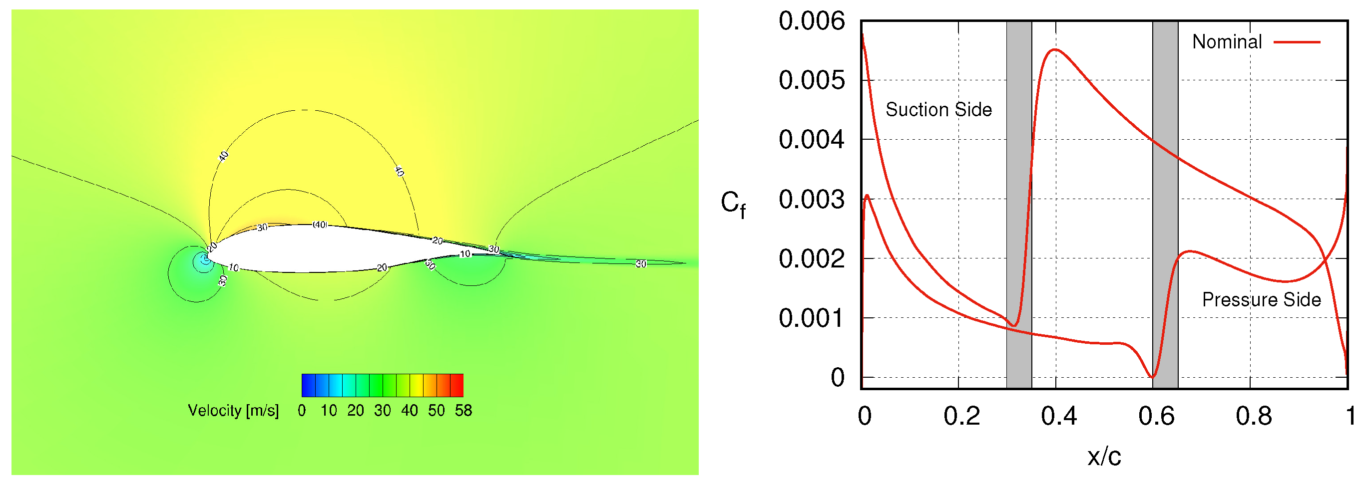
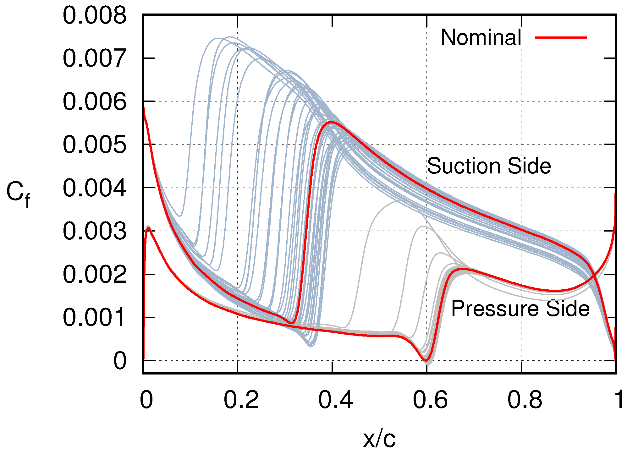
3.1. Case I—The NLF(1)-0416 Airfoil

The first case addresses the flow around a low-speed natural laminar flow (NLF) airfoil, namely the NLF(1)-0416 one [33]. The flow conditions are as follows: $M_{\infty }=0.1$, ${\alpha }_{\infty }=2.{03}^{\circ }$, $R{e}_c=4·{10}^6$ and the turbulence intensity is $Tu=0.15\%$. As this is a widely used test case for transition models [34], six structured meshes are publicly available: a tiny ($353\times 49$), a coarse ($529\times 73$), a medium ($705\times 97$), a fine ($1057\times 145$), an extra fine ($1409\times 193$) and an ultra fine ($2113\times 289$). On all these meshes, the prediction of the lift ($C_L$) and drag coefficient ($C_D$), for ${\alpha }_{\infty }=2.{03}^{\circ }$, shows that mesh independence is achieved for all meshes finer that the “Medium” one, as seen in

Table 1. Case I: Mesh independence study for the Spalart–Allmaras turbulence model coupled with the $\gamma -\tilde{R}{e}_{\theta t}$ transition model, at ${\alpha }_{\infty }=2.{03}^{\circ }$ and comparison with experimental data.

	Experimental	Tiny	Coarse	Medium	Fine	Extra	Ultra
$C_L$	0.672	0.7166	0.7075	0.7228	0.7230	0.7231	0.7235
$C_D$	0.0051	0.006673	0.007269	0.005984	0.005952	0.005930	0.005905

. Numerical results are also compared with the experimental data of [33], and a good agreement is obtained for both $C_L$ and $C_D$ values above the aforementioned mesh size. Therefore, in what follows, the “Medium” mesh is used.

A CFD analysis performed using the values of the transition model constants of Section 2.1 (to be referred to as the nominal ones), which compute the velocity magnitude isolines and the skin friction coefficient distribution along the airfoil contour shown in Figure 1. On the same plot, one may also see the experimentally measured [33] range of transition points; with the nominal constants, the CFD predicts them with acceptable accuracy. As a first conclusion, the computed $C_L$ and $C_D$ values as well the transition point location are in good agreement with the measurements, demonstrating the reliability of the CFD tool.

This case is used to quantify uncertainties in the $C_L$ and $C_D$ (two QoIs) caused by uncertainties in the values of the four ($M=4$) $\gamma -\tilde{R}{e}_{\theta t}$ model constants in Equations (5)–(8). Specifically, $c_{{\alpha }_1}$, $c_{{\alpha }_2}$, $c_{{ϵ}_2}$ and $c_{\theta ,t}$ are considered as uncertain variables with normal distribution as follows:

$$c_{{\alpha }_1}\sim \mathcal{N}(2.0,0.2),c_{{\alpha }_2}\sim \mathcal{N}(0.06,0.006),c_{{ϵ}_2}\sim \mathcal{N}(50.0,5.0),c_{\theta ,t}\sim \mathcal{N}(0.03,0.003)$$

(16)

The Latin hypercube sampling (LHS) method is used to generate 40 samples in the uncertain variables’ space. For the sampling, the bounds of each uncertain variable are defined as ±3 $\sigma$ with respect to their nominal (mean) value. This small number of samples was intentionally selected since 40 calls to the CFD tool correspond to half of the CFD runs (81 runs) needed to compute the statistical moments using the gPCE with the CFD tool (to be referred to as gPCE-CFD) and chaos order equal to 2 ($K=2$). Figure 2 illustrates the $C_f$ distributions for the 40 samples as well as the computation with the nominal values of the transition model constants. Changes in the model constants within the decided bounds significantly affect the transition point and, consequently, the QoIs. It seems that the uncertain space is adequately sampled.

Then, a single RBF network, with four inputs and two outputs, is trained and used for predicting the two QoIs. The computational cost to evaluate the RBF training patterns is forty time units, assuming that one time unit corresponds to the cost of running the CFD tool once. The RBF network training represents negligible cost. To assess the so-trained RBF network, 300 random samples (different than the 40 training patterns) are additionally generated; these are both evaluated on the CFD tool and approximated using the RBF-based surrogate. For these samples, the root mean square errors (RMSEs) for the two QoIs are ${\mathrm{RMSE}}_{C_L}=1.097·{10}^{-3}$ and ${\mathrm{RMSE}}_{C_D}=9.412·{10}^{-5}$. Both are considered to be absolutely satisfactory.

Given the above, the RBF network predictions can safely be used in UQ. In this case, comparison among all UQ methods of Section 2.5, using the RBF network, is carried out. In what follows, MC-RBF, gPCE-RBF and rPCE-RBF stand for a UQ using the MC, gPCE and rPCE methods, respectively, all of them based exclusively on the RBF model. For the MC, ${10}^4$ samples are generated at random. The gPCE used the 81 GQ points and the rPCE used either the 81 GQ points or the 150 samples generated using the LHS.

The obtained results are summarized in

Table 2. Case I: Statistical moments of the QoIs. Comparison of different UQ methods supported by the RBF or the CFD tool.

Method/Tool	Time Units	${\mathit{\mu }}_{{\mathit{C}}_{\mathit{L}}}$	${\mathit{\sigma }}_{{\mathit{C}}_{\mathit{L}}}$	${\mathit{\mu }}_{{\mathit{C}}_{\mathit{D}}}$	${\mathit{\sigma }}_{{\mathit{C}}_{\mathit{D}}}$
MC-RBF (${10}^4$)	40	0.7204	0.004567	0.006195	0.0004196
gPCE-RBF (81)	40	0.7204	0.004643	0.006194	0.0004266
rPCE-RBF (81)	40	0.7204	0.004548	0.006383	0.0004203
rPCE-RBF (150)	40	0.7204	0.004615	0.006446	0.0004148
gPCE-CFD (81)	81	0.7210	0.004923	0.006153	0.0004477
rPCE-CFD (81)	81	0.7207	0.004584	0.006386	0.0004198
rPCE-CFD (40)	40	0.7206	0.004547	0.006421	0.0004132

. The same table includes the outcomes of the gPCE-CFD and rPCE-CFD with 81 and 40 samples. The first column indicates the UQ method, the tool to compute or approximate the QoIs and (in parenthesis) the number of samples used. It can be seen that the statistical moments, especially those of $C_L$, are computed with high accuracy using the proposed RBF-based surrogate. Since, in this work, the interest is to assess the impact of the RBF models on UQ, whereas an MC-CFD run with ${10}^4$ replicates, which could give a dependable estimation of the statistical moments, should be avoided, a fair way to evaluate the results of Table 2 is to compare the results on a per-method basis. The comparison of gPCE-RBF with gPCE-CFD is excellent for the mean values and has some “expected” differences in the standard deviations. The rPCE-RBF and rPCE-CFD with 81 samples each are much closer, even in the prediction of the standard deviations. It can also be considered that the rPCE-CFD (81) is more accurate than rPCE-CFD (40), due to the double number of samples used. The MC-RBF performs an exhaustive sampling in the uncertain space and it seems that (based on additional tests not included in Table 2) no improvement is expected by further increasing the number of samples. Overall, one may notice the rather close results obtained by the MC-RBF and gPCE-RBF compared to those by the regression-based methods. The latter, either with the RBF or the CFD tool, over-predict the ${\mu }_{C_D}$ values. These differences also reflect the effect of the sampling method, i.e., the LHS in the cases with 40 and 150 samples instead of a sampling which considers the normal distributions of the uncertain variables. Thus, using MC-RBF or gPCE-RBF, reduction in the computational cost by $50\%$ is obtained, since the cost comes practically only from the 40 CFD evaluations of the training patterns, rather than the 81 CFD runs required for the gPCE-CFD.

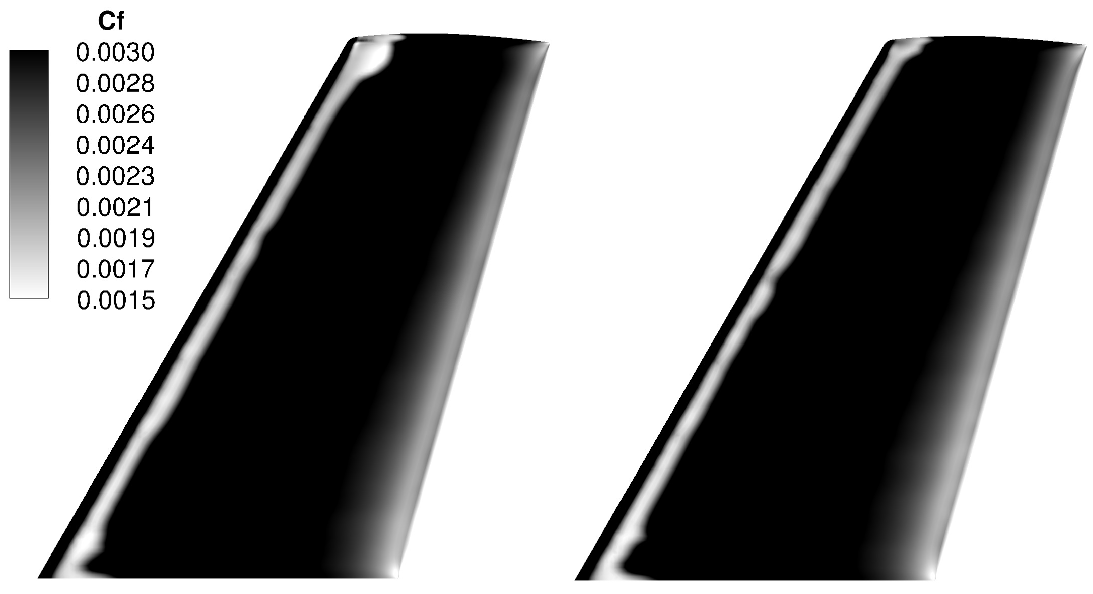
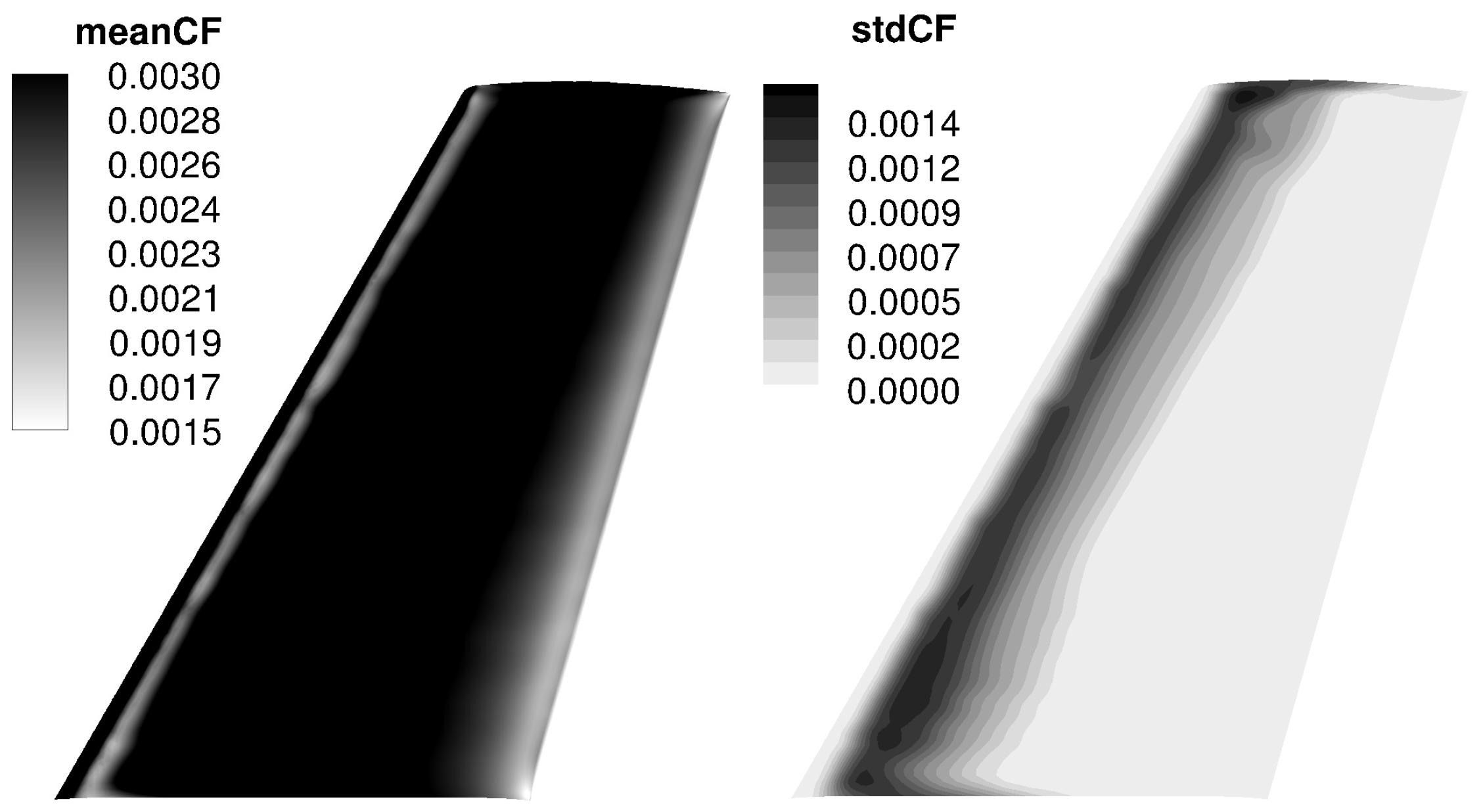
3.2. Case II—The ONERA M6 Wing

Case II addresses the flow around the ONERA M6 wing at $M_{\infty }=0.262$, $Re=3.5·{10}^6$, zero angle of attack and zero yaw angle, $Tu=0.2\%$ and surface roughness $h_{rms}=5$ $\mathsf{\mu }$m [35]. The $\gamma -\tilde{R}{e}_{\theta t}$ transition model with crossflow effects is used as the CFD tool. The skin friction coefficient ($C_f$) field on the wing surface computed using the nominal values of the transition model is presented in Figure 3. White areas indicate the first part of each side of the wing surface along which the flow remains laminar.

In this case, over and above the transition model constants, the surface roughness is the fifth uncertain variable with $h_{rms}\sim \mathcal{N}(5·{10}^{-6},1.6·{10}^{-6})$, so finally $M=5$. For the model constants, the distributions of Equation (16) are used. Initially, 80 samples in the uncertain variables’ space are generated using the LHS and used to train an RBF network to predict $C_D/C_L$. The so-trained RBF is then used for the three aforementioned UQ methods and the results are summarized in

Table 3. Case II: Statistical moments of the QoI ($C_D/C_L$). Comparison of different UQ methods supported by the RBF or the CFD tool.

Method/Tool	Time Units	${\mathit{\mu }}_{{\mathit{C}}_{\mathit{D}}/{\mathit{C}}_{\mathit{L}}}$	${\mathit{\sigma }}_{{\mathit{C}}_{\mathit{D}}/{\mathit{C}}_{\mathit{L}}}$
MC-RBF ($2·{10}^4$)	80	6.8200	0.3277
gPCE-RBF (243)	80	6.7946	0.3249
rPCE-RBF (243)	80	6.7975	0.3127
rPCE-RBF (120)	80	6.8442	0.3152
rPCE-RBF (80)	80	6.8603	0.3057
rPCE-CFD (120)	120	6.8571	0.3277
rPCE-CFD (80)	80	6.8635	0.3179

. For the MC method, $2·{10}^4$ replicates are selected, while for the gPCE-CFD the $3^5=243$ GQ points. For rPCE-RBF various numbers of samples are selected and tested, such as the 243 GQ points, the 80 initial samples or 120 samples. The use of gPCE-CFD is avoided due to its high computational cost as it requires 243 CFD runs for $K=2$. Instead, the rPCE-CFD with 80 and 120 samples is carried out. A good agreement in the statistical moments computed by implementing the RBF-based surrogate, with all the UQ methods, can be seen.

As in Case I, it is interesting to compare the rPCE-RBF (120) with rPCE-CFD (120) and the rPCE-RBF (80) with rPCE-CFD (80). The comparison is very satisfactory and the increase in the number of samples has the same effect. Surprisingly, the gPCE-RBF (243) and rPCE-RBF (243) compute a different mean value compared to all other methods and, also, differ from rPCE-RBF (120) which used half of the samples. For the MC-RBF, the comment is similar to the one made in Case I.

Figure 4 and Figure 5 present the statistical moments of $C_f$ computed using the gPCE-RBF method. The mean value plot on the surface shows a close similarity with the plot produced with the nominal values (Figure 3). Regarding the standard deviation of $C_f$, high values (dark area) appear close to the leading edge and this is a clear indication that these uncertainties affect a small area around the location of transition in Figure 3. In Figure 4 and Figure 5, one may see a narrow whitish zone, very close to the leading edge, which corresponds to the very first part of the wing where the flow is not affected in any case.

3.3. Case III—The S8052 Airfoil

The third case addresses the flow around the S8052 isolated airfoil. The flow conditions are as follows: $M_{\infty }=0.1$, ${\alpha }_{\infty }=3^o$, $R{e}_c=5.05·{10}^6$ and $Tu=1.28\%$ and the simulation uses the $\gamma -\tilde{R}{e}_{\theta t}$ transition model using the nominal values of the model constants, as seen in Section 2.1. Herein, two shape optimization problems, without and with geometric uncertainties, are considered. Geometric uncertainties are introduced using the KL expansion method. The RBF network is used as a surrogate to the CFD tool in order to approximate the QoI required for the computation of the statistical moments. The airfoil shape is parameterized using a $13 \times 9$ NURBS control lattice, as seen in Figure 6. Control points marked in red are allowed to be displaced in the normal-to-the chord direction, giving rise to $N=15$ design variables in total. For the case with geometric uncertainties, $M=18$ uncertain variables resulting from the KL expansion (see Equation (11)) are considered.

The LHS method is used to sample the design space, according to the ranges associated with the displaceable control points. A total of 200 different airfoil geometries are generated and evaluated on the CFD tool. The 198 y-coordinates of the nodal points along the contour of the airfoil are used as inputs to the RBF network. The selection of the nodal coordinates instead of those of the control points allows for the network to predict the $C_L$ and $C_D$ coefficients, not only in the case of a new airfoil geometry caused by changes in the design variables (in which case, the volumetric NURBS method undertakes the mesh displacement), but also when the shape is perturbed due to uncertainties. The computational cost for obtaining the training patterns is 200 time units. The cost for training the RBF network with 198 inputs and 2 outputs is rounded up to 1 time unit.

3.3.1. Shape Optimization without Uncertainties

The first shape optimization study is a shape optimization without uncertainties, for minimizing the drag-over-lift coefficient ratio, i.e., $F=C_D/C_L$. A comparison between the optimization run relying on the CFD tool and that on the RBF-based surrogate is made.

Once the RBF surrogate is available, at the cost of 201 time units, this is used as the sole evaluation tool during an EA-based search. The cost of an RBF-based evaluation is ∼1/30 time units (this is, in fact, the cost for creating the airfoil contour using the parameterization model) and a limit of 300 evaluations on the RBF model is set. Upon termination of the EA run, the 10 best individuals seen during the search, excluding some of the top solutions that are close enough (in the design space) to an even better solution, are selected for possible re-evaluation on the CFD tool. The final number of individuals to be re-evaluated on the CFD tool is determined by the RBF prediction accuracy, the percentage error of which should not exceed $1\%$. Herein, after the first 300 evaluations on the RBF model, 10 shapes solutions are re-evaluated (at the cost of 10 time units), since the mean percentage error of $C_D$ predictions is $1.7\%$, whereas that of $C_L$ is $0.07\%$. The successive steps that are formed by the RBF network training, the EA-based search on it and the best solutions re-evaluations on the CFD tool constitute an optimization cycle. Therefore, once the 10 re-evaluated individuals are appended to the training patterns, a new RBF network is trained and a second optimization cycle starts. In the second cycle, five re-evaluations are sufficient to lower the mean percentage error of $C_D$ at $0.8\%$. The convergence history of this procedure is presented in Figure 7. The optimization terminates after three cycles, since the RBF predictions reach the required level of accuracy and a noticeable improvement in the objective function is no longer expected.

To quantify the gain from the use of the RBF-based surrogate, the optimization problem is additionally solved using an EA relying exclusively on the CFD tool. Since we are dealing with a stochastic optimization method, three runs are performed using different random number generator seeds. A termination criterion of 500 CFD evaluations (500 time units) is set and the corresponding convergence histories as well as the average of the three runs are shown in Figure 8. The best solutions of the three cycles of the run on the RBF-based surrogate, after being re-evaluated on the CFD tool, are also included. It can be seen that, with the RBF-based surrogate, one may obtain a solution of, practically, the same quality (almost the same objective function value) at a significantly lower computational cost.

3.3.2. Shape Optimization under Geometric Uncertainties

Here, uncertainties in the airfoil geometry are additionally introduced. The latter are modeled with the KL expansion presented in Section 2.2, using $M=18$ uncertain variables. The $C_D/C_L$ is selected as the QoI (J) and the objective function to be minimized during the shape optimization is the sum of the mean value and standard deviation of J, namely $F={\mu }_J+{\sigma }_J$, corresponding to a possible worst-case scenario. For the computation of ${\mu }_J$ and ${\sigma }_J$, both the MC-RBF and rPCE-RBF are used. To do so, for each new nominal airfoil resulting from a change in the design variables, 1000 imperfect (perturbed) geometries are generated using the KL expansion. The selected number of perturbed geometries is adequate for the rPCE that needs to compute 190 coefficients (for chaos order 2) and a compromise for the MC that, otherwise, would ask for thousands of perturbed geometries. In this case, each evaluation (UQ) takes $0.15$ time units and a termination criterion of 200 time units, over and above those required for the RBF training (200 time units), is set. The convergence histories of these optimization runs are shown in Figure 9.

The optimized shapes from both methods are re-evaluated on the CFD tool; this is a very costly task as it requires 1000 CFD simulations, one for each imperfect geometry resulting from the KL expansion. For these simulations, the RBF-based mesh displacement tool of Section 2.2 is used to avoid re-meshing each imperfect geometry. A comparison of the F and the statistical moments of the QoI with those of the baseline geometry is given in

Table 4. Case III: Comparison of the objective function F and statistical moments of J of the baseline and the optimized solutions (re)-evaluated on the CFD tool.

Geometry/Method	F	${\mathit{\mu }}_{\mathit{J}}$	${\mathit{\sigma }}_{\mathit{J}}$
Baseline	0.0172588	0.01694	0.0003188
Optimized (using MC-RBF)	0.0134667	0.01317	0.0002967
Optimized (using rPCE-RBF)	0.0134317	0.01314	0.0002917

. In either case, the optimized geometry is better than the baseline one. The use of the RBF-based surrogate makes such an optimization run feasible, since running 1000 CFD simulations for each candidate solution noticeably increases the computational cost.

4. Discussion—Conclusions

The purpose of this paper was to assess different ways of using radial basis function (RBF)-based surrogate models in UQ and CFD shape optimization with uncertainties. Initially, an RBF surrogate that predicts the QoI supports the Monte Carlo, GQ and regression PCE methods which perform the UQ. Uncertainties were firstly related to a widely used transition model with coefficients tuned according to experimental data and that, as such, carry uncertainties. Two UQ studies, for an NLF airfoil and a wing, showed that the RBF model may effectively support the above UQ methods and reduce the overall computational cost by even $50\%$, compared to the same method that uses the CFD tool. The error, due to the use of the RBF model, in the first statistical moments of the lift and drag coefficients was very low and this made it a dependable UQ model for use in optimization loops. For the sake of pluralism, to assess the use of the RBF-based UQ in optimization under uncertainties, a shape optimization problem with geometrical uncertainties was selected. Perturbed shapes are obtained through the Karhunen–Loève technique. The optimization was based on an evolutionary algorithm. Since for each candidate solution (new geometry) hundreds of perturbed geometries must be evaluated, all these computations of the QoI were performed at low cost using the RBF surrogate model, instead of the CFD tool. The latter is by orders of magnitude more expensive than the former, offering a huge saving in computational cost.

References

1. Xiu, D.; Karniadakis, G. Modeling uncertainty in flow simulations via generalized polynomial chaos. J. Comput. Phys. 2003, 187, 137–167. [Google Scholar]
2. Najm, H.N. Uncertainty quantification and polynomial chaos techniques in Computational Fluid Dynamics. Annu. Rev. Fluid Mech. 2009, 41, 35–52. [Google Scholar]
3. Dinescu, C.; Smirnov, S.; Hirsch, C.; Lacor, C. Assessment of intrusive and non-intrusive non-deterministic CFD methodologies based on polynomial chaos expansions. Int. J. Eng. Syst. Model. Simul. 2010, 2, 87–98. [Google Scholar]
4. Schillings, C.; Schmidt, S.; Schulz, V. Efficient shape optimization for certain and uncertain aerodynamic design. Comput. Fluids 2011, 46, 78–87. [Google Scholar]
5. Chatzimanolakis, M.; Kantarakias, K.D.; Asouti, V.; Giannakoglou, K. A painless intrusive polynomial chaos method with RANS-based applications. Comput. Methods Appl. Mech. Eng. 2019, 348, 207–221. [Google Scholar]
6. Eldred, M.S.; Burkardt, J. Comparison of non-intrusive polynomial chaos and stochastic collocation methods for uncertainty quantification. In Proceedings of the 47th AIAA Aerospace Sciences Meeting including The New Horizons Forum and Aerospace Exposition, Orlando, FL, USA, 5–8 January 2009. [Google Scholar]
7. Hosder, S.; Walters, R.W. Non-intrusive polynomial chaos methods for uncertainty quantification in fluid dynamics. In Proceedings of the 48th AIAA Aerospace Sciences Meeting including the New Horizons Forum and Aerospace Exposition, Orlando, FL, USA, 4–7 January 2010. [Google Scholar]
8. Walters, R.W.; Huyse, L. Uncertainty analysis for fluid mechanics with applications. In NASA Technical Report 2002-1; NASA: Washington, DC, USA, 2002. [Google Scholar]
9. Haldar, A.; Mahadevan, S. Probability, Reliability and Statistical Methods in Engineering Design; John Wiley & Sons: New York, NY, USA, 2000. [Google Scholar]
10. Putko, M.; Taylor, A.; Newman, P.; Green, L. Approach for input uncertainty propagation and robust design in CFD using sensitivity derivatives. J. Fluids Eng. 2002, 124, 60–69. [Google Scholar]
11. Skamagkis, T.; Papoutsis-Kiachagias, E.; Giannakoglou, K. CFD-based shape optimization under uncertainties using the Adjoint-assisted polynomial chaos expansion and projected derivatives. Comput. Fluids 2022, 241, 105458. [Google Scholar]
12. Liu, Y.; Wang, D.; Sun, X.; Liu, Y.; Dinh, N.; Hu, R. Uncertainty quantification for multiphase-CFD simulations of bubbly flows: A machine learning-based Bayesian approach supported by high-resolution experiments. Reliab. Eng. Syst. Saf. 2021, 212, 107636. [Google Scholar]
13. Evangelista, F., Jr.; Almeida, I.F. Machine learning RBF-based surrogate models for uncertainty quantification of age and time-dependent fracture mechanics. Eng. Fract. Mech. 2021, 258, 108037. [Google Scholar]
14. Ansari, A.; Mohaghegh, S.D.; Shahnam, M.; Dietiker, J.F. Modeling average pressure and volume fraction of a fluidized bed using data-driven smart proxy. Fluids 2019, 4, 123. [Google Scholar]
15. Duraisamy, K.; Zhang, Z.J.; Singh, A.P. New approaches in turbulence and transition modeling using data-driven techniques. In Proceedings of the 53rd AIAA Aerospace Sciences Meeting, Kissimmee, FL, USA, 5–9 January 2015. [Google Scholar]
16. Song, Z.; Liu, Z.; Lu, J.; Yan, C. Quantification of parametric uncertainty in γReθ model for typical flat plate and airfoil transitional flows. Chin. J. Aeronaut. 2023, 36, 237–251. [Google Scholar] [CrossRef]
17. Jakobsson, S.; Amoignon, O. Mesh deformation using radial basis functions for gradient-based aerodynamic shape optimization. Comput. Fluids 2007, 36, 1119–1136. [Google Scholar] [CrossRef]
18. Biancolini, M.; Viola, I.; Riotte, M. Sails trim optimisation using CFD and RBF mesh morphing. Comput. Fluids 2014, 93, 46–60. [Google Scholar] [CrossRef]
19. Gagliardi, F.; Giannakoglou, K. A two-step Radial Basis Function-based CFD mesh displacement tool. Adv. Eng. Softw. 2019, 128, 86–97. [Google Scholar] [CrossRef]
20. Kampolis, I.; Trompoukis, X.; Asouti, V.; Giannakoglou, K. CFD-based analysis and two-level aerodynamic optimization on Graphics Processing Units. Comput. Methods Appl. Mech. Eng. 2010, 199, 712–722. [Google Scholar] [CrossRef]
21. Spalart, P.; Allmaras, S. A one-equation turbulence model for aerodynamic flows. Rech. Aerosp. 1994, 1, 5–21. [Google Scholar]
22. Piotrowski, M.; Zingg, D. Smooth local correlation-based transition model for the Spalart-Allmaras turbulence model. AIAA J. 2020, 59, 474–492. [Google Scholar] [CrossRef]
23. Trompoukis, X.; Tsiakas, K.; Asouti, V.; Giannakoglou, K. Continuous adjoint-based optimization of a turbomachinery stage using a 3D volumetric parameterization. Int. J. Numer. Methods Fluids 2023, 6, 20. [Google Scholar] [CrossRef]
24. Piegl, L.; Tiller, W. The NURBS Book; Springer: Berlin/Heidelberg, Germany, 1995. [Google Scholar]
25. Fong, W.; Darve, E. The black-box fast multipole method. J. Comput. Phys. 2009, 228, 8712–8725. [Google Scholar] [CrossRef]
26. Karimi, M.S.; Raisee, M.; Farhat, M.; Hendrick, P.; Nourbakhsh, A. On the numerical simulation of a confined cavitating tip leakage vortex under geometrical and operational uncertainties. Comput. Fluids 2021, 220, 104881. [Google Scholar] [CrossRef]
27. Ghanem, R.; Spanos, P. Stochastic Finite Elements: A Spectral Approach; Springer: New York, NY, USA, 1991. [Google Scholar]
28. Le Maitre, O.P.; Knio, O.M. Spectral Methods for Uncertainty Quantification with Applications to Computational Fluid Dynamics; Springer: Berlin/Heidelberg, Germany, 2010; Volume 718. [Google Scholar]
29. Cho, H.; Venturi, D.; Karniadakis, G. Karhunen–Loève expansion for multi-correlated stochastic processes. Probabilistic Eng. Mech. 2013, 34, 157–167. [Google Scholar] [CrossRef]
30. Haykin, S.S. Neural Networks and Learning Machines, 3rd ed.; Pearson Education: London, UK, 2009. [Google Scholar]
31. Xiu, D.; Hesthaven, J. High-Order collocation methods for differential equations with random inputs. SIAM J. Sci. Comput. 2005, 27, 1118–1139. [Google Scholar] [CrossRef]
32. Zhao, H.; Gao, Z.; Gao, Y.; Wang, C. Effective robust design of high lift NLF airfoil under multi-parameter uncertainty. Aerosp. Sci. Technol. 2017, 68, 530–542. [Google Scholar] [CrossRef]
33. Somers, D.M. Design and experimental results for a Natural-Laminar-Flow airfoil for general aviation applications. In NASA Technical Paper 1861; NASA: Washington, DC, USA, 1981. [Google Scholar]
34. Coder, J.G. Standard test cases for CFD-based laminar-transition model verification and validation. In Proceedings of the 2018 AIAA Aerospace Sciences Meeting, Kissimmee, FL, USA, 8–12 January 2018. [Google Scholar]
35. Schmitt, V.; Cousteix, J. Etude de la Couche Limite Tridimensionnelle sur une Aile en Fleche; Technical Report No 14/1713 AN; ONERA: Meudon, France, 1975. [Google Scholar]
Figure 1. Case I: (Left) Velocity magnitude field around the airfoil computed using the nominal values of all model constants. (Right) Skin friction coefficient ( C f ) distribution along the airfoil contour as computed using the CFD tool. The vertical zones in grey represent ranges of the measured [33] transition points on both airfoil sides.
Fluids 08 00292 g001
Figure 2. Case I: Skin friction coefficient ( C f ) distributions along the pressure (grey curves) and suction (greyish-blue curves) sides of the 40 training patterns. Curves computed using the nominal values of the γ R ˜ e θ t model constants are included in red, too.
Fluids 08 00292 g002
Figure 3. Case II: Skin friction coefficient ( C f ) over the wing surface, as computed by the CFD tool. (Left) Suction side. (Right) Pressure side.
Fluids 08 00292 g003
Figure 4. Case II: Statistical moments of C f over the suction side. (Left) Mean value. (Right) Standard deviation.
Fluids 08 00292 g004
Figure 5. Case II: Statistical moments of C f over the pressure side. (Left) Mean value. (Right) Standard deviation.
Fluids 08 00292 g005
Figure 6. Case III: NURBS control lattice used for the parameterization. Control points in black remain fixed, while the red ones are allowed to be displaced in the normal-to-the chord direction.
Fluids 08 00292 g006
Figure 7. Case III: Convergence history of the shape optimization run relying on the RBF-based surrogate (purple line with empty circles) with re-evaluation on the CFD tool (filled red circles). The vertical axis values indicate either the RBF-based predictions (for the EA convergence histories; purple lines) or the objective function values computed by the CFD tool for the re-evaluated solutions. The horizontal axis starts after the first 201 time units to include the cost for evaluating the training patterns (200 CFD runs, i.e., 200 time units) and training the RBF (1 time unit).
Fluids 08 00292 g007
Figure 8. Case III: Convergence histories of the optimization runs relying on the CFD tool with different initializations of the EA (three blue lines) and their averaged (black). The filled red circles indicate the re-evaluated (on the CFD) outcomes of the three cycles of the EA optimization on the RBF.
Fluids 08 00292 g008
Figure 9. Case III: Convergence histories of the optimization runs under geometric uncertainties. The vertical axis corresponds to values of F predicted by the RBF model.
Fluids 08 00292 g009