Article

Numerical Study of a Small Horizontal-Axis Wind Turbine Aerodynamics Operating at Low Wind Speed

by
Somaya Younoussi
* and
Abdeslem Ettaouil
Mechanical Engineering Department, Mohammadia School of Engineers, Mohammed V University, Rabat 10090, Morocco
*
Author to whom correspondence should be addressed.
Fluids 2023, 8(7), 192; https://doi.org/10.3390/fluids8070192
Submission received: 19 May 2023 / Revised: 5 June 2023 / Accepted: 20 June 2023 / Published: 26 June 2023
(This article belongs to the Section Mathematical and Computational Fluid Mechanics)

Abstract

:
The present work aims to study the aerodynamic characteristics of a newly designed three-bladed horizontal-axis wind turbine (HAWT) using the Computational Fluid Dynamic (CFD) method. The blade geometry is designed using an improved Blade Element Momentum (BEM) method to be similar in size to the Ampair300 wind turbine. The shear stress transport (SST) transition turbulence model closure is utilized to solve the steady state three-dimensional Reynolds Averaged Navier-Stokes (RANS) equations. The Ansys Fluent CFD solver is used to solve the problem. Then, a comparison between the two turbines’ operating conditions is conducted by monitoring the pressure coefficient, pressure contours and velocity vectors at five different radial positions. The analysis of the Tip Speed Ratio (TSR) effects on the turbine efficiency and on the flow behavior on the blade and in the near wake is carried out. For 8 m/s wind speed, the optimum pitch angle is also investigated, and the results are prepared against each TSR.

1. Introduction

In recent years, the expanding population and strong economic growth, along with the accompanying living standard changes, has increased the demand for energy. The worldwide consumption of petroleum and other liquid fuels increased from 90 million barrels per day in 2012 to 98.3 million b/d in March 2022 [1], and is expected to reach 121 million b/d in 2040 [2]. The extensive consumption of fossil fuels, the primary source of CO2 emissions, threatens human health, quality of life, ecological balance and biological diversity [3]. Therefore, in order to deplete the use of fossil fuels and, at the same time, satisfy the rising demand for energy, the use of clean and renewable energy sources is becoming a necessity rather than a choice. Among all of the renewable energies, wind energy is ideally placed to confront this energy transition because of its rapid emerging technology, efficiency gains and cost competitiveness [3,4]. The worldwide cumulative onshore and offshore wind power installations capacity rose from 7.5 GW in 1997 [5] to up to 837 GW by the end of 2021, which has reduced CO2 emissions by 1.2 billion tons globally [6].
The Blade Element Momentum (BEM) and Computational Fluid Dynamics (CFD) theories are the most commonly used methods for predicting the aerodynamic performance of wind turbines and providing their aerodynamic characteristics. The application of CFD methods in engineering problems dates back to the mid-1960s, where the Imperial College (IC) group, led by Prof. Spalding [7], revolutionized the analysis of fluids in motion through computer modelling by developing viable numerical discretization methods, robust flow solvers and practical models for turbulence. Since then, CFD has become a valuable asset for engineers and researchers in a wide range of applications. In 2013, the CFD business reached a value of USD 1.0 billion, with a growth rate of around 10% in industry and academia, with North America and Asia as major users [8]. In the past two decades, thanks to the vast advances in hardware computing and numerical software modelling capabilities, rigorous simulations and optimization techniques applied to large scale problems are already feasible [8]. As a result, RANS-based models are now able to be applied to more complex flow problems, and the use of LES-based models are now possible [9]. Hence, the development in CFD modelling has covered advanced atmospheric boundary layer simulation in complex terrains such as cliffs or wake-wake interaction [9].
Its simpler codes and low computation cost make the BEM method highly preferred by several wind turbine industries in both design and performance analysis. Gupta et al. [10] designed two different rotors using the BEM theory. Initially, a selection of airfoils that provide the maximum lift to drag ratio was conducted. The rotor 1 was designed using SG6050 and SG6043 airfoils, while the rotor 2 was designed using E555 and E216 airfoils. According to the BEM theory, rotor 1 presented a better performance than rotor 2 in terms of the power coefficient, recording a Cp of 0.445 for a tip speed ratio of 7 and at a wind speed of 6 m/s. Then, CFD analysis of this rotor was investigated at these conditions, and the obtained power coefficient was 0.35687. Another new mixed airfoil wind turbine was designed by Hassan et al. [11] using S1210 and S1223 airfoils. The chord and twist angles were determined using the optimal angle of attack, extracted through the Xfoil tool at the designed wind speed. The BEM theory and Q’blade software were used to maximize the power coefficient at low wind speeds. At a wind speed of 7 m/s, the power coefficient of the new blade design was 0.47, whereas it was found to be equal to 0.43 when the CFD analysis of this blade was carried out. In their work, Muhsen at al. [12] developed a wind blade design approach that allows to optimize the design parameters, in addition to the blade geometry. The airfoils that provide the best pitch angles for the design wind speed were firstly selected using Xfoil tool. A MATLAB program was then used to determine the optimal design parameters and to find thereafter the optimal chord and AoA enabled a maximum power coefficient to be recorded at each blade section for these optimal parameters. The obtained blade design was analyzed and further improved using the Q’blade software. The BEM theory was utilized to optimize the tip speed ratio in order to find the maximum possible power coefficient with this blade. The resulting blade design recorded a power coefficient of 0.445 with an optimal tip speed ratio of 6.5 at a wind speed of 5.5 m/s. For more practical wind blade design in manufacturing, Yang [13] designed a wind blade using the linearization method of chord and twist distributions. This method was implemented to improve the 5-MW NREL wind turbine. Initially, the ideal blade geometry was determined using the BEM theory. Then, a linearization method was applied to the chord and the twist distributions. A performance analysis was conducted by testing different coefficients of the linear functions at each TSR value in order to improve the power coefficient. The results showed that the new design improved the NREL 5 MW performance at low wind speeds.
As a result of the simultaneous presence of three-dimensionality, unsteadiness and the rotational and turbulence effects, the BEM theory failed in many cases to predict the HAWT performances. In these cases, the CFD technique, as a more sophisticated and cost-effective tool, is widely used. As there is no unique or recommended CFD model for wind turbine aerodynamic simulations, many studies on CFD are found in the literature. For example, Plaza et al. [14] conducted an aerodynamic analysis of a wind turbine rotor using the two above-mentioned methods. The forces, pressure and torque generated in the rotor are computed using BEM and CFD and are compared to the experimental data. At low and medium velocity, the BEM theory provided better results than the RANS-CFD method. However, when the wind velocity was high enough to produce flow separation, the BEM failed, whereas the RANS-CFD simulations showed good agreement with the experimental data over the whole range of wind velocity. Bangga [15] analyzed the aerodynamic performance of a large 10 MW HAWT using the BEM and CFD methods. Their finding revealed that to ensure the accuracy of the BEM theory, it is important to use a hybrid polar dataset for BEM calculations. Along the blade, with the exception of the tip region, 3D polar data were recommended, which were obtained from the 3D CFD simulations. However, in the tip region, the 3D polar was unable to use the tip loss correction in the BEM calculation; as a result, the 2D polar data were used. Hence, by using this hybrid polar in the calculation, the comparison between BEM and CFD shows an excellent agreement for all blade sections, even at a high wind speed, where massive flow separation takes place in the inboard area. Keerthana et al. [16] designed a scaled model of a 3 kW horizontal axis wind turbine using the BEM theory and then studied the variation of the torque, normal force and power with the wind speed using Gambit as a pre-processor and Fluent as a post-processor. A steady RANS-k-ω-SST method was used. The results showed good agreement with theoretical trend. Khlaifat et al. [17] investigated the effect of four RANS turbulence models in predicting the aerodynamics of a 20 kW horizontal axis wind turbine. At low wind speeds where the flow is attached, all four RANS models presented good agreement with the measured data. However, at 9 m/s where the stall onset occurs due to laminar-to-turbulent transition phenomenon, the transition SST model made the best prediction accuracy. At high wind speeds exceeding 10 m/s, all tested RANS models were unable to predict the turbine’s aerodynamics due to the separation of the flow and the stall phenomena.
In the present work, an aerodynamic study of a newly designed three-bladed horizontal axis wind turbine is investigated using the CFD technique. The design of the blade is created via an improved BEM method to be similar in size to the Ampair300 turbine, which is used to validate the CFD results. Then, a steady state simulation of the resulting blade is investigated using three turbulence models: Spalart-Allmaras, k-ω SST and SST transition. The best performing CFD model will be used thereafter to study the aerodynamic characteristics of the rotor. The pressure coefficient distribution, the pressure contours and the velocity vectors of the blade at two operating conditions—8 m/s-52.659 rad/s and 12.6 m/s-111,701 rad/s—are obtained, analyzed and compared. The flow behavior around the blade is determined, involving the laminar-turbulent transition and separation phenomena in these two pre-mentioned cases. The effects of the Tip Speed Ratio (TSR) on the blade efficiency and the flow behavior on the blade and in the near wake are evaluated at a fixed wind speed of 8 m/s. Finally, the pitch angle effects on the turbine’s efficiency are investigated for the same fixed wind speed of 8 m/s.

2. Mathematical Model

2.1. Wind Turbine Geometry

In order to enhance the efficiency of the wind turbine at low wind speeds, a new blade was designed to be similar in size to the Ampair300 wind turbine [18]. An improved BEM method developed in a previous work [19] was applied to the NACA4418 wind turbine. The design approach consisted of maximizing the power coefficients at each blade section by calculating the axial induction factor using an iterative method. By introducing Equation (1) of tangential induction factor a’, the optimal chord and twist angle distributions were calculated using Equations (2) and (3), respectively.
a = 0.5 [ ( 1.0 + m λ r ) + ( 1 + m λ r ) 2 4 λ r 2 [ a 2 a ( 1 m λ r ) ] ]
where m = C D C L .
c = 8 π r a F ( 1 a F ) ( sin φ ) 2 B C n ( 1 a ) 2
θ = φ α o p t
where:
CD: Airfoil drag coefficient.
CL: Airfoil lift coefficient.
λr: Local tip speed ratio.
F: Glauert tip loss correction factor which is expressed as:
F = 2 π arccos ( e B ( R r ) 2 r 1 + a 1 a λ r )
φ: The relative inflow angle.
αopt: The optimal angle of attack.
R: Blade radius.
r: Hub radius.
B: The number of blades (B = 3).
Cn: The normal load coefficient is defined as:
a F ( 1 a F ) ( 1 a ) 2 = σ C n 4 ( sin φ ) 2
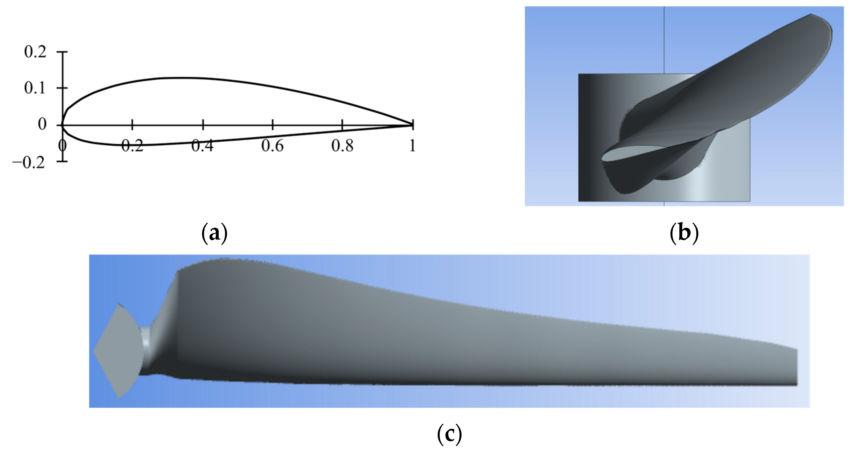
The tip speed ratio was then varied in order to improve the power coefficient. The maximum power coefficient of 0.463 was obtained at λ = 5. The main characteristics of the designed wind turbine blade are summarized in Table 1. Figure 1 shows the distribution of the chord and the twist angle along the blade. The blade shape is illustrated in Figure 2.

2.2. Mesh Generation

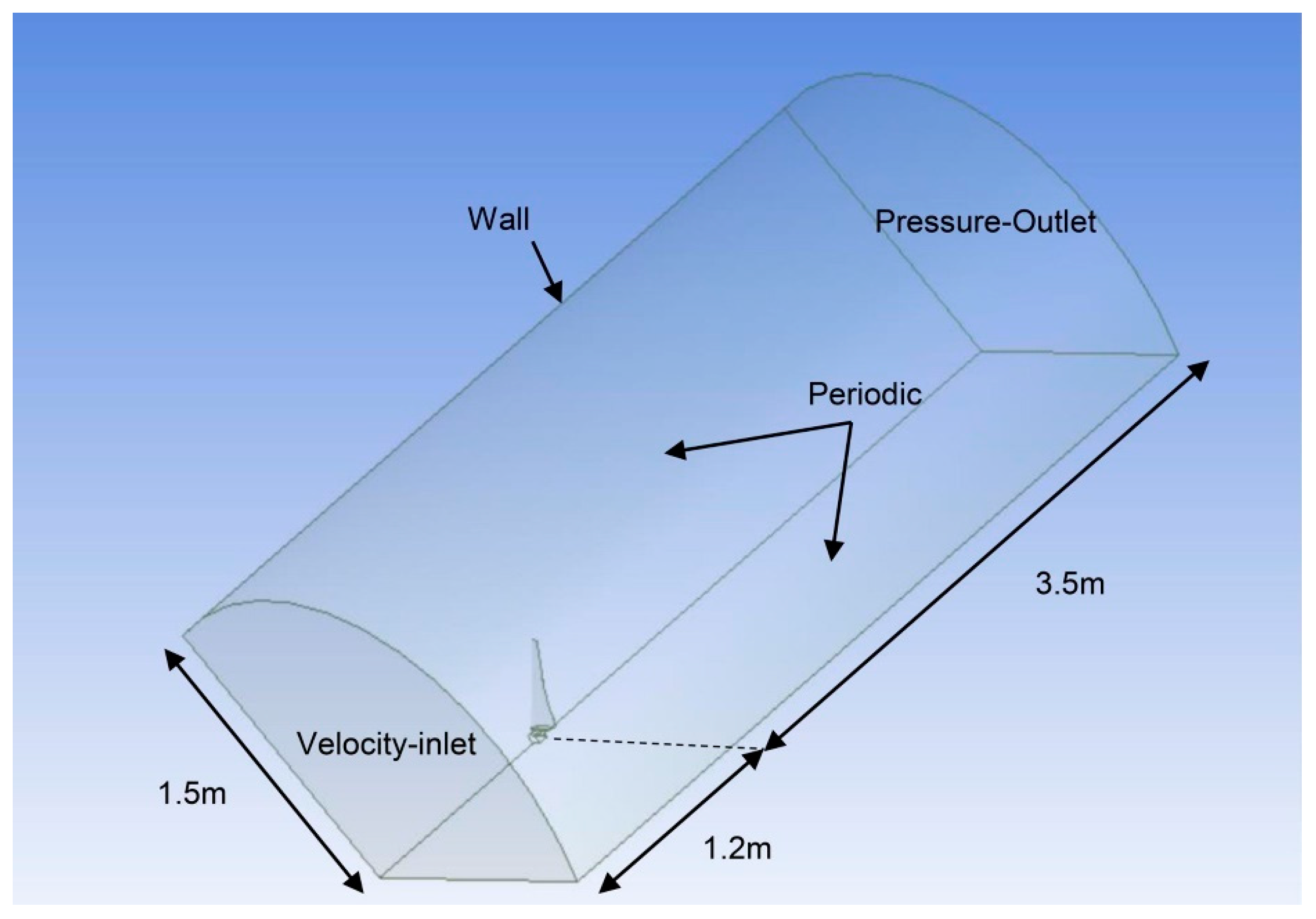
Due to the periodicity of the problem, the designed blade with a pitch angle of 10° is placed in a fluid domain, as shown in Figure 3, which consists of a 1/3 cylinder with a radius of 1.5 m and a length of 4.7 m. The upstream inlet boundary is defined at 1.2 m in front of the blade, whereas the downstream outlet boundary is specified to 3.5 m behind the blade.
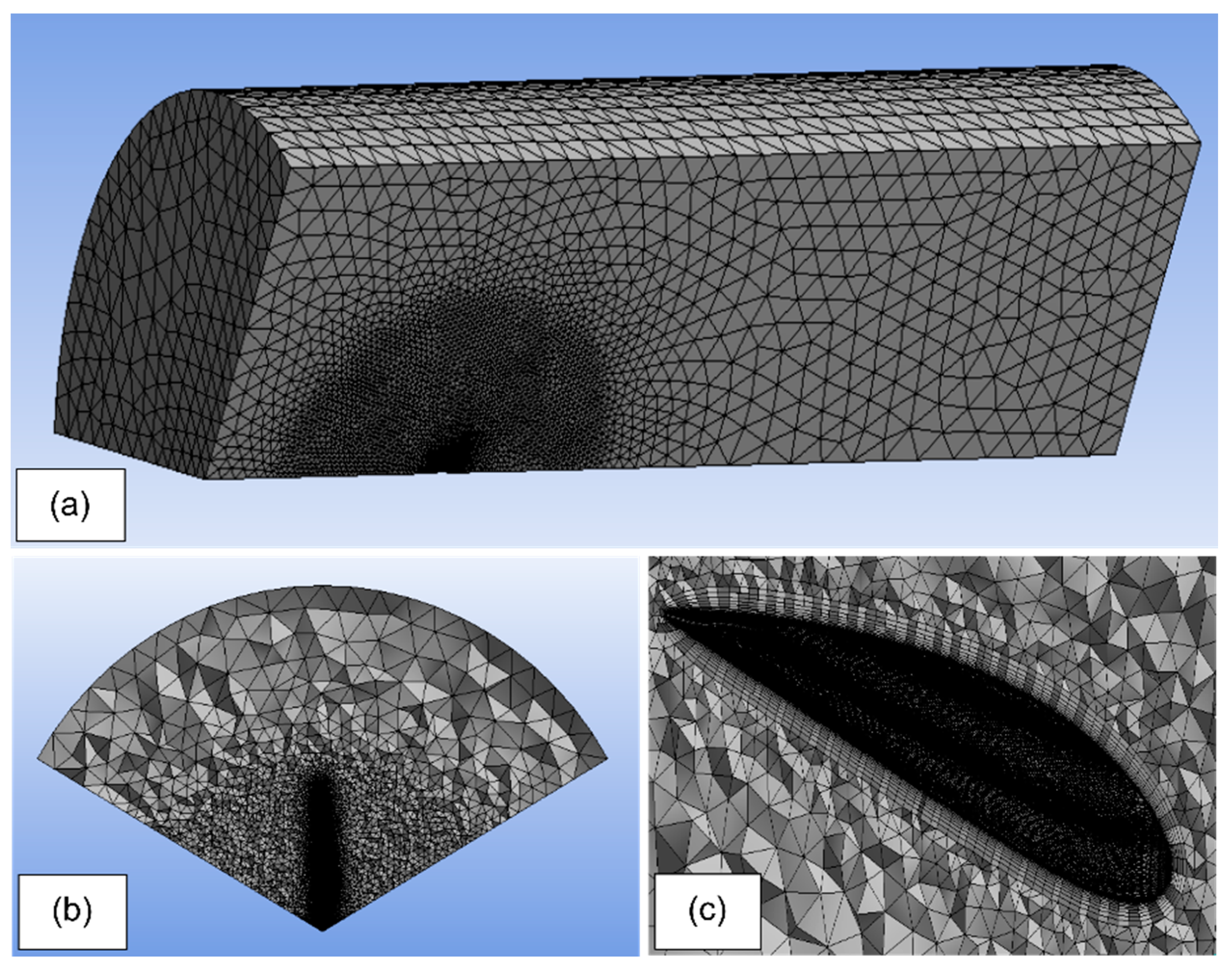
The Ansys meshing is used to generate a hybrid mesh comprising of structured prismatic mesh around the blade surface and unstructured tetrahedral mesh in the rest of the fluid domain. The proximity and curvature sizing functions are specified at the global level. The maximum face and tetrahedron sizes are 300 mm and 600 mm, respectively. A finer mesh is created around the rotor using a sphere influence of a 700 mm radius with a mesh size of 30 mm. The element size of the rest of the domain is 200 mm. The turbulence model used in the present study necessitates a value of wall y+ of approximately 1 to arrest the boundary layer behavior [20]. Therefore, 20 inflation layers with a first layer thickness of 0.00825 mm and growth rate of 1.25 are inserted around the blade surface, as shown in Figure 4c. Prior to the study, it was crucial to conduct a mesh independence study by testing seven different mesh sizes on the blade surface, as shown in Table 2, by monitoring the mechanical torque. The generated mesh is shown in Figure 4.

2.3. Computational Analysis

The CFD modelling of the horizontal axis wind turbine is carried out using a numerical resolution of the Reynolds Average Navier Stocks equations. The Ansys Fluent CFD solver based on the finite-volume method is used to solve the problem. In order to close the system, these equations are combined with a turbulence model.
The single reference frame (SRF) [21] is used to simulate rotor rotation. In this approach, the rotor is kept at rest, whereas the surrounding fluid domain is put into motion. Similarly, a steady simulation of the flow around the rotor is possible.
The expression of the fluid velocities in the rotating frame is conducted using the right hand thumb rule and is given by Equation (1):
V r = V a + Ω r ,
The governing average Navier-Stocks equations can be written in the framework of SRF, as follows:
V r ¯ = 0 ,
( V r ¯ V r ¯ ) + 2 ( Ω ¯ V r ¯ ) + [ Ω ¯ ( Ω ¯ r ¯ ) ] = ρ f ¯ p ¯ + ( μ + μ t ) · ( V r ¯ ) ,
where 2 ( Ω ¯ V r ¯ ) + [ Ω ¯ ( Ω ¯ r ¯ ) ] presents the Coriolis and centrifugal accelerations, f is the gravity vector, p is the pressure; μ and μt are, respectively, the kinematic and the turbulent kinematic viscosity of the fluid.
The choice of the appropriate fluid turbulence model is a major challenge in the CFD modelling of a wind turbine. In this work, the Spalart-Allmaras (SA) [22] turbulence model is used in the grid convergence study because of its low calculation time. Then, a comparison between the wind turbine generated power using SA, k-ω SST [23] and the transition SST [24] turbulence models is made. The transition SST is based on SST k-ω transport equations coupled with two additional transport equations, one for the intermittency (γ) and the other for the transition onset criteria in terms of the momentum-thickness Reynolds number (Reθ):
( ρ γ ) t + ( ρ U j γ ) x j = P γ 1 E γ 1 + P γ 2 E γ 2 + x j [ ( μ + μ t σ γ ) γ x j ] ,
( ρ Re θ t ˜ ) t + ( ρ U j Re θ t ˜ ) x j = P θ t + x j [ σ θ t ( μ + μ t ) Re θ t ˜ x j ]

2.4. Numerical Solution

In this simulation, the flow is imposed in the (0,0,1) direction. For validation and mesh sensitivity study purposes, the inlet velocity is specified as 8 m/s. In the outlet boundary layer, zero-gauge static pressure is applied. The reference frame attached to the fluid domain is set to rotate at an angular velocity of −52.659 rad/s. The blade surface is defined as a no-slip wall rotating with a zero angular velocity according to the adjacent cells.
The steady-state, pressure-based method combined with an absolute velocity formulation is used to solve the incompressible RANS models. A semi-implicit method,—SIMPLE [25]—is used to model the velocity and pressure in the momentum and the continuity equations.
The second-order upwind scheme is used for solving all transport and momentum equations of the simulations. The least squares cell-based method is applied for the spatial discretization gradient scheme. A standard discretization scheme is employed in the pressure values interpolation.
The residual values method is the most commonly used method for evaluating the convergence of the CFD solution. In this study, the residual values of six variables are monitored during the calculation process. The solution is considered to be converged when most of the residuals reach 10−5.
Due to the non-linear nature of the fluid flow, the solution should be calculated iteratively. A standard initialization method is applied, where the inlet boundary layer is used for calculating the initial values. After the solution’s convergence, the output results in terms of the aerodynamic power are validated against the experimental data.

3. Results and Discussion

3.1. Grid Convergence Study

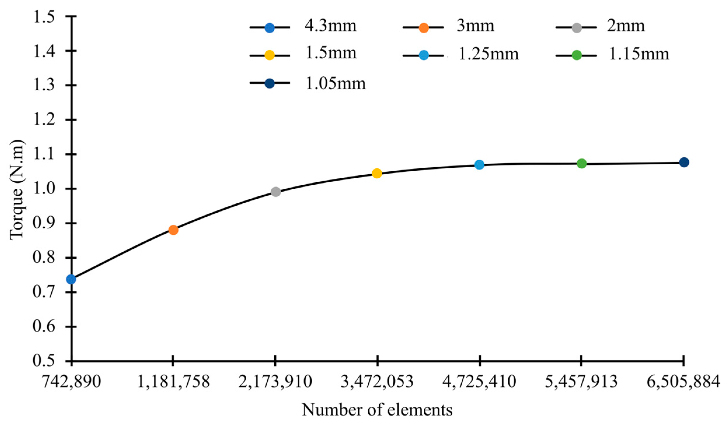
Table 2 summarizes the results of the mesh convergence study. As can be seen, increasing the fineness of the mesh typically improves its quality but increases the total number of elements, which also significantly increases the computational time.
Table 2. Grid convergence study.
Blade Element Size (mm)Number of ElementsAverage OrthogonalAverage SkewnessAerodynamic Torque (N.m)
4.3 mm742,8900.7170.2450.738
3 mm1,181,7580.7430.2290.881
2 mm2,173,9100.7890.1970.989
1.5 mm3,472,0530.8140.1791.044
1.25 mm4,725,4100.8240.171.069
1.15 mm5,457,9130.8270.1681.072
1.05 mm6,505,8840.8330.1631.076
In Figure 5, the convergence study in terms of the aerodynamic torque is illustrated. The torque starts to converge at a mesh size of 1.5 mm. A slight difference of 4.9% is observed in the aerodynamic torque between the mesh refined at 1.5 mm and 1.05 mm, but an important increase in the number of elements is also obtained. As a result, with regard to the computational cost and the mesh quality, the blade surface mesh of 1.5 mm is adopted for the CFD simulations in this work.

3.2. Model Validation

The numerical results obtained from the present blade’s modelling are compared to the experimental data of Ampair300 [18]. The rotor’s rotational speed corresponding to each wind speed is taken from the manufacturer’s manual [18]. The obtained aerodynamic torque T is used to calculate the rotor generated power P using:
P = T × Ω ,
where Ω is the rotational speed of the rotor.
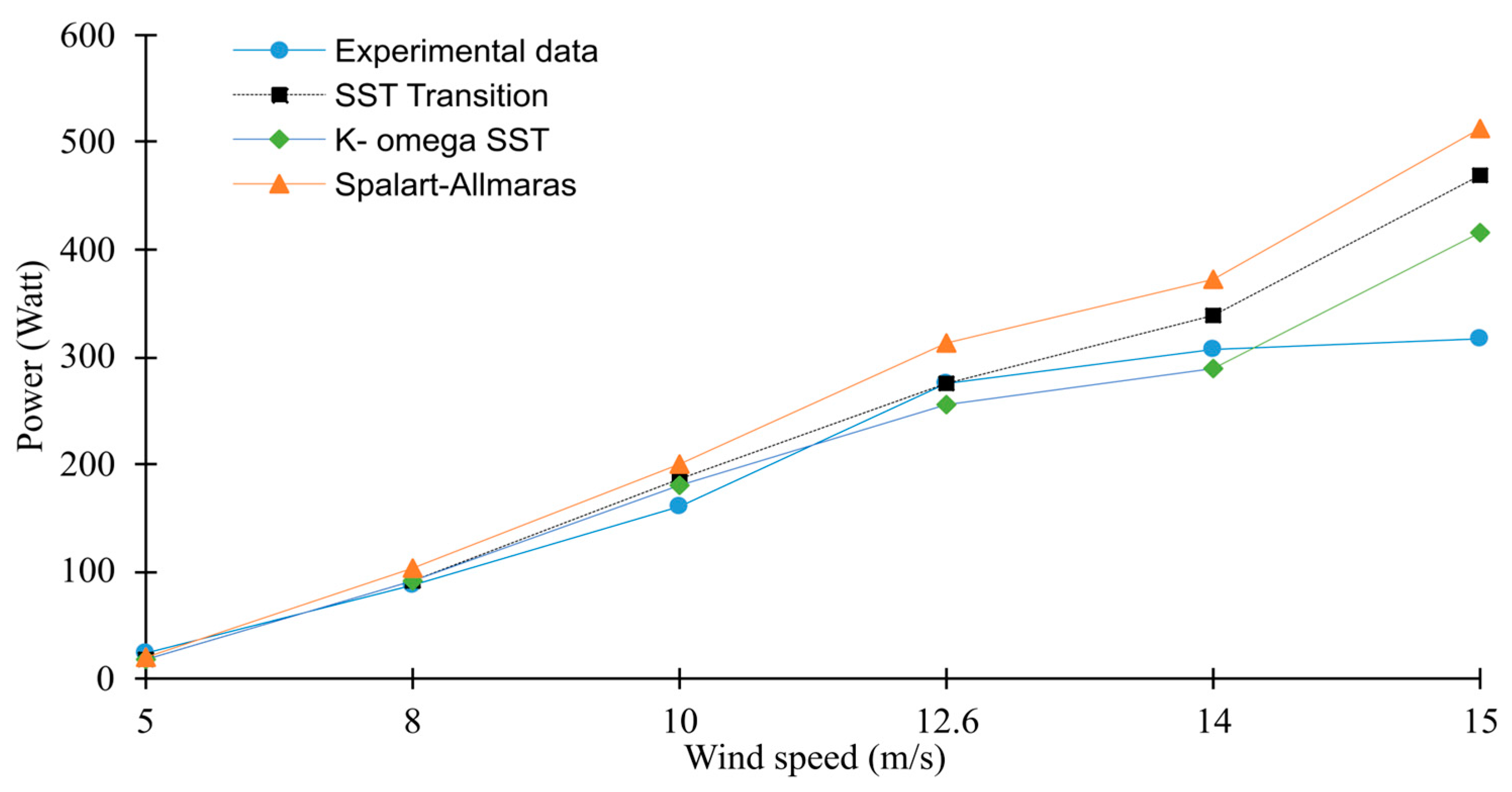
Figure 6 presents the variation in the wind turbine power with wind speeds using three different turbulence models: Spalart-Allmaras, k-ω SST and SST transition turbulence models. At low and medium wind speeds (5 m/s–10 m/s), all of the models present a reasonable agreement with the experimental data. With the increase in the wind speeds, the boundary layer (BL) of the rotor used to be laminar and is driven to turbulent flow. The laminar–turbulent transition phenomenon occurs between 10 m/s and 14 m/s. At this speed range, the SST transition shows the best prediction for the flow. Starting from 14 m/s, the present model fails to predict the rotor generated power because of the pitch control system that is activated by the manufacturer to limit the output power at wind speeds exceeding 13 m/s, as well as to avoid the high aerodynamic stresses of the wind turbine that can cause structure damage. Therefore, the transition SST model will be used in this study.

3.3. Pressure Coefficient

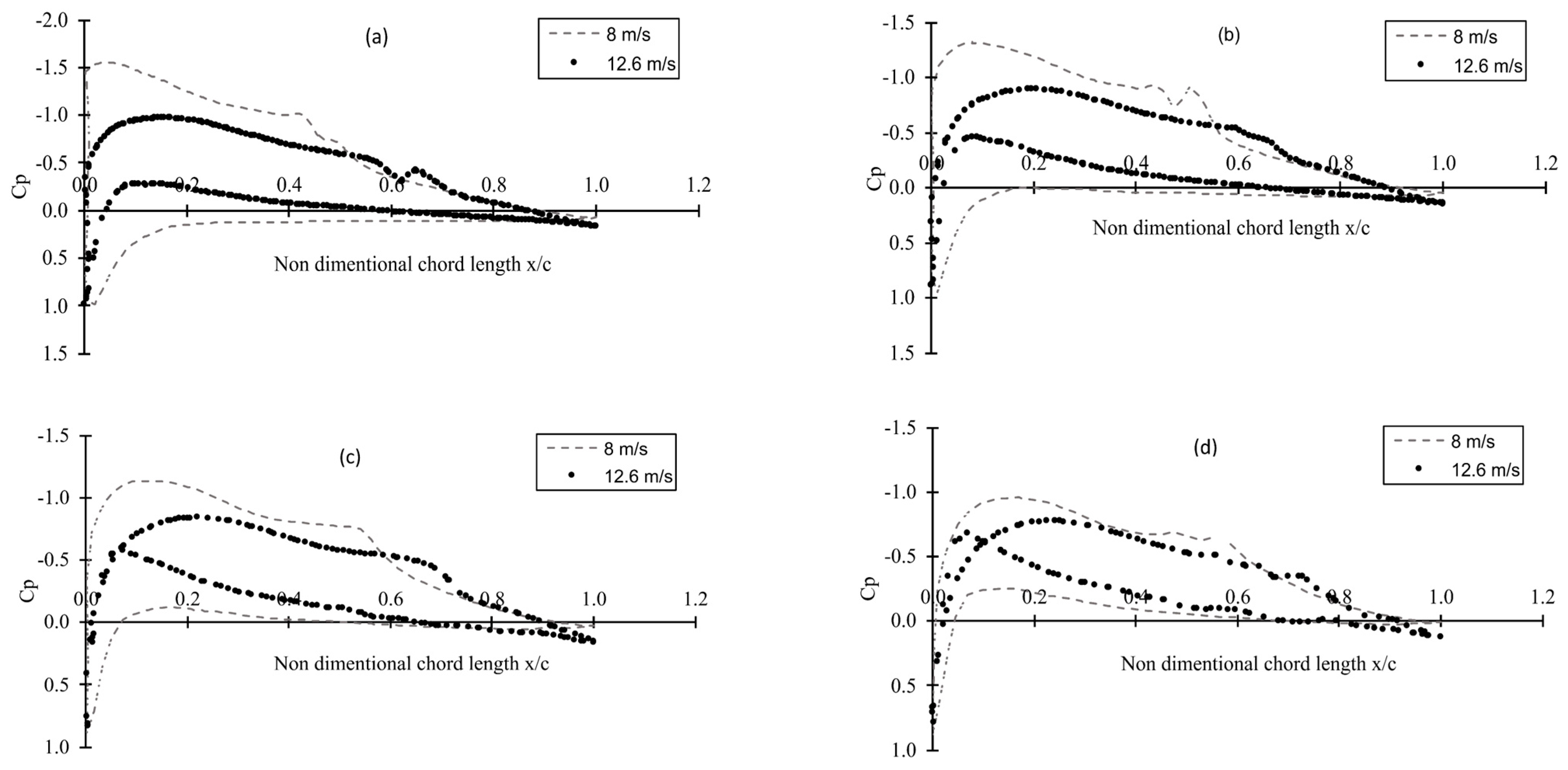
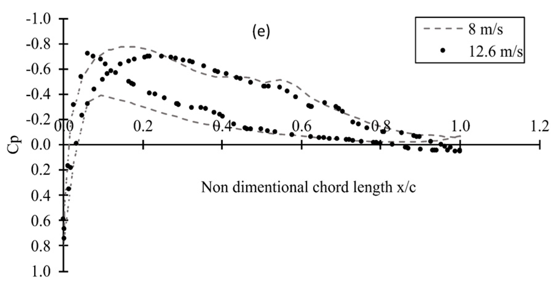
Figure 7 shows the distribution of the pressure coefficient at different important span positions and for two different operating conditions: 8 m/s and rated wind speed 12.6 m/s. The angular velocities corresponding to these wind speeds are 52.659 rad/s and 111.701 rad/s, respectively. The pressure coefficient is calculated through Equation (7) [26]:
C p = p p 0.5 ρ ( V 2 + ( r Ω ) 2 )
where p is the local pressure, p is the free stream pressure, V is the free stream wind speed, r is the local radial position, Ω is the angular velocity of the rotor and ρ is the air density.
The pressure coefficient plots show that the area enclosed by the Cp graph decreases from the leading edge to the trailing edge of the airfoil and from the root to the tip of the blade for both 8 m/s and 12 m/s. The decrease in the Cp difference indicates a decrease in the lift force as the lift force is created by the pressure difference between the upper and lower surfaces. Hence, it can be deduced that the lift force is generated near the leading edge and the maximum lift force is produced in the root region.
With the increase in the wind speed and rotational velocity, the area enclosed by Cp shrinks, indicating a decrease in the rotor efficiency due to the increase in the stresses because of the increase in the wind speed [27] and rotational velocity [28].
The laminar to turbulent transition phenomenon is one of the most important phenomena that occur at a low Reynolds number [29]. Unable to overcome the viscous effect and the adverse pressure gradient, the laminar boundary layer separates and reattaches to the airfoil surface, forming a laminar separation bubble (LSB). The plots of the pressure coefficient along the airfoil help to capture this phenomenon. As shown in Figure 7, an adverse pressure gradient is visualized in every radial position and for both operating conditions. At 8 m/s, the short laminar separation bubbles are located between 0.4 and 0.6 along the chord, whereas at 12.6 m/s, the location of the transition moves towards the trailing edge, and it occurs between the 0.55 and 0.7 chord positions. This delay in the separation can be attributed to the Coriolis force effects [30] that become much more important with the increase in the rotational velocity of the rotor. At 30.77%, 46.15%, 80.77% and 92.31%, two consecutive perturbations on the Cp profiles are observed, but only one is visible at 60.54%. An increase in the laminar separation bubble length is observed with a span-wise direction due to the decrease in the angle of attack from the root to tip regions [31]. A decrease in the Cp steepness at the transition points is observed when working at 12.6 m/s; this can be explained by the decrease in the LSB height with the increase in the wind speed [31].

3.4. Flow Field around the Blade

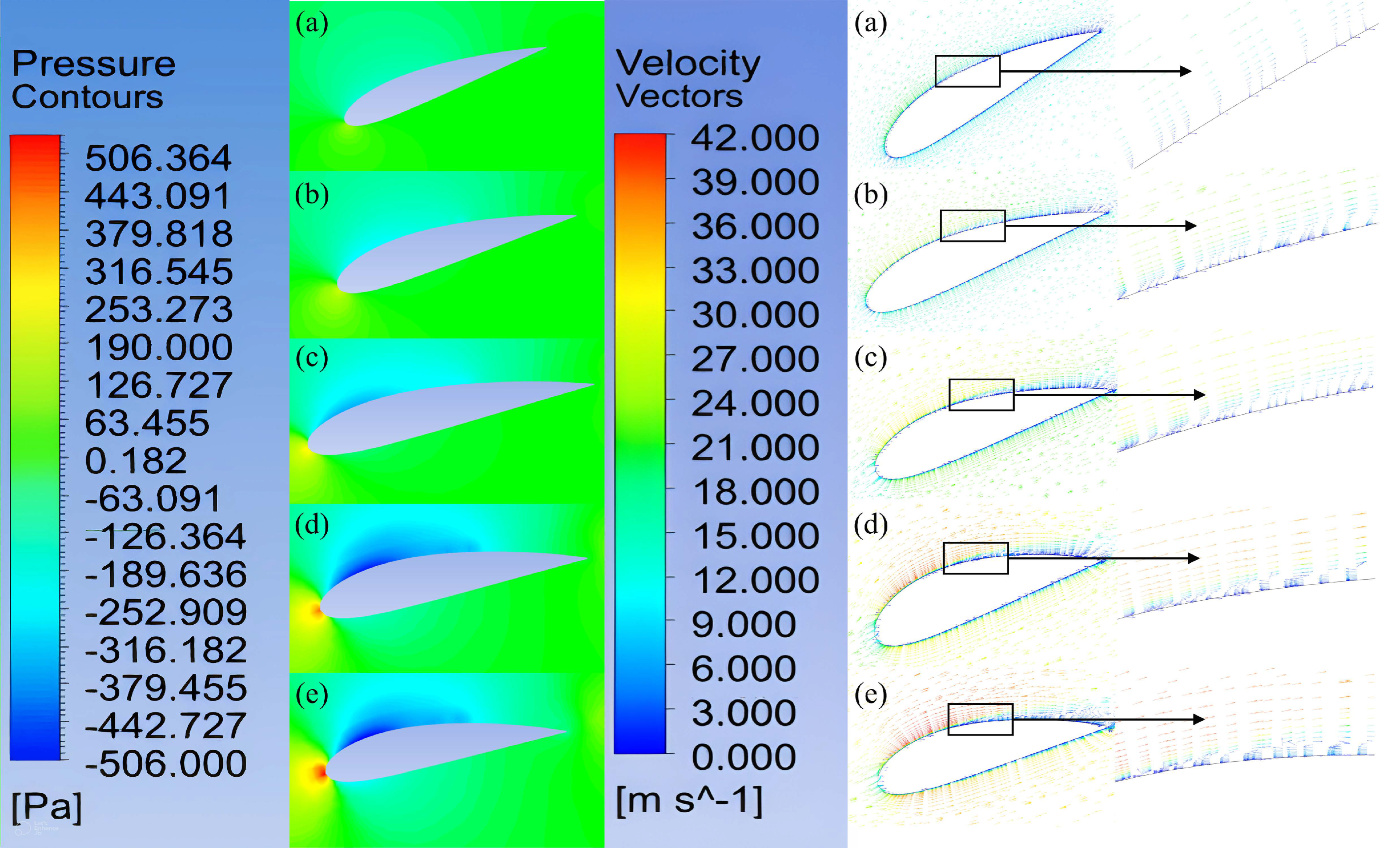
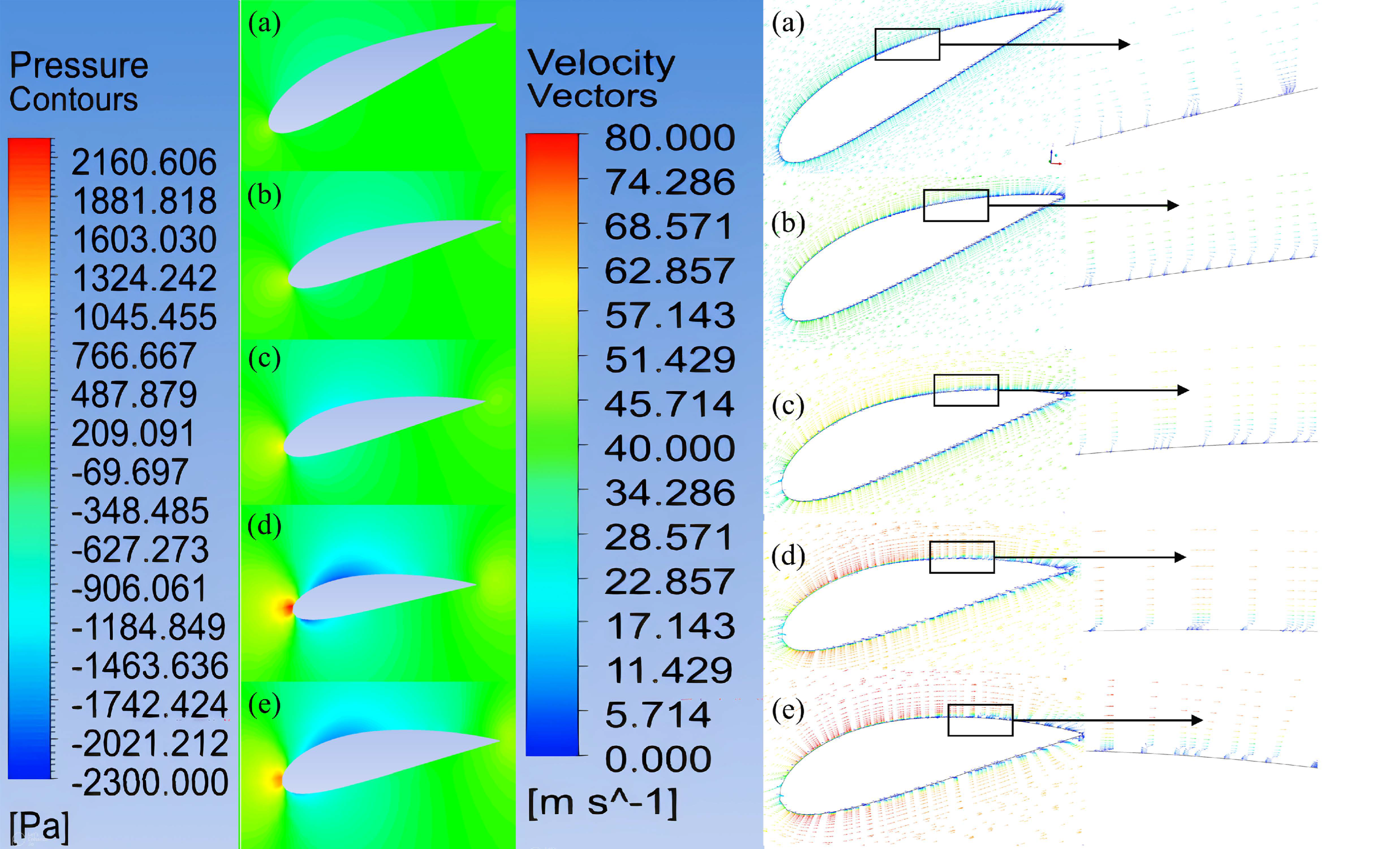
For further insight into the flow behavior around the blade, the pressure contours and relative velocity vectors of the two cases are plotted in Figure 8 and Figure 9. By comparing the contours of pressure with the vectors of velocity, it is observed that the pressure decreases when the flow accelerates. Hence, the pressure coefficient in Figure 7 is reduced rapidly to zero and takes negative values in the upper surface of the airfoil. At the lower surface, the flow slows down, so the pressure increases; as a result, the pressure coefficient difference decreases. These results agree well with Bernoulli’s principle.
The stagnation point moves up toward the trailing edge from the root to the blade’s tip. This can be explained by the variation of the angle of attack along the blade [32]. By approaching the tip, the velocity at this point used to be zero due to the flow acceleration caused by the circulation around the airfoil [33].
The velocity vectors in Figure 8 and Figure 9 illustrate the laminar–turbulent transition phenomenon on the upper surface of the airfoil. A recirculating flow is observed at the points where the Cp distribution is perturbed. In all of the radial positions, with the exception of the 61.54% span, the Cp slope shows the presence of two consecutive perturbations: a wide perturbation and a narrow perturbation. By comparing the pressure coefficient slope and velocity vectors, it is assumed that the perturbations of the Cp slope indicate transition occurrence; the flow reverses the direction and pushes the laminar layer to leave the airfoil surface. Due to the high resistance of the turbulent boundary layer flow against separation, the fluid is often attached after the transition phenomenon. Meanwhile, the presence of the second disturbance shows that the flow tries to reattach but fails to overcome the strong negative pressure gradient and the separation continues and sometimes increases before the flow reattaches to the airfoil surface.
At 30.77%, 46.15% and 61.54%, the velocity vectors show a reattachment of the laminar separated layer for both operating conditions. Whereas, at the 80.77% and 91% radial positions, the flow difficultly reattaches, a small recirculation zone is observed after the transition point and continues to flow towards the trailing edge. A delay in the separation point is recognized when operating at 12.6 m/s because of Coriolis force effects [30]. An abrupt increase in the thickness of the attached turbulent boundary layer is observed at 8 m/s in comparison with its evolution at 12.6 m/s; this agrees with the results found in [34], assuming that the turbulent boundary layer thickness decreases due to the wind speed increase.

3.5. TSR Effects

In the present work, the blade is designed using the BEM theory for a tip speed ratio of 5. In this section, the effects of the TSR on the wind turbine performance are analyzed. The study is conducted for a wind speed of 8 m/s. The power coefficient is calculated using:
C P = P 0.5 ρ V 3 π R 2 ,
where P is the calculated power from different simulations.
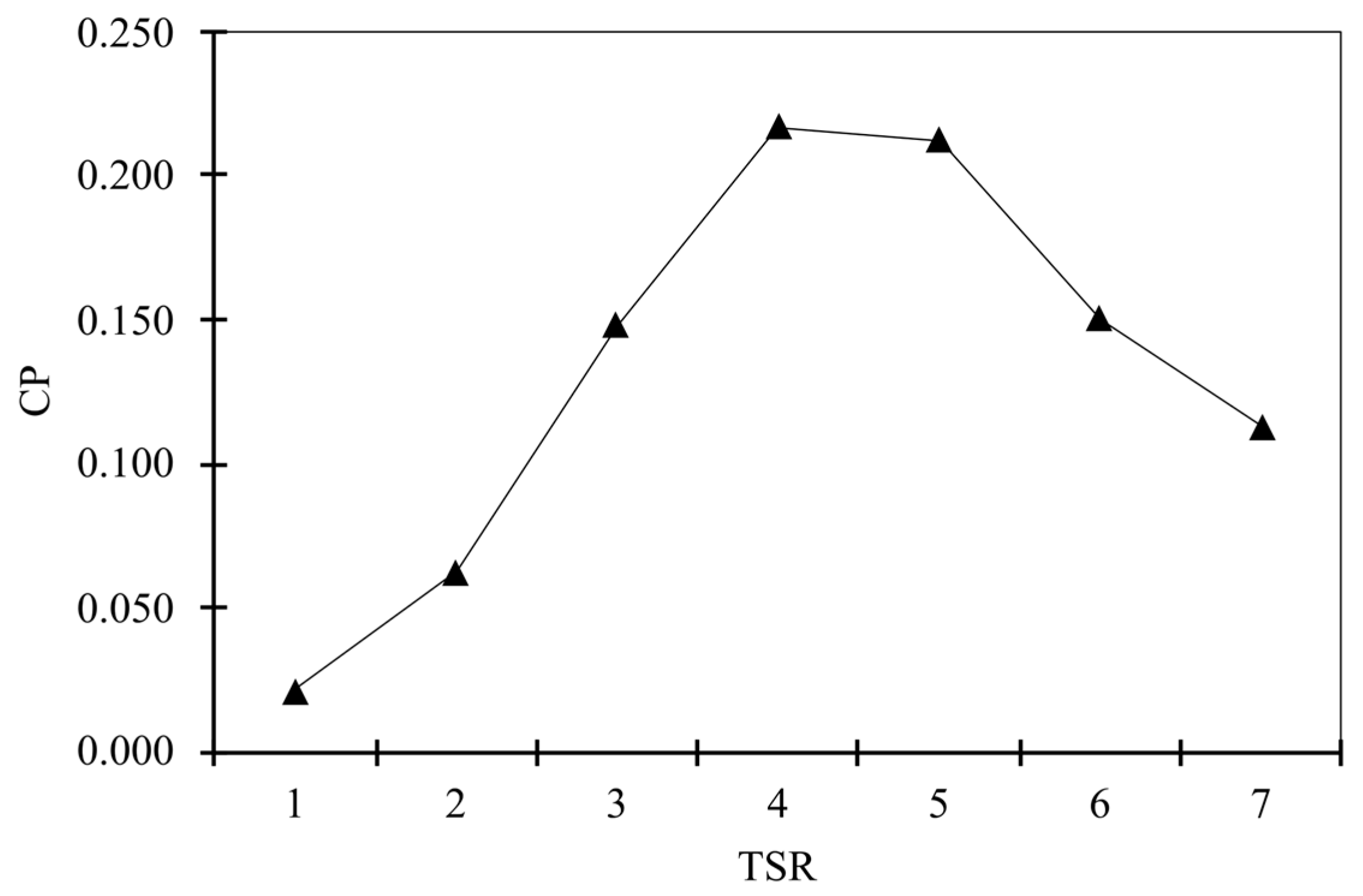
Figure 10 depicts the variation in the power coefficient CP of the present wind turbine with the tip speed ratio λ. At low TSR values, the efficiency is found to be inevitably low because, at this condition, the turbine rotates slowly so that all the wind passes through the blades without a transfer of power. The maximum power coefficient of 0.217 was obtained at a TSR of 4. This finding agrees with the results of [24], assuming that at low Reynolds numbers, the optimal TSR is between 4 and 7. After passing λ = 4, the performance of this blade decreases slowly, maintaining a quasi-high performance until λ = 6. Hence, it can be understood that, even at a high rotational speed, this blade works quite well.
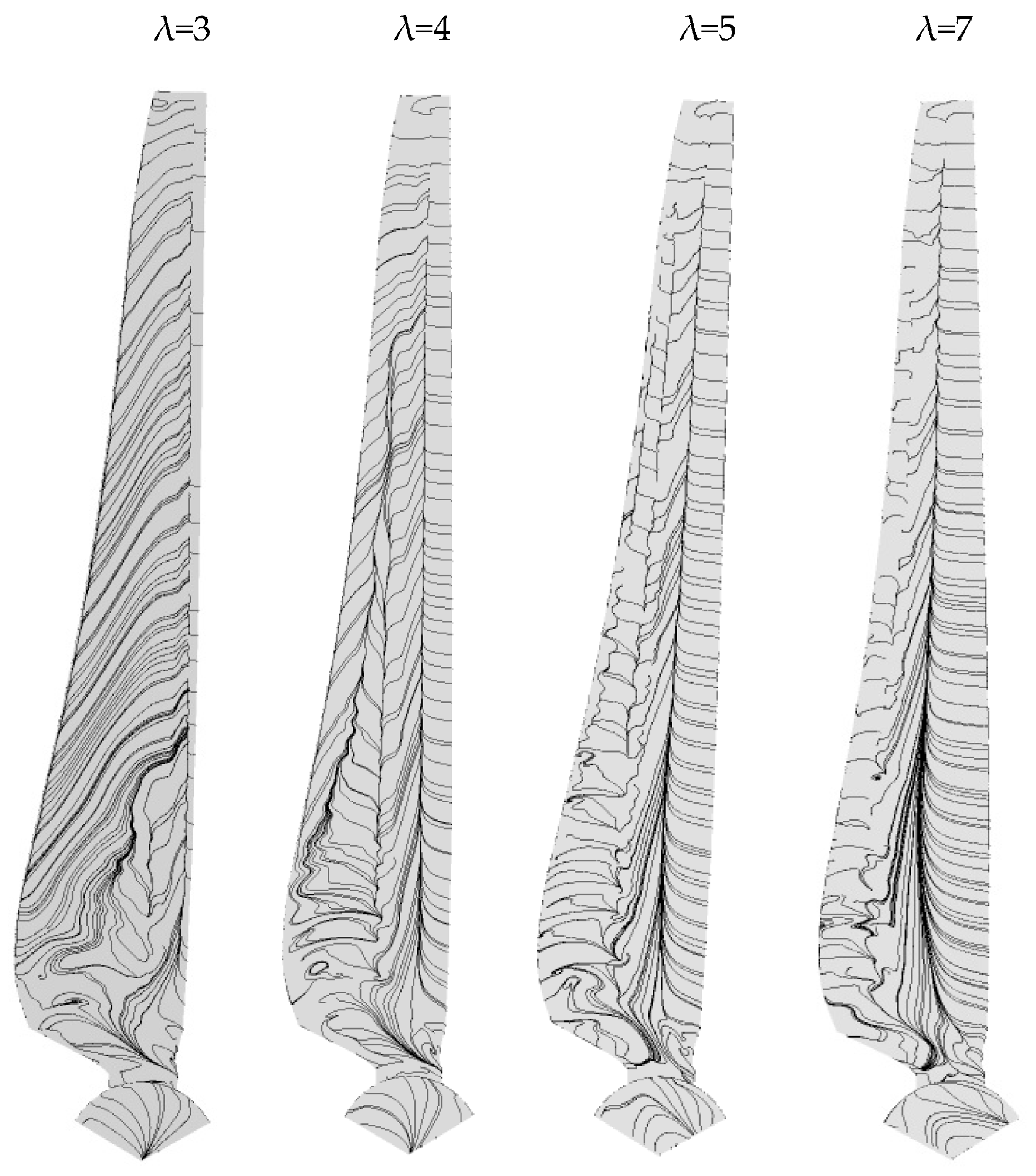
In order to study the effect of the λ on the flow behavior on the blade, the friction lines on the suction side of the blade are plotted in Figure 11. At λ = 3, the flow remains completely detached from the blade surface, with only a small attached flow zone near the leading edge along the blade. At λ = 4, where the turbine provides the maximum power along 60% of the blade, the flow is affected by the transition phenomenon; after the flow reattachment, a separation occurs at the last quarter of the blade chord and spreads towards the trailing edge. Between 60% and 90% of the blade, only one separation occurs at the first quarter of the chord. Up to 90% of the blade, the flow is fully attached. At λ = 5, the designed TSR, the transition zone and the second separation line are pushed towards the trailing edge in comparison with λ = 4. In contrast to the previous case, the transition phenomenon continues to appear until 0.9 R. Then, the flow is completely attached in the rest of the blade. At λ = 7, the transition phenomenon was observed until 75% of the blade, without a second separation after the flow reattachment. Starting from 75% of the blade, the flow becomes completely attached. A decrease in the transition zone was observed in this case in comparison with the other TSR values. This indicates that most of the flow was attached to the blade surface.
In summary, the TSR variation has important effects on the flow behavior on the blade. Due to the increase in the TSR, the Coriolis forces acting in the direction of the chord [30] become important, leading to a delay in the transition and separation phenomena. The transition zone limited by the separation line and reattachment line is reduced with the increase in the λ. The areas of separated flow on the blade surface are thinned with the rise in the TSR.
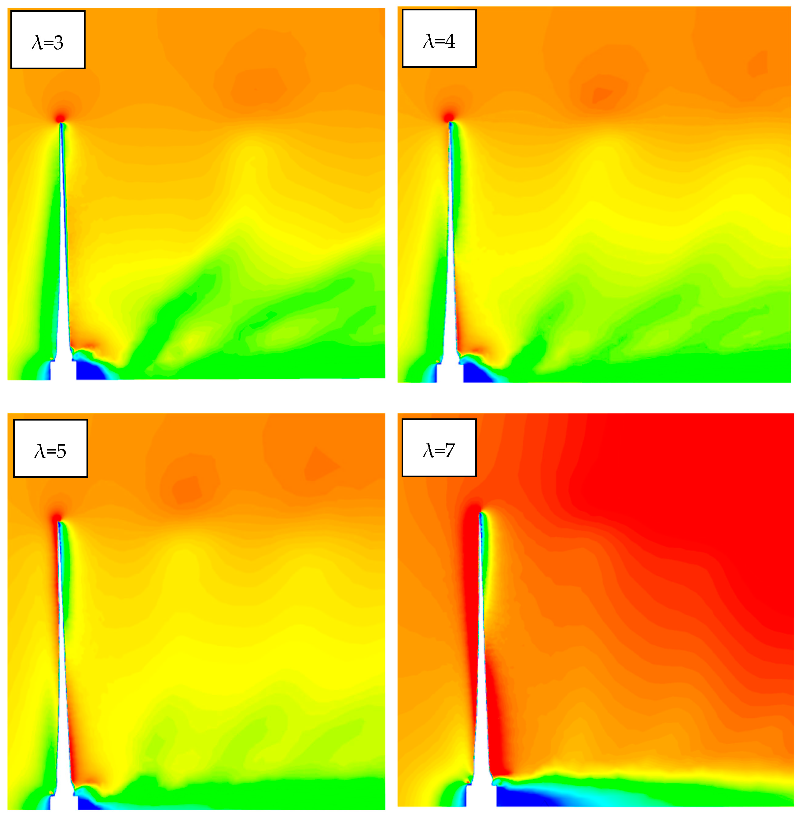
Next, the contours of the streamwise velocity W are plotted in Figure 12 in order to analyze the effects of the TSR on the wind turbine near the wake. It is observed that the wake expansion is slightly reduced from λ = 4 in comparison to the other TSRs because less energy is extracted by the rotor in these cases. The tip vortices are clearly visualized at TSRs of 3, 4 and 5; the distance between them can be observed as becoming narrow with the increase in the TSR values. At λ = 7, the tip vortices are not separated anymore but are included in a vortex sheet. The blockage phenomenon caused by the rotor hub becomes more important at high TSR values.

3.6. Pitch Angle Effects

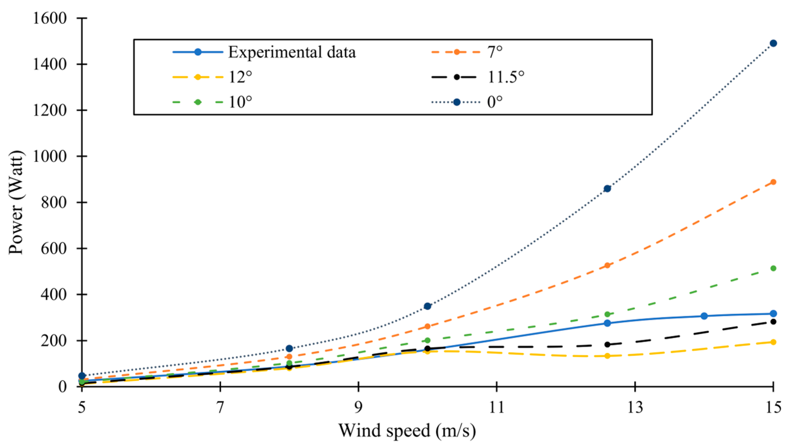
At the designed tip speed ratio (λ = 5), the effects of the pitch angle on the wind turbine performances in terms of the generated power are shown in Figure 13. The decrease in the pitch angle decreases the power at different wind speeds. The maximum generated power is recorded at a pitch angle of 0°.
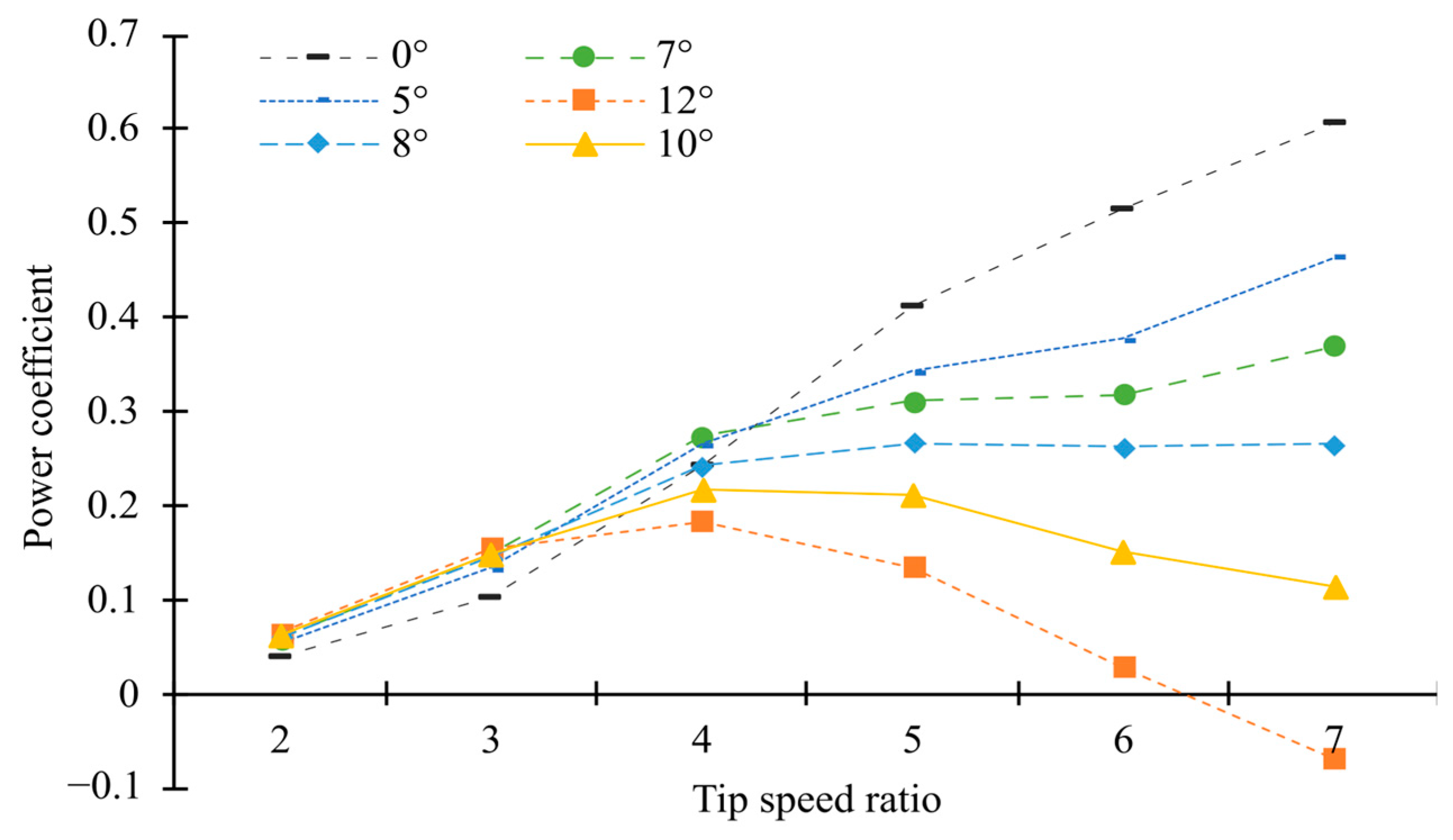
For a fixed wind speed of 8 m/s, the effects of the pitch angle on the wind turbine performances for various tip speed ratios are reported in Figure 14. The CP graphs of the 10° and 12° pitch angles reach a maximum value at a TSR of 4 and then decrease. In contrast, the trends of the other pitch angles keep increasing even at high TSRs, as well as recording important power coefficients. When the tip speed ratio is between 2 and 3, the power coefficient increases with the increase in the pitch angle. Meanwhile, when λ ≥ 5, the decrease in the blade pitch angle improves the turbine efficiency. In this range of TSRs, the highest values of power coefficients are recorded at a pitch angle of 0°; the maximum efficiency of 0.6 is obtained at a tip speed ratio of 7. When the TSR is equal to 4, the optimum power coefficient is obtained at a pitch angle of 7°.
In light of these results, it can be concluded that at low wind speeds [5 m/s, 9 m/s] and at a range of TSR greater than 4, the new designed wind turbine with a fixed pitch angle of 0° operates more efficiently than Ampair300.

4. Conclusions

The newly designed wind turbine aerodynamic characteristics were analyzed numerically using the Ansys Fluent solver for solving the incompressible, steady Reynolds Average Navier-Stocks equations. The model was validated by comparing the calculated power at different wind speeds with the experimental data of Ampair300. The comparison between the experiments showed a general good agreement at low and medium wind speeds. The conclusions of this study are presented below:
  • The transition SST turbulence model was found to be the most appropriate turbulence model for predicting the performance and flow behavior.
  • The laminar–turbulent transition phenomenon was found to be important in the blade’s root region at different rotational and wind speeds. The length of the Laminar Separation Bubble (LSB) increases with the span-wise direction, whereas the height of the LSB decreases with the increase in the wind speed.
  • At 8 m/s wind speed, the maximum power coefficient of 0.22 was recorded at a TSR of 4. The increase in the TSR leads to a delay in the transition and separation phenomena. On the blade surface, the areas of separated flow zones decrease with the rise in TSR.
  • At 8 m/s, the decrease in the pitch angle reduced the blade efficiency at low TSRs. This result was reversed at high TSRs, and the maximum power coefficient of 0.6 was obtained at a pitch angle of 0° when operating at a TSR of 7. At the medium value of TSR (λ = 4), the variation in the efficiency was found to be non-linear with the pitch angles.
  • At 8 m/s, the newly designed wind turbine with a pitch angle of 0° operates more efficiently than Ampair300 at TSRs greater than 4.

Author Contributions

Conceptualization, S.Y.; Investigation, S.Y.; Methodology, S.Y.; Project administration, A.E.; Software, S.Y.; Supervision, A.E.; Writing—original draft, S.Y. All authors have read and agreed to the published version of the manuscript.

Funding

This research received no external funding.

Data Availability Statement

Not applicable.

Conflicts of Interest

The authors declare no conflict of interest.

References

  1. Short-Term Energy Outlook—U.S. Energy Information Administration (EIA). Available online: https://www.eia.gov/outlooks/steo/report/global_oil.php (accessed on 15 June 2022).
  2. U.S. Energy Information Administration. International Energy Outlook 2016; Office of Energy Analysis U.S. Department of Energy: Washington, DC, USA, 2016.
  3. Gökmen, A.; Temiz, D. The Importance and Impact of Fossil and Renewable Energy Sources in Turkey on Business and the Economy. Energy Sources Part B Econ. Plan. Policy 2015, 10, 14–20. [Google Scholar] [CrossRef]
  4. The Socioeconomic Impacts of Wind Energy in the Context of the Energy Transition I Siemens Gamesa I KPMG. Available online: https://www.siemensgamesa.com/explore/journal/socioeconomic-report-wind-energy-2019 (accessed on 8 July 2022).
  5. International Renewable Energy Agency. Wind Energy. Available online: https://www.irena.org/Energy-Transition/Technology/Wind-energy (accessed on 22 July 2022).
  6. GWEC. Global Wind Report 2022; Global Wind Energy Council: Brussels, Belgium, 2022. [Google Scholar]
  7. Runchal, A. Brian Spalding: CFD & Reality A Personal Recollection. J. Frankl. Inst. 2014, 351, 65–87. [Google Scholar] [CrossRef]
  8. Iranzo, A. CFD Applications in Energy Engineering Research and Simulation: An Introduction to Published Reviews. Processes 2019, 7, 883. [Google Scholar] [CrossRef]
  9. Jonathon, S.; Sibuet Watters, C.; Masson, C. CFD in Wind Energy: The Virtual, Multiscale Wind Tunnel. Energies 2010, 3, 989–1013. [Google Scholar] [CrossRef] [Green Version]
  10. Kumar Gupta, R.; Warudkar, V.; Purohit, R.; Singh Rajpurohit, S. Modeling and Aerodynamic Analysis of Small Scale, Mixed Airfoil Horizontal Axis Wind Turbine Blade. Mater. Today Proc. 2017, 4, 5370–5384. [Google Scholar] [CrossRef]
  11. Hasan, M.; El-Shahat, A.; Rahman, M. Performance Investigation of Three Combined Airfoils Bladed Small Scale Horizontal Axis Wind Turbine by BEM and CFD Analysis. J. Power Energy Eng. 2017, 5, 14–27. [Google Scholar] [CrossRef] [Green Version]
  12. Muhsen, H.; Al-Kouz, W.; Khan, W. Small Wind Turbine Blade Design and Optimization. Symmetry 2020, 12, 18. [Google Scholar] [CrossRef] [Green Version]
  13. Yang, K. Geometry Design Optimization of a Wind Turbine Blade Considering Effects on Aerodynamic Performance by Linearization. Energies 2020, 13, 2320. [Google Scholar] [CrossRef]
  14. Plaza, B.; Bardera, R.; Visiedo, S. Comparison of BEM and CFD Results for MEXICO Rotor Aerodynamics. J. Wind. Eng. Ind. Aerodyn. 2015, 145, 115–122. [Google Scholar] [CrossRef]
  15. Bangga, G. Comparison of Blade Element Method and CFD Simulations of a 10 MW Wind Turbine. Fluids 2018, 3, 73. [Google Scholar] [CrossRef] [Green Version]
  16. Keerthana, M.; Sriramkrishnan, M.; Velayutham, T.; Abraham, A.; Rajan, S.S.; Parammasivam, K.M. Aerodynamic analysis of a small horizontal axis wind turbine using CFD. J. Wind. Eng. 2012, 9, 14–28. [Google Scholar]
  17. Khlaifat, N.; Altaee, A.; Zhou, J.; Huang, Y.; Braytee, A. Optimization of a Small Wind Turbine for a Rural Area: A Case Study of Deniliquin, New South Wales, Australia. Energies 2020, 13, 2292. [Google Scholar] [CrossRef]
  18. Ampair_300_Manual.Pdf. Available online: https://www.energymatters.com.au/images/ampair/Ampair_300_manual.pdf (accessed on 28 January 2022).
  19. Younoussi, S.; Ettaouil, A. Design and Optimization of a Small Horizontal Axis Wind Turbine Using BEM Theory and Tip Loss Corrections. E3S Web Conf. 2021, 294, 01003. [Google Scholar] [CrossRef]
  20. Ahmad, T.; Plee, S.L.; Myers, J.P. Fluent Theory Guide; ANSYS Inc.: Canonsburg, PA, USA, 2013. [Google Scholar]
  21. Luo, J.; Gosman, A. Prediction of impeller induced flows in mixing vessels using multiple frames of reference. I. Chem. E. Symp. Ser. 1994, 136, 549–556. [Google Scholar]
  22. Spalart, P.; Allmaras, S. A One-Equation Turbulence Model for Aerodynamic Flows. In Proceedings of the 30th Aerospace Sciences Meeting and Exhibit, Reno, NV, USA, 6–9 January 1992; American Institute of Aeronautics and Astronautics: Reno, NV, USA, 1992. [Google Scholar]
  23. Menter, F.; Kuntz, M.; Langtry, R. Ten Years of Industrial Experience with the SST Turbulence Model. Turbul. Heat Mass Transf. 2003, 4, 625–632. [Google Scholar]
  24. Langtry, R.B.; Menter, F.R. Correlation-Based Transition Modeling for Unstructured Parallelized Computational Fluid Dynamics Codes. AIAA J. 2009, 47, 2894–2906. [Google Scholar] [CrossRef]
  25. Patankar, S. Numerical Heat Transfer and Fluid Flow, 1st ed.; CRC Press: Boca Raton, FL, USA, 1980; ISBN 978-0-89116-522-4. [Google Scholar] [CrossRef]
  26. Sudhamshu, A.R.; Pandey, M.C.; Sunil, N.; Satish, N.S.; Mugundhan, V.; Velamati, R.K. Numerical Study of Effect of Pitch Angle on Performance Characteristics of a HAWT. Eng. Sci. Technol. Int. J. 2016, 1, 632–641. [Google Scholar] [CrossRef] [Green Version]
  27. Huo, Q. Structural Response Analysis of Wind Turbine under Different Wind Speeds. IOP Conf. Ser. Earth Environ. Sci. 2021, 791, 012099. [Google Scholar] [CrossRef]
  28. Shi, F.; Wang, Z.; Zhang, J.; Gong, Z.; Guo, L. Influences of Wind and Rotating Speed on the Fluid-Structure Interaction Vibration for the Offshore Wind Turbine Blade. J. Vibroengineering 2019, 21, 483–497. [Google Scholar] [CrossRef] [Green Version]
  29. Genç, M.S.; Karasu, İ.; Açıkel, H.H.; Akpolat, M.T. Low Reynolds Number Flows and Transition; IntechOpen: London, UK, 2012; ISBN 978-953-51-0492-6. [Google Scholar]
  30. Shen, W.Z.; Soerensen, N. Quasi-3D Navier-Stokes Model for Rotating Airfoil. J. Comput. Phys. 1998, 150, 518–548. [Google Scholar] [CrossRef]
  31. Koca, K.; Genç, M.S.; Açıkel, H.H.; Çağdaş, M.; Bodur, T.M. Identification of Flow Phenomena over NACA 4412 Wind Turbine Airfoil at Low Reynolds Numbers and Role of Laminar Separation Bubble on Flow Evolution. Energy 2018, 144, 750–764. [Google Scholar] [CrossRef]
  32. Kang, H.; Altman, A. Generalized Empirical Airfoil Stagnation Point Location Prediction. J. Aircr. 2007, 44, 698–701. [Google Scholar] [CrossRef]
  33. Meseguer, J.; Alonso, G.; Sanz-Andrés, A.; Pérez-Grande, I. On the Circulation and the Position of the Forward Stagnation Point on Airfoils. Int. J. Mech. Eng. Educ. 2007, 35, 65–75. [Google Scholar] [CrossRef] [Green Version]
  34. Schlichting, H.; Gersten, K. Boundary-Layer Theory; McGraw-Hill: New York, NY, USA, 2017. [Google Scholar]
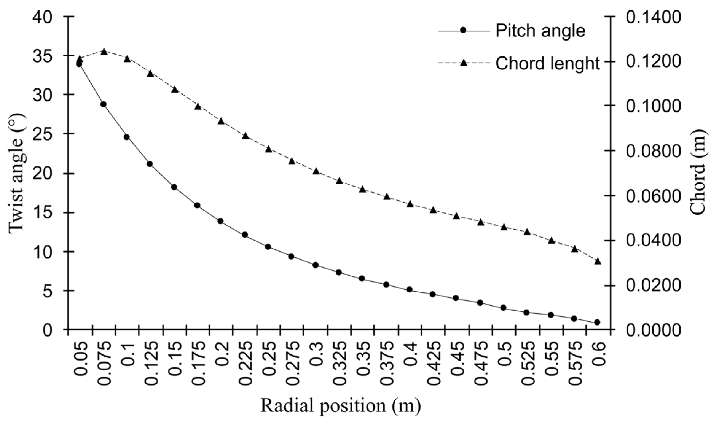
Figure 1. Chord and twist angle distribution along the blade.
Fluids 08 00192 g001
Figure 2. The optimal Blade shape: (a) Shape of the NACA4418 airfoil; (b) Twisted section airfoils; (c) Blade suction side.
Fluids 08 00192 g002
Figure 3. Computational fluid domain and boundary condition.
Fluids 08 00192 g003
Figure 4. (a) Mesh of fluid domain around the blade, (b) Tetrahedral mesh volume section, (c) Inflation of prismatic layers.
Fluids 08 00192 g004
Figure 5. Variation of the aerodynamic torque with blade.
Fluids 08 00192 g005
Figure 6. Turbine’s generated power versus wind speed at different turbulence model.
Fluids 08 00192 g006
Figure 7. Pressure coefficient Cp distribution along the chord length at different span positions: (a) 30.77% span; (b) 46.15% span; (c) 61.54% span; (d) 80.77% span; (e) 92.31%.
Fluids 08 00192 g007aFluids 08 00192 g007b
Figure 8. Pressure contours and velocity vectors distributions at 8 m/s of different radial positions: (a) 30.77% R; (b) 46.15% R; (c) 61.54% R; (d) 80.77% R; (e) 92.31% R.
Fluids 08 00192 g008
Figure 9. Pressure contours and velocity vectors distributions at 12.6 m/s of different radial positions: (a) 30.77% R; (b) 46.15% R; (c) 61.54% R; (d) 80.77% R; (e) 92.31% R.
Fluids 08 00192 g009
Figure 10. Power coefficient as function of tip speed ratio at 8 m/s.
Fluids 08 00192 g010
Figure 11. Friction lines on the suction side of the blade at different TSR values.
Fluids 08 00192 g011
Figure 12. Axial velocity in the near wake region up to 1.23R from the rotor plane.
Fluids 08 00192 g012
Figure 13. Generated power variation with wind speed at different pitch angle.
Fluids 08 00192 g013
Figure 14. Power coefficient variation with tip speed ratio at different pitch angle.
Fluids 08 00192 g014
Table 1. Characteristics of the wind turbine blade.
ParametersValues
Airfoil profileNACA4418
Designed wind speed8 m/s
Designed tip speed ratio5
αopt6.5°
R0.65 m
B3
r0.05 m
Disclaimer/Publisher’s Note: The statements, opinions and data contained in all publications are solely those of the individual author(s) and contributor(s) and not of MDPI and/or the editor(s). MDPI and/or the editor(s) disclaim responsibility for any injury to people or property resulting from any ideas, methods, instructions or products referred to in the content.