Experiments on Steam Injection into Preformed Steam Chambers of Various Shapes for Maximum Condensate Recovery

Abstract

Recently, in a previous study, we experimentally showed the existence of an optimal injected steam mass flow rate, per unit length, ${\varphi }_{opt}$, which produces the maximal recovery of condensate in a preformed steam chamber with an elliptical cross section of a horizontal semi-major axis. Mutatis mutandis, in this work, we present experimental studies in preformed steam chambers: one elliptical and the other circular. In both cases, we also found the existence of unique optimal values. These configurations try to recreate the steam condensation at a given time-lapse, as it would occur during the growth stage of the steam-assisted gravity drainage (SAGD) process: a method used in the recovery of heavy and extra-heavy oil from homogeneous reservoirs. Finding the optimal mass flow rates in the actual recovery process could be useful in the design of optimized SAGD processes.

1. Introduction

One of the most efficient thermal methods in the recovery of heavy and extra-heavy oil from reservoirs is the steam-assisted gravity drainage (SAGD) technique, which was proposed and developed by Butler et al. [1,2,3,4] in the 1980s. The SAGD process involves the injection of hot steam, at a constant pressure, into the reservoir through an horizontal upper pipe and the extraction of condensates and water/oil emulsions through a parallel pipe located beneath the injection pipe. Incidentally, there are estimations that heavy oil reserves account for more than 70% of the world’s oil reserves [5]. SAGD operations require large amounts of water (for instance, in Canada, approximately 179 million m${}^3$ of fresh water was used in 2009 for oil sands-related extractive activities [6]) along with a significant energy consumption. According to some calculations, losses represent more than 50% of the energy used in SAGD [7]. Finally, a number of efforts have been made to recover and clean the water produced in the free water phase and in the water/oil emulsion contained in the recovered fluids [8,9].

In the search for a strong reduction in the injected water and the wasted energy, it is crucial to understand the main physical mechanisms and conditions that control the efficient production of condensates [10,11,12,13,14,15]. For instance, some numerical [12,13] and experimental [14,15] studies suggest that it is possible to control the well spacing, the well placement, or the injection temperature [13] in order to optimize the oil production of heavy oil reservoirs.

By means of a simple theoretical model for a homogeneous reservoir [10], we also found an optimal (dimensionless) injected steam mass flow rate, per unit length, ${\varphi }_{opt}$, that yields the maximal recovery of condensates or water/oil emulsions at a given time-lapse. We predicted that this optimal value depends on the shape of the steam chamber edge, the physical properties of the reservoir, the operating parameters, including the well spacing and placement, and the boiling and reservoir temperatures, all of which were measured at a given time period of the growing stage of the chamber.

Following these ideas, in a recent experimental study [16], the steam injection at various mass flow rates was carried out inside a preformed steam chamber, made of glass beads occupying an elliptical space (with a horizontal semi-major axis), in an iron slab of considerable mass. By analyzing the cumulative amounts of injected steam and recovered condensates, during a short time-lapse, we identified the optimal flow rate. Then, a posteriori, we proceeded through visual and infrared images of this optimal process to track the motion of the condensation front until it reached the cold solid edge (which was assumed to represent the region where the oil behaves as a solid). Similarly, the time evolution of the temperature field was measured continuously until there was no appreciable change. This method allowed us to determine when a steady-state of the steam injection was reached for a specific injected mass flow rate.

We need to highlight that, based on field trials, the steam chamber shape evolves slowly in the time [17]. In our theoretical model [10], the (hypothetically instantaneous) knowledge of the shape of the chamber is necessary in the quantitative determination of the optimal injected mass flow rate of steam; this is the fundamental assumption in the proposal for the use of a preformed chamber in the experiments. From a theoretical point of view, the solution of the steam condensation problem at the chamber edge (of a given form), which must be computed numerically, turns out to be physically admissible only for a particular value of ${\varphi }_{opt}$, which depends on a set of dimensionless parameters.

In this work, we outline the new experimental studies related to the steam injection into preformed steam chambers of elliptical (with a vertical semi-major axis) and circular cross-sectional shapes to highlight their corresponding efficiency in the production of condensates. The use of preformed chambers embedded in highly massive slabs was conceived as an experimental setup that reproduces the main physical characteristics of the SAGD process. Moreover, in the real-life monitoring of the steam chamber formed in the oil sand layer in the lower Cretaceous McMurray formation, it was shown that the temperature distribution of the steam chamber evolved from nearly elliptical with a horizontal semi-major axis to another ellipse with a vertical semi-major axis [18].

We noticed that, in each of our ideal injection experiments, the chamber was initially dry, i.e., there was no initial water saturation, and, eventually, a steam-saturated stage was reached. However, the SAGD process is sensitive to the heterogeneity of oil sand formation, as was detected due to the presence of lean zones during the steam injection [19,20,21]. A lean zone is a zone in which water saturation is higher than 40%. The lean zone can be found in reservoirs as bottom water, top water, or pockets of water at different elevations and behaves as a thief zone during SAGD production. Field-scale studies show that a well pair is more affected by lean zones above its injector than the other cases. The high heat capacity of water, which is almost twice that of oil, when combined with high water saturation, leads to high steam demand when steam intercepts a lean zones. For this reason, the steam–oil ratio (SOR) increases and oil production decreases. When these inhomogeneities are absent, the SAGD technique is generally efficient, with steam–oil ratios in the 2 to 5 range, which means SAGD generally requires between two to five barrels of water to be converted into steam for the recovery of one barrel of crude oil. The pressure of the lean zone is another parameter that influences SOR and the bitumen rate during the SAGD operation. Lean bitumen at low pressure (lower than 1000 kPa) may require a large volume of steam to increase the pressure to that of the SAGD operation pressure.

It is important to note that, perhaps due to the seminal works of Butler [1,2,3,4], many theoretical and experimental works have reported steam injection in terms of volume flow rates (see, for instance, [7,11,14,22,23]). However, to measure gas flow using a volumetric flow meter, temperature and pressure measurement are required, along with the gas density, to convert the volumetric flow into mass flow. One of the advantages of measuring gas mass flow is that the mass does not change with the temperature or pressure. The mass flow measurement is known to offer more reliable, accurate, and more repeatable data when compared with volumetric flow methods. Consequently, our main results for gas or liquid flows will be given in terms of mass flow rates.

This work is organized as follows: In the next Section, we provide the analytical expressions that describe the shape of the chambers studied in the experiments. In addition, we briefly discuss the main physical parameters involved in the determination of the optimal recovery of the condensates. Later on, in Section 3, the experimental setup will be presented and we will discuss the evolution of the transient condensation fronts in the elliptical and circular steam chambers. Thereafter, we will report the measurements of the temperature fields in the chambers to determine the steady-state phase change temperatures, close to the steam chamber edges. In Section 4, the injected steam and the accumulated quantities of recovered condensates allows us to present, in a dimensionless form, the plots of the recovery efficiency of condensates for the elliptical and circular steam chambers. Finally, in Section 5, the main conclusions and limitations of this study will be presented.

2. Preformed Steam Chambers and Parameters Governing the Steam Flow

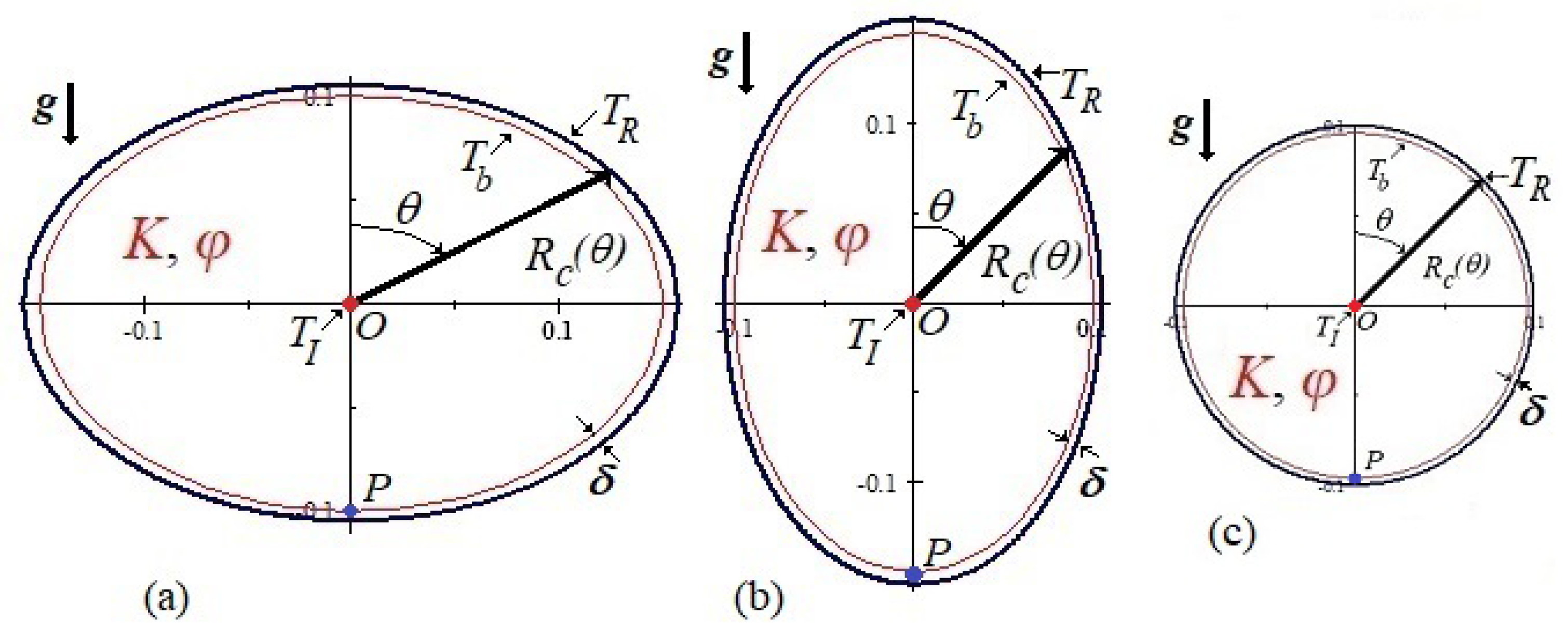
2.1. Preformed Steam Chambers

Our theoretical model focuses on the steam flow radially injected from the injection pipe into a porous steam chamber of permeability K and the recovery of the condensed water, due to gravity drainage, at the lower recovery pipe [10]. Again, we justify this approach given that, in the actual SAGD process, the injected steam displaces the oil, leading to the formation of a steam-saturated zone partially depleted of oil, i.e., the steam chamber, around the injection pipe.

In order to gain physical insights into the main mechanisms of heat and mass transfer within the steam chamber, we consider, as in the theoretical model, nearly two-dimensional preformed chambers, such as those sketched in Figure 1.

The limit of the steam chamber is the edge of the chamber, where a thin layer of mean thickness $\delta$ consisting of a water/oil emulsion, which drains by gravity towards the production pipe. Beyond this layer, there is a region where the highly viscous oil saturating the rest of the reservoir behaves as a solid. We assume, by using cylindrical coordinates, that within a given time-lapse, the chamber edge has the form $r=R_c\left(\theta \right)$, with the symmetry condition expressed as $R_c\left(\theta \right)=R_c(-\theta )$, where $0\le \theta \le \pi /2$ and $\theta$ is measured clockwise from the upper vertical axis ($\theta =0$) to the lower vertical axis ($\theta =\pi /2$).

In Figure 1, we depict the cross sections of two preformed elliptical chambers with different orientations and one preformed circular chamber, all of them centered at the origin O, where the injection pipe is also placed (red dot). In the scheme of Figure 1a, the ellipse has a horizontal semi-major axis, while the ellipse in the scheme of Figure 1b has a vertical semi-major axis. Finally, the scheme of the circular chamber is shown in Figure 1c. The generic equation describing the shape of the edges of the preformed steam chambers is

$$R_c\left(\theta \right)=\frac{ab}{{\left(a^2{cos}^2\theta +b^2{sin}^2\theta \right)}^{1/2}}.$$

(1)

The corresponding values of a and b, for each edge in Figure 1, are given in

Table 1. Values of the geometrical parameters of Equation (1).

Shape of Chamber Edge	a (m)	b (m)
Ellipse (horizontal semi-major axis)	0.157	0.105
Ellipse (vertical semi-major axis)	0.105	0.157
Circumference	0.10	0.10

. In the specific case of the circular chamber, the radius is $R=a=b=0.10$ m. We chose these edge shapes for ease of machining and, as previously mentioned, due to the actual formation of both aforementioned elliptically shaped steam chambers [18]. It is worth mentioning that, in a previous work [16], we already analyzed the steam injection into the elliptical steam chamber of Figure 1a, and it is referred to here to contrast with the new results obtained for the other two steam chamber designs, and to emphasize the importance of the shape of the steam chamber on the efficiency of the recovery of condensates.

The elliptical steam chamber of Figure 1b is materially the same as that of Figure 1a, which was manufactured in a cast iron slab with a height of $0.50$ m, a length of $0.36$ m, and thickness of $0.041$ m. To enclose the porous layer between two glass plates, the hollow elliptical space in the slab was filled with glass beads (soda lime) of diameter $d=0.6$ mm. With these data, we reported in [16] that the mean porosity is $\phi \approx 0.40$ and the permeability is $K\approx 3.55\times {10}^{-8}$ m${}^2$. These same values are assumed to be valid for the porous medium in the circular steam chamber since the same glass beads were used in this case.

To facilitate the optical and infrared visualization of the steam flow in the steam chamber, we placed plates of transparent armored glass of elliptical shapes $0.013$ m thick on each side of the chamber; thus, the chamber was $l=0.015$ m deep, which was also the length of the steam diffuser used to radially and evenly distribute the hot steam. The armored glasses were selected to prevent an explosive rupture caused by the thermal stresses and because they were subject to multiple cycles of use.

For the elliptical steam chamber, the distance between O and P was $H=0.14$ m. At O, the diffuser had an external radius of $R_I=7\times {10}^{-3}$ m, meaning that the dimensionless radius was $ϵ=R_I/H=0.05$, the radius of the orifice of recovery, which was open to the atmosphere, was the same as $R_I$. The bores drilled to embed the diffuser in the glass plate and the recovery port were machined only on the rear glass plate.

In the case of the circular steam chamber (Figure 1c), the chamber was embedded in a slab $0.51$ m high, $0.51$ m long, and $0.064$ m thick. In this case, the porous layer was enclosed between two Plexiglas plates $0.011$ m thick; hence, the chamber had a depth of $l=0.029$ m and matched the length for the steam diffuser. Here, the distance between O and P was $H=0.07$ m, and the radius of the diffuser of steam was $R_I=5\times {10}^{-3}$ m, which was the same for the recovery orifice. Consequently, now we have that $ϵ=R_I/H=0.07$.

As is shown in Figure 1, the areas of the ellipses were the same: $A_e=\pi ab=0.052$ m${}^2$ and the area of the small circumference was $A_c=\pi R^2=0.031$ m${}^2$, which means that the area of the circumference was around $0.6A_e$. Our criterion for the size of the circumference was that it could be inscribed in the ellipse.

2.2. Parameters of the Steam Flow in SAGD

Similar to our theoretical treatment [10], it was assumed that the injected steam condenses in a thin layer close to the chamber edge $r=R_c$, see Figure 1. If the condensate is mainly composed of water, then it has dynamic viscosity ${\mu }_w,$ density ${\rho }_w$ and both of them will be characterized at temperature $T_b$, which is the boiling temperature of the phase change.

The governing equations for the steady state flows of steam and condensate, valid for a short time-lapse of the SAGD process, yield several dimensionless physical parameters, whose values are directly related to the shape of the steam chamber edge, $R_c\left(\theta \right)$, and to the conditions for which the optimum mass flow rate occurs [10]. These parameters are

$$S=\frac{c_p{T}_b}{L},\frac{T_I}{T_b},ϵ=\frac{R_I}{H},\mathsf{\Pi }=\frac{{\rho }_w^{2}KgHL}{{\mu }_w{k}_e{T}_b}\frac{T_b-T_R}{T_b},$$

(2)

where $c_p$ is the steam specific heat, L is the latent heat of condensation, and $k_e$ is the effective thermal conductivity of the steam saturated medium, which will be taken according to the temperature $T_b$. Other important quantities are g: the acceleration due to gravity, and $T_I$ and $T_R$: the temperatures of the steam at injection and at the edge of the steam chamber, respectively.

The physical meaning of the dimensionless group of parameters given in (2) are discussed in [10], but in summary: S is the parameter that measures the ratio of the steam enthalpy (heat energy at a constant pressure) to the latent heat (heat released per unit mass when the substance condenses), the value of $T_I/T_b$ amounts to the ratio between the injection temperature $T_I$ with respect to the phase change temperature $T_b$, $ϵ$ is the radius of the injection pipe scaled with H, and the dimensionless parameter $\mathsf{\Pi }$ is related to the dimensionless optimal mass flow rate, per unit length, ${\varphi }_{opt}={\varphi }_{opt}^{*}/(k_e{T}_b/L)$, where ${\varphi }_{opt}^{*}$ is the dimensional optimal mass flow rate per unit length. An analysis of the relation between $\mathsf{\Pi }$ and ${\varphi }_{opt}$ establishes as $\mathsf{\Pi }$ increases, wherein ${\varphi }_{opt}$ also increases [10]. We notice in (2) that an increase in $\mathsf{\Pi }$ (and consequently an increase in ${\varphi }_{opt}$) occurs if $T_R/T_b$ decreases. In this sense, a substantial difference between $T_b$ and $T_R$ improves the condensates recovery. However, it was also found that if the injection temperature $T_I$ is large, the heat flux that reaches the condensation front from the steam leads to a decrease in ${\varphi }_{opt}$. The dimensionless condensate film thickness ${\delta }^{\prime }$ was estimated to be ${\delta }^{\prime }={\mu }_w{\varphi }^{*}/{\rho }_w^{2}gKH$, and, for the optimal case, it is ${\delta }_{opt}^{\prime }={\mu }_w{\varphi }_{opt}^{*}/{\rho }_w^{2}gKH$.

Finally, it was found theoretically and experimentally [10,16] that if the dimensionless injected flow rate is larger than ${\varphi }_{opt}$, then a fraction of the steam rapidly reaches the production pipe, without condensing inside the chamber. Conversely, if the injected flow rate is smaller than ${\varphi }_{opt}$, then a large amount of the steam condensates very rapidly and it drains to the production pipe without reaching the edge. The value of ${\varphi }_{opt}$ separates these undesirable conditions and must be given as a function of the parameters (2). Many of these claims will be supported by the current experimental results.

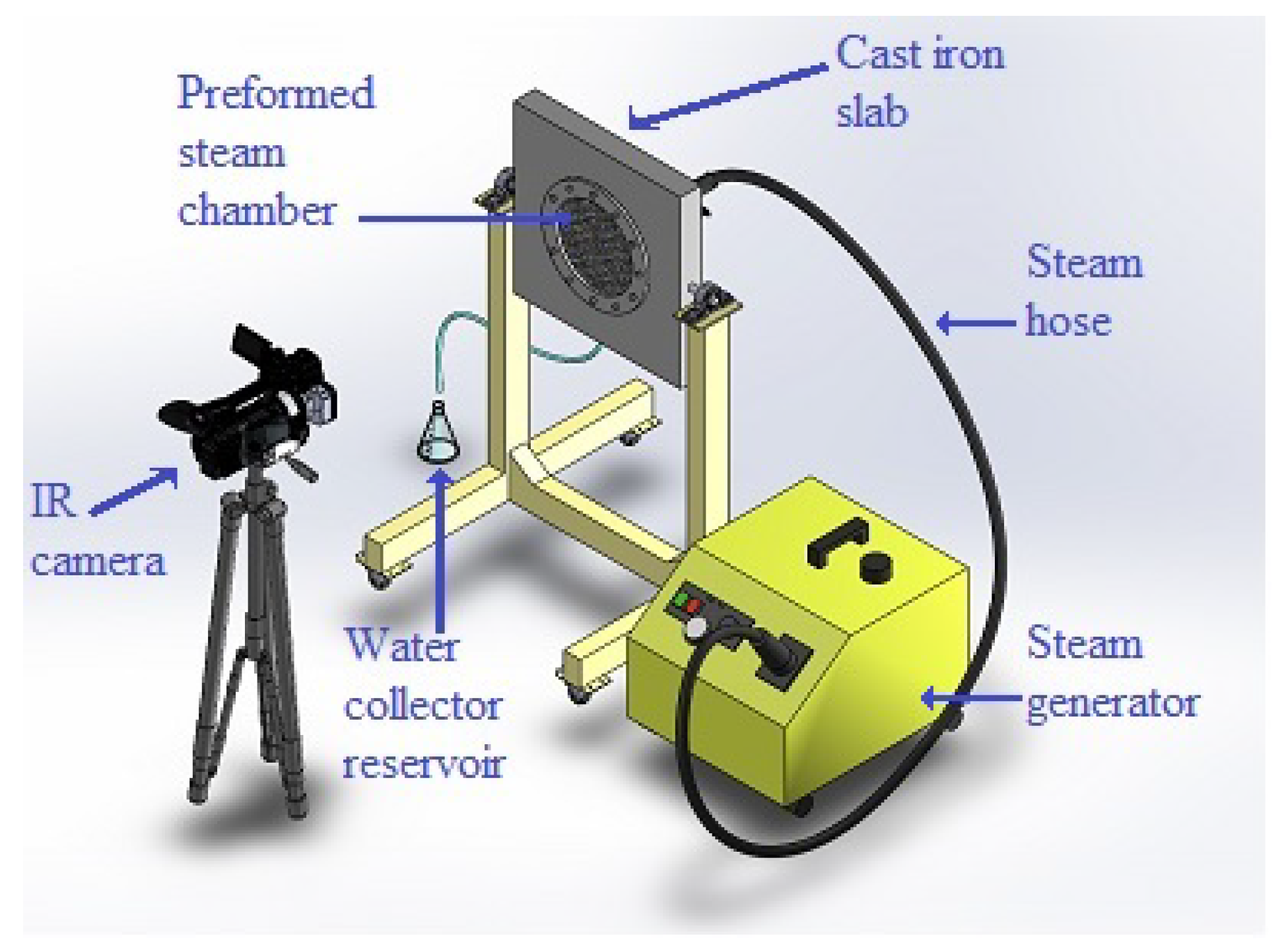
3. Experiments of Steam Injection into Elliptical and Circular Chambers

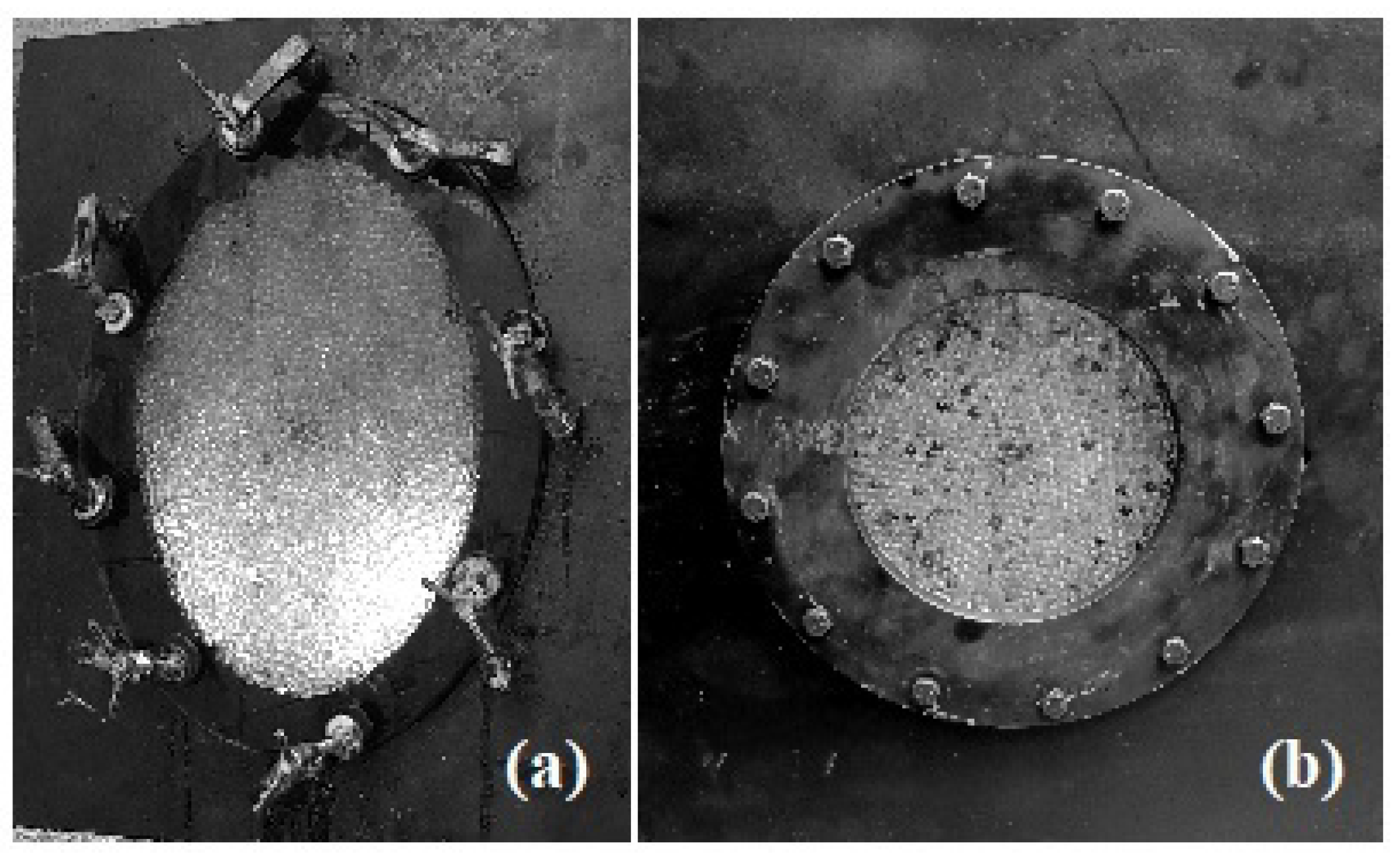
The well constraints in the experiments were that, along the injection pipe, steam is injected radially into the porous medium at pressure $p_I$ and, in the recovery pipe, the condensates, and eventually the steam, flow out. In terms of the pressure, the lower end of the chamber is close to the production pipe, and during injection, the pressure in the chamber decreases to about the pressure in the production pipe, which is the ambient pressure (in an actual reservoir, such a pressure is not very different from that of the reservoir [24]). In this stage, the spatial pressure variations in the steam chamber are small compared with the hydrostatic pressure variation in a distance of the order of the height of the steam chamber. However, the small spatial pressure variations determine the flow of steam into the chamber and the distribution of condensation flux at its boundary.

3.1. Steam Chambers

For the continuous steam injection into the preformed steam chambers, we used the same steam generator described in our previous experimental study [16]. In Figure 2, we schematically show the cast iron slab enclosing the circular steam chamber, which is mounted on a support structure and, at the rear of the chamber, the jet nozzle is connected to a radial diffuser located within the chamber. We used optic and IR cameras to visualize, in real time, the motion of fluid and the isotherms distribution whenever possible.

In the current experiments, the preformed steam chamber initially contained the air-saturated porous medium consisting of dry glass beads at room temperature $T_{room}=293.15\pm 1$ K, which was the same as that of the metallic slab. For the case when the optimal mass flow rate was determined, after the injection at different flow rates, we carefully observed through the treatment of digital images, the displacement process of the condensation front that eventually reached the edge of the chamber. After the condensate reached the edge, it drained toward the recovery pipe at the bottom. In Figure 3, we show the elliptical (Figure 3a) and circular (Figure 3b) preformed steam chambers used in the current study.

The procedure used to inject specific amounts of saturated steam was reported elsewhere [16] and was based on the method of the direct contact condensation of steam jets [25,26]. Consequently, the injected steam mass $m\left(t\right)$ was always known as was the mass flow rate $\stackrel{·}{m}=dm/dt$. Through a thermocouple located within the chamber right at the injection orifice, we found that, for all the cases, the injection temperature was $T_I=365.15\pm 1$ K; thus, the absolute injection pressure was $p_I=75.68$ kPa [27]. Later on, we report the results of the transient evolution before the flow reached a steady state, first for the elliptical steam chamber and then for the circular chamber.

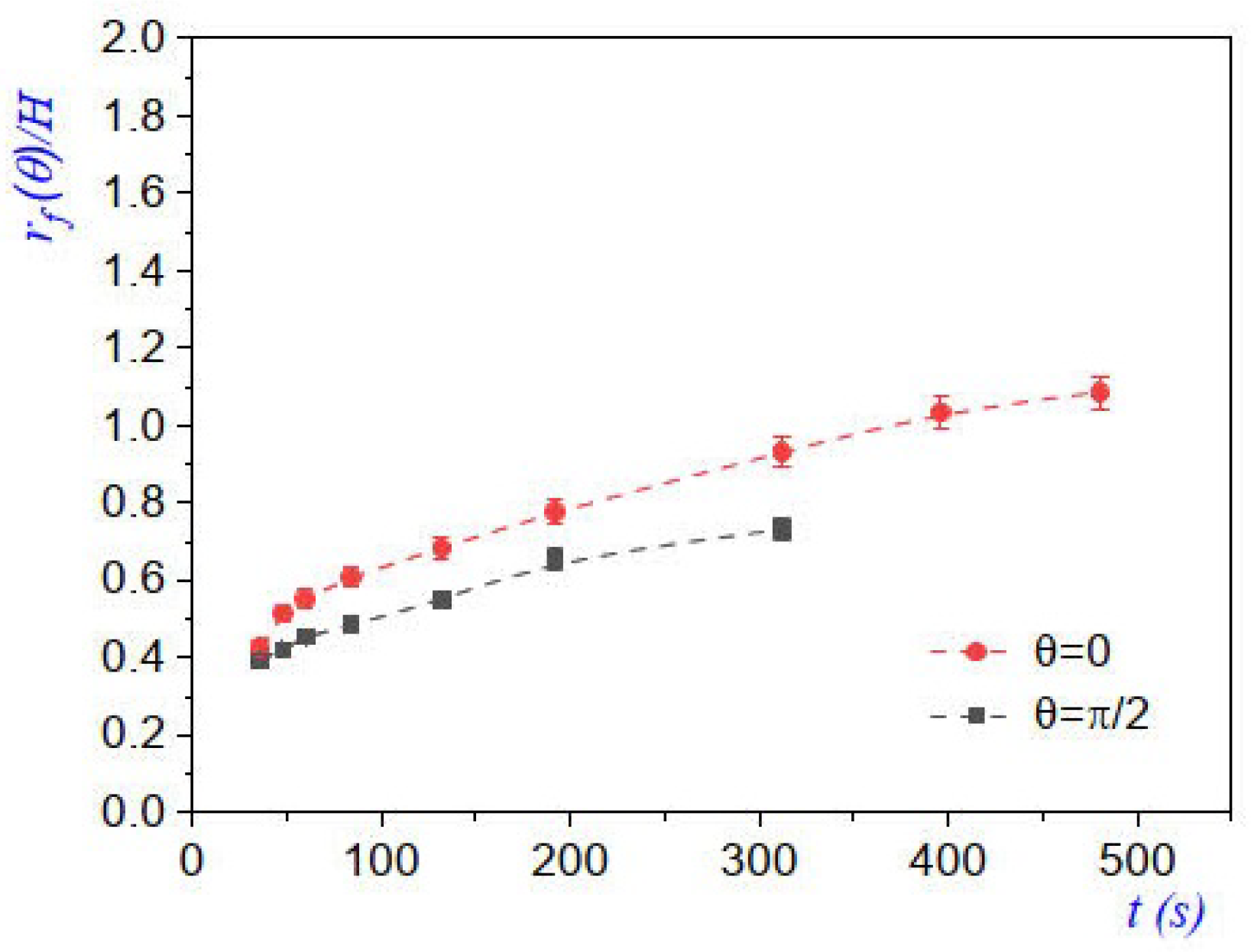
3.2. Transient Steam Flow in an Elliptical Steam Chamber

A digital image subtraction treatment was applied to photographs taken every 12 s during experiments, where the optimal steam injection ${\varphi }_{opt}^{*}$ was reached. In Figure 4, we present different stages of the evolution of the front within the elliptical steam chamber with a vertical semi-major axis. In addition, we show the evolution of the condensation front from the central diffuser up to the chamber edge. In Figure 4a, the advancement of the condensation front was nearly radial, and in Figure 4c,d, we observed that the condensation front first reached the regions close to $\theta =\pi /2$ and $\theta =3\pi /2$, and finally, the front reached the top ($\theta =0$) and lower ($\theta =\pi$) regions.

Neither the evolution of the condensation front nor the transient evolution of the temperature distribution were considered in our theoretical model; however, both aspects became relevant in the experiments because they involve the thermalization process of the preformed steam chamber. In the plot of Figure 5, we show the time evolution of the dimensionless front $r_f\left(\theta \right)/H$ along the horizontal ($\theta =\pi /2$) and vertical ($\theta =0$) axes. The curve fits for both cases correspond to power laws of the form $r_f/H\sim t^n$, where $n=0.29\pm 0.01$ if $\theta =0$ and $n=0.34\pm 0.01$ if $\theta =\pi /2$. Moreover, in the same figure, it is observed that the rate of change of $r_f(\theta =0)/H$ was larger than $r_f(\theta =\pi /2)/H$, due to the influence of the buoyancy of steam. In contrast, when a hot liquid is injected radially into a similar geometry at a constant flow rate, q, the Darcy velocity of the front close to the injection pipe, $v_r$, evolves as $v_r=d{r}_f/dt=q/2\pi r_f$, which yields that $r_f/H\sim t^{0.5}$ [28].

In addition, the time-dependent temperature distributions in the preformed steam chamber during the steam injection (see Figure 6) were obtained using an infrared camera: model FLIR SC660, which had a high performance infrared system within the long-wave spectral range: 7.5–13 $\mathsf{\mu }$m. It should be mentioned that the temperature scales in the thermographies Figure 6a–d needed to be corrected with surface radiation exchange methods [29]. This was performed knowing the thickness and the physical properties (density and refractive index values) of the observation window, which was made from soda lime glass and allowed the visualization of the steam flow and temperature distributions.

In Figure 7, we show the plot of the dimensionless temperature distribution $T\left(\theta =\pi /2\right)/T_b$ along $r(\theta =\pi /2)/H$, for two different time instants. In said plot, data were collected from the termographies of Figure 6c,d, which were 340 s apart; however, they are very similar to each other. Accordingly, the correction of the temperature values, which was necessary due to the radiation exchange mentioned earlier, was carried out, resulting in the data presented in the plot. For completeness, the data measured and used in the construction of the plot in Figure 7 were $T_b\approx 350.45\pm 1$ K (defined as the temperature value where the slope suddenly changes), $T_I=365.15\pm 1$ K, and $H=0.14$ m. Notice that the close similarity between the dimensionless temperature distributions in said plot provides evidence of a steady-state regime being reached. The mean temperature ${\left(T_R/T_b\right)}_{mean}=0.906$ was determined at the chamber edge $r(\theta =\pi /2)/H=\left(a/H\right)=0.75$ where a, which is given in Table 1.

3.3. Transient Steam Flow in a Circular Steam Chamber

We now present experimental results similar to those in the previous subsection but for circular cross sections; all data were obtained for the corresponding optimal injected mass flow of steam, ${\varphi }_{opt}^{*}$. In Figure 8, we show the evolution plot of the condensation front as it approached the chamber edge. In Figure 9, we present the plot of the evolution along the vertical line $r(\theta =0)/H$ (dashed red curve) and along the horizontal line $r(\theta =\pi /2)/H$ (dashed black curve). Now, the exponents of the power law $r_f/H\sim t^n$ are $n=0.51\pm 0.02$ if $\theta =0$ and $n=0.46\pm 0.02$ if $\theta =\pi /2$. These exponents indicate, as can be seen in Figure 8, that the initial fronts were nearly circular and behaved approximately according to the power law for hot water radial injection [28].

Following the study of the thermalization of the preformed circular steam chamber, we provide four thermographies for the indicated time instants in Figure 10. Through Figure 10c,d, we notice that, at the bottom, a water accumulation (liquid pool) appeared as a consequence of the recovery orifice (black dots in said figures), located 0.03 m above the lower edge of the chamber. It is apparent that similar cases could occur in actual SAGD processes, similar to the lean zone discussed in the Introduction. Therefore, the experimental visualization of this case is of interest [30].

From Figure 10c,d, the existence of several horizontal isotherms in the confined aquifer is evident, and these had a double effect: First, they release heat onto the iron slab by conduction at temperatures lower than $T_b$; second, the condensate coming from the upper parts of the chamber edge must go through a liquid region (close to the red isotherm) where the shear stress limits its speed, thus causing the flow rate at the recovery orifice to drop.

Finally, two temperature measurements along the horizontal line $r(\theta =\pi /2)$ were taken 430 s apart (see Figure 11). The corresponding boiling temperatures were $T_b=358.4\pm 1$ K for the dashed black curve and $T_b=360.4\pm 1$ K for the dashed red curve. It is possible that the slight temperature reduction at $t=1080$ s could have been caused by the continuous heat transfer to the solid slab, as can be observed in Figure 10d.

4. Optimal Injected Mass Flow Rates in the Steam Chambers

The aim of the current work was to demonstrate that, once steady-state conditions have been reached, different shapes of the chamber edge yield unique values of the dimensionless optimal mass flow rate per unit length ${\varphi }_{opt}={\varphi }_{opt}^{*}/(k_e{T}_b/L)$. To reach this goal, during a given time period $\Delta t$, we measured the accumulated mass of injected steam and the corresponding recovered mass of water, because, as it has been argued before, this last quantity must be proportional to the drained oil at the recovery orifice in experiments with oil-saturated steam chambers. We also need to mention that, in some cases, due to an inefficient condensation of steam close to the edge of the steam chamber, in addition to the output water, an unrecoverable amount of steam was released into the atmosphere as a hot turbulent jet of steam that was bent round upwards by the gravitational field. Along with these measurements, the mass flow rate of injected steam per unit length is also known: ${\varphi }^{*}={\stackrel{·}{m}}_{Is}/l$.

For the preformed elliptical chambers, we injected steam at $T_I=365.15\pm 1$ K. We repeated each injection experiment three times and the injection and recovery cycle in this case lasted $\Delta t=1800$ s. The amount of steam injected during a time period $\Delta t$ was quantified as $m_{SI}=\stackrel{·}{m_{Is}}\Delta t$; moreover, the mass of water recovered in the same period was $m_{WR}$, and the mass flow rate of water recovered was ${\stackrel{·}{m}}_{WR}=m_{WR}/\Delta t$. The efficiency of the steam injection can be estimated through the factor of recovery efficiency, $e_r$, defined as the ratio of the mass of water recovered to the mass of injected steam

$$e_r=\frac{m_{WR}}{m_{SI}},$$

(3)

In Figure 12a, we show the plot of the mass of water recovered $m_{WR}$ as a function of the mass of the injected steam $m_{SI}$, and in Figure 12b, the plot of the recovery efficiency $e_r$ as function of the dimensionless injected mass flow rate per unit length ${\varphi }_{opt}$ is given. Clearly, from the plot in Figure 12b, it can be concluded that the dimensionless injected optimal mass flow rate per unit length was ${\varphi }_{opt}=89.58$ and, at this value, the recovery efficiency was close to 90%, i.e., $e_r\approx 0.9$.

We emphasize that the plots for the transient flow in the elliptical chamber, given in Figure 4, Figure 5, Figure 6 and Figure 7, were selected once the optimal mass flow rate of recovered water was determined. From Figure 7, knowledge of the optimal value helped to obtain an estimate of the value of the boiling temperature $T_b\approx 350.45\pm 1$ K. We also know from experiments that $T_I=365.15\pm 1$ K. For completeness, other data measured included the mean temperature of the reservoir ${\left(T_R/T_b\right)}_{mean}=0.96$ and the dimensionless radius $ϵ=R_I/H=0.04$. The water dynamic viscosity and density at temperature $T_b$ had the values ${\mu }_w=0.355\times {10}^{-3}$ Pa·s, ${\rho }_w=972.44$ kg/m${}^3$, and the latent heat was $L=2315.1$ kJ/kg; moreover, the effective thermal conductivity of the steam saturated medium (with the thermal conductivity of the glass beads $k_s=1.4$ W/m·K and the thermal conductivity of the steam $k_f=23\times {10}^{-3}$ W/m·K) was $k_e=0.8492$ W/m·K and the specific heat of the steam at $T_b$ was $c_p=1.951$ kJ/kg·K [31]. Consequently the dimensionless parameters given in (2) are: $S=0.295$, $\mathsf{\Pi }=$ 98,939, and $T_I/T_b=1.04$. The dimensionless condensate film thickness for the optimal mass flow rate was ${\delta }_{opt}^{\prime }=$ $0.85\times {10}^{-4}$.

For the circular chambers, steam was injected during $\Delta t=300$ s and, in Figure 13a, we present the plot of the mass of water recovered $m_{WR}$ as a function of the mass of the steam injected $m_{SI}$. In Figure 13b, we provide the plot of the recovery efficiency $e_r$ as function of the dimensionless injected mass flow rate per unit length $\varphi$. We found that the optimal dimensionless mass flow rate per unit length was ${\varphi }_{opt}=147.65$ and the recovery factor was $e_r\approx 0.45$.

In this case, from Figure 11, we found the boiling temperature to be $T_b\approx 358.4\pm 1$ K, $T_I=365.15\pm 1$ K. The other data measured were and $H=0.07$ m, the mean temperature of the reservoir was ${\left(T_R/T_b\right)}_{mean}=0.96$, and the dimensionless radius was $ϵ=R_I/H=0.07$. The water dynamic viscosity and density at temperature $T_b$ had the values ${\mu }_w=0.302\times {10}^{-3}$ Pa·s, and ${\rho }_w=967.95$ kg/m${}^3$, and the latent heat was $L=2294.3$ kJ/kg; moreover, the effective thermal conductivity of the steam saturated medium was $k_e=0.849$ W/m·K and the specific heat of the steam at $T_b$ was $c_p=1.951$ kJ/kg·K [31]. Consequently, the dimensionless parameters given in (2) were: $S=0.295$, $\mathsf{\Pi }=98939$ and $T_I/T_b=1.02$. In this case, the dimensionless condensate film thickness for the optimal mass flow rate was estimated as ${\delta }_{opt}^{\prime }=$ $1.18\times {10}^{-4}$.

In summary, plots Figure 12a and Figure 13a confirm the prediction of the theoretical model [10]: that if the injected mass flow rate is larger than ${\varphi }_{opt}$, then a fraction of the steam reaches the production pipe without condensing inside the chamber. This indicates that, in a real-life example using a SAGD process, considerable amounts of steam are wasted. In addition, the model also predicted that, if the injected flow rate is smaller than ${\varphi }_{opt}$, then the steam cools down and condenses rapidly, before it reaches the chamber wall, thus explaining the production of water between 45–65% of the mass of injected steam for low flow rates in the elliptic chamber and 35–43% in the circular chamber. In conclusion, the cases when $\varphi$ was far from ${\varphi }_{opt}$ imply that, for real processes, a large amount of water and energy are wasted.

It should be mentioned that, by following the evolution of the condensation front, we can confirm that the condensation must occur at the steam chamber edge (Figure 4 and Figure 8); however, in our experiments, the condensate water wets the cast iron edge [32] of the preformed steam chamber. Such conditions produce a substrate coated with a water film that absorbs the water drops contacting the film [33]. On the contrary, in actual SAGD processes, the condensate water does not wet the steam chamber edge, which essentially is in the base oil phase, i.e., both fluids are immiscible; nevertheless, the produced fluids in the SAGD recovery method have been reported to be in emulsion form (the most common range of emulsified water in light crudes (>20 API) is 5–20 vol% and it is 10–35 vol% in heavier crudes (<20 API) [34,35], which shows that emulsification is more severe in hydrocarbon recovery from the heavy crude reservoirs). Recent studies have shown that when an aqueous drop contacts an immiscible oil film, it displays complex interfacial dynamics. When the spreading factor is positive, upon contact, the oil spreads onto the drop’s liquid interface, first forming a liquid bridge whose curvature drives an apparent drop-spreading motion and then engulfing the drop [33]. We also believe that the local curvature of each steam chamber used in experiments may influence the downward flow intensity through the effective gravity. Consequently, more careful studies correlating gravity and both types of liquid films will be performed in order to complement our experiments in preformed steam chambers.

5. Conclusions

In this work, we experimentally studied water gravity drainage due to the condensation of steam injected into steam chambers with an elliptical with a vertical semi-major axis and a circular shape. For these experiments, we injected steam at various mass flow rates into cold and dry steam chambers, which allowed us to determine that, in fact, there exists an optimal dimensionless mass flow rate per unit length, ${\varphi }_{opt}$, (measured during short time periods), for which the production of condensate is maximum. We show that the optimal value also depends on the cross-sectional shape of the steam chamber. For instance, we found that an elliptic chamber with a vertical semi-major axis has an efficiency close to 90%, while a circular chamber reaches 45%. In addition, in a recent work, we found that, if the steam chamber has an elliptical shape with a horizontal semi-major axis, then the recovery efficiency reaches 85% [16]. These findings suggest that the shape of the chamber edge has an important influence on the efficiency of the steam chambers. In the case of the circular steam chamber, an aquifer was formed due to the elevation of the recovery pipe from the lower edge of the steam chamber, this setting influences the heat distribution and perhaps this factor considerably limits the efficiency of this chamber. It is important to note that, in actual field operations, subcool control is one of the key factors for stable SAGD production due to the formation of a certain steam-liquid level height to prevent steam breakthrough and improve the utilization efficiency of heat. However, the location of the steam-liquid level cannot be monitored in field operations, and can only be approximately adjusted by monitoring and maintaining a reasonable injection-production temperature difference [36,37]. Finally, in our current experiments, we did not come across these situations, but in future studies, we could establish them in order to measure their effects in a controlled manner. In addition, the conditions for the stability of the film, i.e., the transition to dripping of the inverted draining film under an curved surface, requires further investigation at the optimal mass flow rate.

References

1. Butler, R.M.; Stephens, D.J. The gravity drainage of steam-heated heavy oil to parallel horizontal wells. J. Can. Pet. Technol. 1981, 22, 90–96. [Google Scholar] [CrossRef]
2. Butler, R.M. A new approach to the modelling of steam-assisted gravity drainage. J. Can. Pet. Technol. 1985, 24, 42–51. [Google Scholar] [CrossRef]
3. Chung, K.H.; Butler, R.M. Geometrical effect of steam injection on the formation of emulsions in the steam-assisted gravity drainage process. J. Can. Pet. Technol. 1988, 27, 36–42. [Google Scholar] [CrossRef]
4. Butler, R.M. Thermal Recovery of Oil and Bitumen; Prentice Hall: Hoboken, NJ, USA, 1991. [Google Scholar]
5. Hein, F.J. Geology of bitumen and heavy oil: An overview. J. Pet. Sci. Eng. 2017, 154, 551–563. [Google Scholar] [CrossRef]
6. Canadian Association of Petroleum Producers (CAPP). Upstream Dialogue. The Facts on: Oil Sands; Canadian Association of Petroleum Producers: Calgary, AB, Canadia, 2009; pp. 1–21. [Google Scholar]
7. Voskov, D.; Zaydullin, R.; Lucia, A. Heavy oil recovery efficiency using SAGD, SAGD with propane co-injection and STRIP-SAG. Comp. Chem. Engn. 2016, 88, 115–125. [Google Scholar] [CrossRef]
8. Heins, B.; Xiao, X.; Deng-chao, Y. New technology for heavy oil exploitation wastewater reused as boiler feedwater. Petrol. Explor. Dev. 2008, 35, 113–117. [Google Scholar]
9. Guirgis, A.; Gay-de-Montella, R.; Faiz, R. Treatment of produced water streams in SAGD processes using tubular ceramic membranes. Desalination 2015, 358, 27–32. [Google Scholar] [CrossRef]
10. Higuera, F.J.; Medina, A. A simple model of the flow in the steam chamber in SAGD oil recovery. In Supercomputing. ISUM 2019. Communications in Computer and Information Science; Torres, M., Klapp, J., Eds.; Springer: Cham, Switzerland, 2019; Volume 1151. [Google Scholar]
11. Bublik, S.; Semin, M. Numerical simulation of phase transitions in porous media with three-phase flows considering steam injection into the oil reservoir. Computation 2022, 10, 205. [Google Scholar] [CrossRef]
12. Fernandez, B.; Ehlig-Economides, C.A.; Economides, M.J. Multilevel Injector/Producer Wells in Thick Heavy Crude Reservoirs. In Proceedings of the 1999 SPE Latin American and Caribbean Petroleum Engineering Conference, Caracas, Venezuela, 21–23 April 1999. Paper SPE 53950. [Google Scholar]
13. Siavashi, M.; Garusi, H.; Derakhshan, S. Numerical simulation and optimization of steam-assisted gravity drainage with temperature, rate, and well distance control using an efficient hybrid optimization technique. Numer. Heat Transf. Part A Appl. 2017, 72, 721–744. [Google Scholar] [CrossRef]
14. Tao, L.; Xu, L.; Yuan, X.; Shi, W.; Zhang, N.; Li, S.; Si, S.; Ding, Y.; Bai, J.; Zhu, Q.; et al. Visualization experimental study on well spacing optimization of SAGD with a combination of vertical and horizontal wells. ACS Omega 2021, 6, 30050–30060. [Google Scholar] [CrossRef] [PubMed]
15. Tao, L.; Yuan, X.; Cheng, H.; Li, B.; Huang, S.; Zhang, N. Experimental study on well placement optimization for steam-assisted gravity drainage to enhance recovery of thin layer oil sand reservoirs. Geofluids 2021, 2021, 9954127. [Google Scholar] [CrossRef]
16. Martínez-Gómez, J.E.; Medina, A.; Higuera, F.J.; Vargas, C.A. Experiments on water gravity drainage due to steam injection into elliptical steam chambers. Fluids 2022, 7, 206. [Google Scholar] [CrossRef]
17. Butler, R.M. Steam-Assisted Gravity Drainage: Concept, development, performance and future. J. Can. Pet. Technol. 1994, 33, 44–50. [Google Scholar] [CrossRef]
18. Gao, Y.; Fan, T.; Gao, J.; Li, H.; Dong, H.; Ma, S.; Yue, Q. Monitoring of steam chamber in steam-assisted gravity drainage based on the temperature sensitivity of oil sand. Petrol. Explor. Dev. 2021, 48, 1411–1419. [Google Scholar] [CrossRef]
19. Xu, J.; Chen, Z.; Cao, J.; Li, R. Numerical Study of the Effects of Lean Zones on SAGD Performance in Periodically Heterogeneous Media. In Proceedings of the SPE Heavy Oil Conference-Canada, Calgary, AB, Canada, 10–12 June 2014. Paper Number: SPE-170138-MS. [Google Scholar]
20. Xu, J.; Chen, Z.; Dong, X.; Zhou, W. Effects of Lean Zones on Steam-Assisted Gravity Drainage Performance. Energies 2017, 10, 471. [Google Scholar] [CrossRef]
21. Sheikha, A.; Sheikha, H. Top lean zone and cardinal parameters affecting SAGD. J. Petr. Sci. Eng. 2021, 201, 108437. [Google Scholar] [CrossRef]
22. Purkayastha, S.N.; Gates, I.D.; Trifkovic, M. Real-time multivariable model predictive control for steam-assisted gravity drainage. AIChE J. 2018, 64, 3034–3041. [Google Scholar] [CrossRef]
23. Zhang, Q.; Kang, X.; Liu, H.; Dong, X.; Wang, J. Breccia interlayer effects on steam-assisted gravity drainage performance: Experimental and numerical study. J. Petrol. Explor. Prod. Technol. 2022, 12, 613–629. [Google Scholar] [CrossRef]
24. Fattahpour, V.; Mahmoudi, M.; Roostaei, M.; Wang, C.; Kotb, O.; Nouri, A.; Sutton, C.; Fermaniuk, B. Sand control testing for steam injection wells. In Proceedings of the SPE Canada Heavy Oil Technical Conference, Calgary, AB, Canada, 13 March 2018. Paper SPE-189766-MS. [Google Scholar]
25. Chun, M.-H.; Kim, Y.-S.; Park, J.-W. An investigation of direct condensation of steam jet in subcooled water. Int. Comm. Heat Mass Transf. 1996, 23, 947–958. [Google Scholar] [CrossRef]
26. Kim, H.Y.; Bae, Y.Y.; Song, C.H.; Park, J.K.; Choi, S.M. Experimental study on stable steam condensation in a quenching tank. Int. J. Energy Res. 2001, 25, 239–252. [Google Scholar] [CrossRef]
27. Miller, S. Methods for computing the boiling temperature of water at varying pressures. Bull. Am. Meteorol. Soc. 2017, 98, 1485–1491. [Google Scholar] [CrossRef]
28. Medina, A.; Higuera, F.J.; Pliego, M.; Gomez, G. Temperature profiles due to continuous hot water injection into homogeneous fluid-saturated porous media through a line source. Rev. Mex. Fís. 2021, 67, 365–368. [Google Scholar] [CrossRef]
29. Incropera, F.P.; DeWitt, D.P.; Bergman, T.L.; Lavine, A.S. Fundamentals of Heat and Mass Transfer; John Wiley & Sons: Hoboken, NJ, USA, 2006. [Google Scholar]
30. Banerjee, M.; Hascakir, B. Design of flow control devices in steam-assisted gravity drainage (SAGD) completion. J. Petrol. Explor. Prod. Technol. 2018, 8, 785–797. [Google Scholar] [CrossRef] [Green Version]
31. Properties of Saturated Steam-SI Units. Available online: https://www.engineeringtoolbox.com/saturated-steam-properties-d_101.html (accessed on 23 June 2023).
32. Somlyai-Sipos, L.; Baumli, P. Wettability of Metals by Water. Metals 2022, 12, 1274. [Google Scholar] [CrossRef]
33. Zhao, C.; Kern, V.R.; Carlson, A.; Lee, T. Engulfment of a drop on solids coated by thin and thick fluid films. J. Fluid Mech. 2023, 958, A41. [Google Scholar] [CrossRef]
34. Velayati, A.; Nouri, A. Emulsification and emulsion flow in thermal recovery operations with a focus on SAGD operations: A critical review. Fuel 2020, 267, 117141. [Google Scholar] [CrossRef]
35. Kokal, S.L. Crude oil emulsions: A state-of-the-art review. SPE Prod. Facil. 2005, 20, 5–13. [Google Scholar] [CrossRef]
36. Gotawala, D.R.; Gates, I.D. A basis for automated control of steam trap subcool in SAGD. SPE J. 2012, 17, 680–686. [Google Scholar] [CrossRef]
37. Liang, G.; Liu, S.; Shen, P.; Liu, Y.; Luo, Y. A new optimization method for steam-liquid level intelligent control model in oil sands steam-assisted gravity drainage (SAGD) process. Petr. Explor. Dev. 2016, 43, 301–307. [Google Scholar] [CrossRef]
Figure 1. Schematics of the cross-sectional regions of the preformed steam chambers with the injection pipe (red dot) at the center and the recovery pipe (blue dot) lying at the bottom. All chambers have symmetric shapes with a generic equation of the edge, r = R c ( θ ) , given by Equation (1): (a) ellipse with horizontal semi-major axis; (b) ellipse with vertical semi-major axis; and (c) circumference. Through the thin layer of mean thickness δ , the water/oil emulsion drains by gravity to the production pipe. Scales on the axes are in meters.
Fluids 08 00202 g001
Figure 2. Experimental setup for the real-time observation of steam injection into a preformed steam chamber enclosed in a metallic slab.
Fluids 08 00202 g002
Figure 3. Pictures of the preformed steam chambers filled with glass beads with a nominal diameter of 6 mm: (a) elliptical chamber and (b) circular chamber. The injection and recovery orifices were placed at the back plates.
Fluids 08 00202 g003
Figure 4. Images of the evolution of the condensation fronts during steam injection into an elliptical preformed chamber at T r o o m = 293.15 ± 1 K. In this case, the condensation front was made visible by digital image substraction. The front is visible at (a) t = 36 s, (b) t = 108 s, (c) t = 288 s, and (d) t = 468 s. At this last instance, the front eventually reached all points at the edge of the steam chamber.
Fluids 08 00202 g004
Figure 5. Plots of the dimensionless condensation front r f ( θ , t ) / H along the vertical ( θ = 0 ) and horizontal ( θ = π / 2 ) symmetry lines for different times. In this case, H = 0.14 m, as referred to in Section 2. Some measurements were made from the images in Figure 4.
Fluids 08 00202 g005
Figure 6. Thermographies obtained at different moments after injection start-up into the steam chamber: (a) t = 30 s, (b) t = 460 s, (c) t = 1310 s, and (d) t = 1650 s. Notice that there is no appreciable difference between thermographies (c,d). This means that a steady-state regime for the temperature distribution was practically reached.
Fluids 08 00202 g006
Figure 7. Dimensionless temperature distributions in the elliptic steam chamber, along r ( θ = π / 2 ) , which were obtained from the thermographies of Figure 6c,d. The temperature at the chamber edge T R was located at r / H = a / H = 0.75 . The error bars are of the same size as the symbols.
Fluids 08 00202 g007
Figure 8. Pictures obtained through image subtraction of the evolution of the condensation front (indicated by the arrows) during steam injection into the preformed circular steam chamber. Images correspond to (a) t = 12 s, (b) t = 40 s, (c) t = 78 s, and (d) t = 107 s after injection start-up.
Fluids 08 00202 g008
Figure 9. Plots of the displacement of the condensation front r f ( θ , t ) / H versus t, along the vertical ( θ = 0 ) and horizontal ( θ = π / 2 ) axes for different time instants. Some measurements were taken from images in Figure 8.
Fluids 08 00202 g009
Figure 10. Termographies taken during the transient steam injection into the circular preformed steam chamber. These thermographies were taken at (a) t = 40 s, (b) t = 360 s, (c) t = 650 s, and (d) t = 1080 s after injection start-up.
Fluids 08 00202 g010
Figure 11. Temperature distribution in the circular chamber, along r ( θ = π / 2 ) , as extracted from the thermographies of Figure 10c,d. For the dashed black curve, T b = 358.4 K, and for the dashed red curve, T b = 360.4 K. These thermographies were taken 430 s apart. The error bars are of the same size as the symbols.
Fluids 08 00202 g011
Figure 12. (a) Plot of recovered water mass m W R versus the injected steam mass m S I in the elliptical chamber; data were taken during time-lapse Δ t = 1800 s after injection start-up; (b) dimensionless plot of e r versus ϕ , where the occurrence of an optimum value can be observed at ϕ o p t = 89.58 . The dashed curve is used as a visual guide and the error bars correspond to 5%.
Fluids 08 00202 g012
Figure 13. (a) Plot of recovered water mass m W R versus the injected steam mass m S I in the circular steam chamber. In this case, data were taken during time-lapse Δ t = 300 s after injection start-up. (b) Plot of e r versus ϕ , where the occurrence of an optimum value can be observed at ϕ o p t = 147.65 . The dashed curve is used as a visual guide.
Fluids 08 00202 g013