Article

An Analysis of CFD-DEM with Coarse Graining for Turbulent Particle-Laden Jet Flows

by
Dustin Steven Weaver
* and
Sanja Mišković
*
Norman B. Keevil Institute of Mining Engineering, Faculty of Applied Science, University of British Columbia, 517-6350 Stores Road, Vancouver, BC V6T 1Z4, Canada
*
Authors to whom correspondence should be addressed.
Fluids 2023, 8(7), 215; https://doi.org/10.3390/fluids8070215
Submission received: 3 June 2023 / Revised: 8 July 2023 / Accepted: 12 July 2023 / Published: 22 July 2023
(This article belongs to the Topic Computational Fluid Dynamics (CFD) and Its Applications)

Abstract

:
This paper presents the results of simulations of particle-laden air–solid jet flow in long straight tubes using CFD-DEM, along with an analysis of coarse-graining. Although previous studies have used CFD-DEM for similar flows, these have typically been in a dilute flow regime where uncoupled simulations can be used effectively. However, fully coupled simulations can introduce issues, necessitating validation studies to ensure that all coupling parameters are effectively used and that the physics is accurately represented. This paper validated the simulations against two different experimental studies, with fluid Reynolds numbers between 10,000 and 40,000 and Stokes numbers between 5.6 and 50. Interestingly, the profiles of the mean particle velocity exhibited fewer discrepancies as the Stokes number increased, but more discrepancies for the root-mean-squared velocity compared to the experiments. The particle number flux was consistent with the experiments after the nozzle exit. Coarse-graining was also applied to the same simulations, achieving relatively accurate results. However, as expected, the scaling of contact collision frequencies, forces, and stresses could not be achieved, meaning that coarse-graining may be useful for comparing designs or operating parameters on an industrial scale, but falls short when measuring the total energy dissipation of one experiment.

1. Introduction

Two-phase dense particle-laden jets are found in many modern industrial applications, including jet mills, sandblasting, cold spray additive manufacturing, and a new innovative method for particle comminution called the High-Pressure Slurry Ablation (HPSA) unit by Disa (US Patents [1,2,3,4]). Such systems can be costly, both in equipment and time, to monitor and evaluate experimentally. Traditional experimental techniques may involve many design iterations and consider several operating parameters, where valuable information for optimization is collected at the end of the experiment or test, and midstream phenomena are difficult to measure and quantify. Monitoring particle collision statistics and the fluid flow fields inside industrial units is difficult, further decreasing the amount of information available for optimization.
For simple, diluted two-phase air–particle and water–particle flows, there are a few methods that can be used to quantify the particle and fluid flow fields, such as Laser Doppler Velocimetry (LDV), Particle Image Velocimetry (PIV), and Planar Nephelometry (PN) [5,6,7,8,9,10]. All of these methods are limited to simplified flow problems, where it is required to have a predictable path or sampling location for the particles and transparent containers and carrier fluids. Furthermore, once an additional phase is added to a flow, such as in air-liquid-particle flows, light refraction occurs at the free surface, making these methods ineffective [11]. In summary, the experimental methods presented here can be used to collect results to validate this current work and provide insights into the numerical coupling methods; however, they cannot be used when opaque three-phase systems and industrial flow optimization problems are considered.
Fully coupled CFD-DEM solvers have been well developed and validated across many different flow regimes [12,13,14]. Although many CFD-DEM studies exist for two-phase jet flows, most are for applications in wear in which they implemented a dilute flow regime that was uncoupled [15,16,17,18]. In a dilute flow regime, with reasonable accuracy, it is possible to perform an uncoupled numerical simulation where only fluid-particle interactions are considered. The uncoupled approach drastically increases the simplicity of the flow problem, primarily because of fewer limitations of the mesh cell size and the absence of forces, and therefore models acting on the fluid and particles, which can bring forth both instabilities and more complexity to the flow problem. Furthermore, one can track particles as a post-carrier-phase-solution process with an uncoupled simulation. Other two-phase CFD-DEM numerical solutions found in the literature are for combustion applications, where the particles are assumed to be droplets [19].
In our preliminary study [20], a long straight tube was considered with a fully developed particle-laden air jet at a Reynolds number of 15,000 and a mass loading up to 0.86 , which was simulated using a fully coupled un-resolved CFD-DEM approach. Samples of particle flux at the axial and radial locations along the jet were compared to the experimental data of Hardalupas et al. [5]. The primary consideration for this work was the effect of the particle volume fraction on the fluid flow field because of the concern for accurate momentum coupling between the two phases. It was concluded that a CFD cell minimum side length of 1.86 particle diameters could be used without changing the results.
One should ideally use large eddy simulation (LES) turbulence models to model anisotropic turbulence whenever possible. However, using a coarse mesh in the simulation requires a RANS turbulence model to satisfy the previously stated requirement for minimum cell side length. This inability to use a LES turbulence model is because in implicitly filtered LES simulations, the mesh cell size needs to be sufficiently refined to allow more than 80% of the kinetic energy to be resolved by turbulent kinetic energy. This severely restricts the mesh cell sizes, and thus particle size, with a fully coupled high-speed jet flow (in which there is a high amount of turbulence modulation). Although RANS models solve the issue of momentum coupling between the Eulerian and Lagrangian approaches, all of them are intrinsically inaccurate in isotropic turbulent kinetic energy, along with round/plane jet anomaly issues in the context of the two-phase problem. As explained at length in Wilcox’s well-known book Turbulence Modeling for CFD [21], using the k- ε turbulence model for standard and plane jets produces agreeable results. Still, a spreading rate as high as 40% over the measured experimental values can be seen for round jets. Many solutions have already been proposed to solve this issue, such as adding a vortex stretching term by Pope [22] and changing the empirical coefficients in the works of Faghani et al. [23], Givi and Ramos [24], and Morgans et al. [25], but no nozzle domain was included in the flow profiles presented in these works.
Because this work was used as a foundation for the study of industrial flow systems with fully coupled two-phase CFD-DEM simulations, it was required that the nozzle profile shape be included in the solution domain. This was partly due to the required location and initial parameters for particle insertion: particles could be inserted at the nozzle exit. However, this would require experimental data for each change in nozzle shape, which would be impractical for an industrial flow problem. To solve the issue of round/plane jet anomoly in the context of CFD-DEM, extensive work was prevously performed to slightly modify the empirical constants in the standard k- ε turbulence model of Launder and Spalding [26] from C ε 1 = 1.44 and C ε 2 = 1.92 to C ε 1 = 1.52 and C ε 2 = 1.90 . This approach circumvents the issue with spreading rates and was used in the works by Faghani et al. [23] and also validated extensively in our previous work [27] by comparing the numerical results to the well-cited works of Bogusławski and Popiel [28] and Hardalupas et al. [5]. Therefore, in this current work, we used the modified k- ε model for our [5] test cases and also performed an analysis comparing unmodified to modified k- ε for the test cases of Lau and Nathan [11] for additional validation.
For CFD-DEM to be deemed an effective method, it is important to first ensure the accuracy of the numerical models and methods by comparing the numerical results to known experimental quantitative data. After validation for the numerical methods is achieved for the simplified flows, more solver development into three-phase flows can be performed with the end goal of the optimization of an industrial unit. Therefore, this work presents a validation study for CFD-DEM in the application of turbulent high-speed jets with a look into coarse-graining to help with the computational expense.
Initially, a comprehensive description of the numerical methodology is undertaken, incorporating an in-depth description of the CFD, DEM, and coupling methods. Additionally, a detailed analysis of the coarse-graining technique is provided. Subsequently, the simulation setup is expounded upon, encompassing the accompanying numerical methods, meshing strategies, and DEM configurations. Lastly, an in-depth discussion is conducted on the obtained results, followed by a conclusion of the findings.

2. Numerical Methodology

The Computational Fluid Dynamics (CFD) portion of the simulations was performed by discretization of the fluid domain into computational cells, where the incompressible Navier–Stokes equations were solved given the boundary conditions. The Navier–Stokes equations are highly nonlinear partial differential equations and, therefore, require numerical models to be solved. This Eulerian framework for flow calculation was coupled with Newton’s equation of motion, using the velocity Verlet algorithm, for particle tracking in a Lagrangian framework of the Discrete Element Method (DEM). The two frameworks exchange momentum as the simulation runs using averaging and interpolation methods.

2.1. CFD

The carrier phase is described by the multi-phase fully coupled Navier–Stokes equations given by
ε f ρ f u f = 0
ε f u f t + · ε f u f u f = s w i t c h · p K s l u f u s K s l u f u s ρ f ρ f + · s w i t c h · τ + f
where ε f is the liquid-phase volume fraction, defined as the ratio of the volume of fluid to the volume of the cell, u f is the liquid velocity, u s is the mean solid particle velocity, τ is the liquid-phase stress tensor, and f is an explicit force term, which can be used to exchange momentum between the solid and carrier phase directly. The variable s w i t c h becomes either the void fraction, s w i t c h = ε f , or one, s w i t c h = 1 , depending on whether Set I (Model B full or B) or Set II (Model A) is used for coupling [29,30] under the CFDEM ® code, which will be explained further in Section 2.3 [14]. The implicit momentum coupling term, K s l , is given by
K s l = ε f i F ¯ d V c · u f u s
where V c is the volume of the cell and i F ¯ d is the summation of all the forces acting on the fluid by the particles, which are defined in Section 2.3.
The liquid-phase volume fraction, ε f , is calculated by determining the volume of particles inside of the cell. The volume of particles inside the cell can be calculated exactly, but this would be extremely computationally expensive [31,32]. Therefore, the particles’ volume is calculated using a model that divides the particles into 29 non-overlapping regions of equal volume. The centroid of the particle is then used to determine the respective cell in which the new region exists. The approach allows accurate modeling while also providing a decreased computational expense. Finally, the volumes of all regions inside a cell are added to obtain the total volume of the particles, from which the liquid-phase volume fraction can be calculated given the cell volume. There are errors associated with using a model for volume fraction calculation in an unresolved coupled CFD-DEM simulation. However, they are kept at a minimum with a sufficiently large cell size compared to the particle size. The calculation of the volume fraction is critical for accurate momentum coupling, so through our previous work, where similar simulations were performed for jet flow, it was realized that a minimum cell side length of 1.87 particle diameters provided consistent results [20].
Turbulence is modeled using the “standard” k- ε model of Launder and Spalding [26] with slight modifications to the empirical coefficients. The turbulence model is given by
k t + u j k x j = τ i j u j x j ε + x j ν + ν t σ k k x j + L k
ε t + u i ε x j = C ε 1 ε k τ i j u i x j C ε 2 ε 2 k + x j ν + ν t σ ε ε x j + L ε
where eddy viscosity is given by ν t = C μ f μ k 2 k 2 ε ε and the Boussinesq assumption is used to obtain
τ i j = ν t 2 S i j 2 3 u k x k δ i j 2 3 k δ i j
S i j = 1 2 u i x j + u j x i = s y m m ( U )
The turbulent kinetic energy is given by k; the variable ε is the turbulent dissipation rate; u is the fluid velocity; the turbulence length scale is given by l = C μ k 3 / 2 k 3 / 2 ε ε [27]. The first term in Equation (6) is the deviatoric part, and the second term is the isotropic part of the fluid stress tensor. The last term, k, is the kinetic energy, which in OpenFOAM and most other CFD codes is absorbed into pressure. Since we were exclusively considering incompressible flow, the following term becomes
2 3 u k x k δ i j = 0
but is still included on the CFD side for solution boundedness. It is worth noting that Equation (8) is not used to calculate the viscous particle force, as shown in Section 2.2. Instead, the deviatoric part of the fluid stress tensor is used for this calculation.
The most widely accepted empirical coefficients for the k- ε turbulence model of Launder and Spalding [26] are given by C ε 1 = 1.44 and C ε 2 = 1.92 , which are changed to C ε 1 = 1.52 and C ε 2 = 1.90 to provide agreeable results for a long straight tube nozzle single-phase flow regime [24,27].

2.2. DEM

Lagrangian particle translations through time are governed by Newton’s Second Law.
m p d u p d t = m p g + f · τ + f p + f l + N p f p p + N p f p w + f d
I p d ω p d t = T p
where m p is the mass of the particle, u p is the particle velocity, I p is the moment of inertia, ω p is the rotational velocity, and T p is the torque applied to the particle. The terms f · τ , f p , f l , and f d are the viscous, pressure, lift, and drag force, respectively, and f p p and f p w are the particle contact forces. Velocity Verlet integration is then used on these equations to calculate the new particle positions and velocities [33,34]. This method is conditionally stable with very few truncation errors as long as the time step is below the Hertzian oscillation and Rayleigh wave speed critical time steps [34,35]. It is shown in the Results Section that the simulations were well within this time step criterion. The pressure force is given by
f p = V s p
where V s is provided by the divided void fraction model to be the total volume of solid particles (both whole and partial particle volumes) inside the cell when the force is applied to the fluid, and it is the particle volume when the force is applied to the particles.
The viscous force models the inter-molecular forces between the particle and fluid and is given by
f · τ = · τ V s
where τ = ρ f ν u + u T and, therefore,
f · τ = · u + u T ρ f ν = ρ f ν Δ u ρ f ν · u T
as indicated in the CFDEM ® code [14].
The lift force is calculated from Archimedes’ principle by stating that a solid body (particle) in a fluid will experience an opposing force to gravity because of the density disparity between the particle and fluid. It is given by
f l = ρ f g V s
The particle–particle interaction force, f p p , has the contribution of normal and tangential forces:
N p f p p = N p F c , i n + F c , i t
The CFDEM ® software (version 21.11) uses LIGGGHTS ® for particles, and the particle–particle contact model used is a nonlinear dashpot type known as the Hertz–Mindlin model [14]. Details about this contact model can be found in Di Renzo and Di Maio [36,37]. The normal and tangential forces are the contributions of the spring and damping forces given, respectively, by
F c , i n = K n δ n γ n v r n
F c , i t = K t δ t γ t v r t
where K n , t is the stiffness coefficient, δ is the overlap distance, v r is the relative velocity between the two particles, and γ is the damping coefficient. Further information on these coefficients can be found in Appendix A.
The contact model used for particle–wall normal and tangential interactions, N p f p w , is the same as the particle–particle contact model given by Equations (15)–(17), which are further defined in the Coarse-Graining Section 2.4.
The force due to drag is given by
f d = β p 1 ε f V s u r u r = u f u s
β p 1 ε f = 0.75 ρ f ε f C d u r d g / f c g ε f 2.65 , ε f > 0.8
C d u r = 24 ν f d g / f c g ε f 1 + 0.15 Re p 0.687
β p 1 ε f = 150 ν f ρ f 1 ε f ε f ϕ p d g / f c g 2 + 1.75 ρ f u r ϕ p d g / f c g , ε f 0.8
where u r is the relative velocity, u f is either the cell or interpolated fluid velocity (depending on if point forcing or volume averaging is chosen for the fluid–particle coupling force), and u s is the solid velocity. It should be noted that the solid velocity, u s , is the individual particle velocity when applying the force to the particles, but is the average solid velocity of all particles inside a cell when applying the force to the fluid.

2.3. CFD-DEM Coupling

CFD-DEM coupling can be classified into unresolved and resolved methods. Fully resolved methods use an immersed boundary approach, where the particles are seen as a boundary condition for the CFD simulation. This method is restricted to larger particles that cover at least ten computational cells [14]. An unresolved approach uses the volume fraction of solids inside a cell with the use of averaging and smoothing methods to exchange momentum between the two phases. An unresolved method requires multiple particles to have the ability to fit inside an Eulerian computational cell. For our type of turbulent jet flow, a minimum cell side length of 1.86 particle diameters was found to be sufficient [20].
Coupling using an unresolved approach between the carrier (CFD) and particulate (DEM) phases can be performed in many ways. In the CFDEM ® software, the coupling can be achieved using three similar methods, with the difference being in the methodology used for calculating viscous and pressure forces by setting the s w i t c h variable in Equation (2) equal to 1 or ε f for Set I and Set II, respectively. The full description of the models is given in detail by Zhou et al. [30]. We tested Set I and Set II in these jet flow simulations and determined there were only minute differences in the results. Set II goes against Newton’s Third Law, and therefore, Set I was chosen for the work. The summation of all forces for the coupling term in Set I is given by
i F ¯ d = f · τ + f p + f d r a g
where the viscous and pressure terms in the momentum equation are left unchanged as indicated by the s w i t c h = 1 variable in Equation (2).

2.4. Coarse-Graining

Coarse-graining is a technique that allows a single particle (grain) to represent a cluster of multiple individual particles by scaling the size and contact parameters. Coarse-graining is very similar to the Multiphase Particle-In-Cell (MPPIC) method. The difference is that MPPIC is more of a combination of a two-fluid model and uses indirect stress models, whereas coarse-graining uses explicit DEM models for the stresses [38,39]. Even with the availability of modern computing resources, it is still costly to run simulations that include tens of millions of particles. With the coarse-graining approach, it is possible to reduce the tracking of, for example, 20-million particles to the tracking of 20 20 f c g 3 f c g 3 -million particles, where f c g is a coarse-graining factor, which is typically equal to two or three. Therefore, it would be a great benefit to realize that coarse-graining is an effective method.
While researchers are developing new coarse-graining models every year, this current work used the technique currently implemented in CFDEM ® , which was proposed by Radl et al. [40]. The basic premise of this method is to equate the density, energy densities, translational velocity, and total rotational kinetic energy of the original and coarse-grained particles and merely scale the radius of the particles [41]. This is performed by keeping the coefficient of restitution, coefficient of friction, density, and Young’s modulus constant while scaling the radius of the particles by a coefficient f c g . Dimensional analysis and a significant amount of reduction is then performed to determine that particle contact forces using the Hertz–Mindlin nonlinear contact model can be scaled directly using Equation (A4) and that no other modification is needed. The full derivation is shown in Appendix A.
The scaling of particle coupling forces is performed slightly differently than for the contact forces. The drag force acting on the particles was previously stated in Equations (18)–(21). The drag coefficient is not scaled linearly with coarse-graining, as shown through the d g d g f c g f c g term in Equations (19) and (21). Instead, it is scaled when calculating the total drag force using the total solid volume, V s , in Equation (18).

3. Simulation Setup

Seven simulations were performed for validation and were compared to the experimental work by Hardalupas et al. [5] and Lau and Nathan [11]. Table 1 summarizes the particle operating and flow conditions for the selected validation cases.

3.1. Generalized CFD Setup

Due to the nature of CFD-DEM, a complete 3D circular domain is needed to accurately capture the physics of the particles inside of the fluid domain. The geometries of the domains considered in this work are described in Figure 1.
Discretization was performed by producing an all-hexahedral mesh using the Cubit© meshing software. A mesh sensitivity analysis was performed in our previous work, where it was concluded that an average cell size of 0.001 should be used. This produced a minimum side length for the smallest cells of 357 μ m, which is well above the requirement of the minimum cell side length of 1.86 particle diameters, as noted from our previous work [20]. This mesh resolution ensured that mesh-independent results were achieved while also being large enough to allow the effective coupling to the Lagrangian approach or particulate phase [20]. The max orthogonality of all meshes was kept below 30, as defined as the deviation angle between the line connecting two cell centers and the face normal of one [42]. Skewness was kept below 0.6 for all meshes, as defined as d ¯ / p ¯ , where d ¯ is the distance to the common face center and p ¯ is the distance between the two cell centers. Further mesh quality information can be found in Table 2.
Temporal discretization was performed using the first-order implicit Euler scheme. Spatial discretization was performed using a second-order linear upwind scheme for all velocity and turbulent fields. This native OpenFOAM ® scheme for spatial discretization uses upwind interpolation weights depending on the gradient of the fluid velocity [43]. The linear second-order scheme was used for all interpolations between the cell center and face center values. A final solver tolerance of 10 8 was used for all scalar and vector fields.
The boundary conditions are shown in Table 3. For the velocity boundary condition, the mean velocity found in Table 1 was used to calculate a turbulence power-law profile. First, the maximum velocity is calculated by
u max = u m e a n 2 1 n 1 1 n + 2 = u m e a n n + 1 2 n + 1 2 n 2
and then, the turbulence power law was used with this maximum velocity for the profile. A great description of the power law is given by Jaroslav [44]. The turbulence intensity was set to i = 0.05 ; the turbulence mixing length was set to l = 0.07 D ; C ω = 0.09 for all cases.
A wall function approach was used near the wall to allow larger cell sizes and to achieve effective momentum coupling between the fluid and particulate phases. It was a continuous wall function modeled from Spalding’s equation, which fits a curve of the relationship between u + and y + [27,45]. Typically, wall functions constructed using the Launder and Spalding methods require a first cell height that produces a y + in the logarithmic layer 30 y + 300 , but OpenFOAM ® uses adaptive wall functions proposed by Kalitzin et al. [45], which obtain agreeable solutions from 11 y + 111 . A y + between 24 and 76 for all simulations was obtained, as indicated in Table 2. Therefore, we are confident that the wall boundary layer was effectively modeled, as was also validated in our previous publications [20,27].

3.2. Generalized DEM Setup

Typically, glass beads have a very high Young’s modulus of 6.89 × 10 10 Pascals (Pa). Fully resolving the particle collisions with this Young’s modulus would require an extremely small time step, which is impractical and could be over 10 3 -times more computationally expensive depending on the leeway given for the critical time step criterion. Chen et al. [46] tested a wide range of Young’s moduli, reducing them to 0.00001E, and concluded that although Young’s modulus has significant effects on single particle collisions, the bulk behavior of particles in the system (a rotating drum) was conserved. Lommen et al. [47] performed a study testing the accuracy of reducing Young’s modulus with the intent of speeding up the DEM simulations. It was determined that, at a minimum, if Young’s modulus was kept greater than or equal to 10 7 Pa, there was no change in the simulation results. There were very small relative velocities with the simulations in this current work, and therefore, it was possible to reduce this Young’s modulus even further. A comparison of simulations with a Young’s modulus of 5 · 10 6 and 10 7 was first performed to determine if there was any effect of Young’s modulus on the simulation results. An average relative error of 0.06% for particle velocities and 1.49% for particle fluxes was realized, with the majority of the error occurring at the outer regions of the jet, where particle flux approached zero. Therefore, it was decided that a Young’s modulus of 5 · 10 6 would suffice to reduce the computational cost.
The coefficient values in the present study (except Young’s modulus) were taken directly from Lorenz et al. [48] for glass beads in which experiments were performed colliding two nearly spherical glass particles. Poisson’s ratios for glass beads vary depending on the paper, but a value of 0.3 is common throughout [49,50]. Tang et al. [50] performed a wonderful study on testing for these parameters between a glass bead and glass plate and found a Poisson’s ratio, ν , equal to 0.245 , a coefficient of restitution, ε n , equal to 0.926 , a coefficient of friction, c f , equal to 0.18 , and a coefficient of rolling friction, c r f , equal to 0.01 . Whether this transfers over to particle–particle contact is uncertain. Another study found a ε n equal to about 0.8 for varying sizes of glass beads in the range from 2 to 4 mm with the value decreasing with a reduction in the glass beads’ size. These coefficients are not highly critical because the volume fraction of particles was sufficiently low, where the drag force will dominate the flow. This is another example of a need for research that has detailed and defined inputs for the material properties of the particles.
The experimental data at the nozzle exit were used to obtain the particle insertion velocities and fluctuations. DEM particles were inserted on a surface, and the insertion velocities and fluctuations did not vary along that surface. Therefore, the mean of the experimental velocities in the radial direction of the nozzle was used with the inputs shown in Table 4.

3.3. Hardalupas et al. [5] DEM Setup

The solids inserted into the system were “mono-sized” 40 and 80 μ m spherical glass beads with the velocities given in Table 4. It should be noted that they are stated to be “mono-sized”, but it is extremely difficult to obtain true mono-sized particles because of the expense and quantity needed for these types of experiments. Therefore, a size range was used, with the mean being the mono-sized value and a range small enough to be considered negligible for the overall results. The 40 μ m particles had a nominal range of 37–44 μ m, and those of 80 μ m had a nominal range of 60–95 μ m. The information on the particle size distribution can be found in Hardalupas et al. [5].

3.4. Lau and Nathan [11] DEM Setup

Polymer particles of density 1200 kg/m 3 were used for this study with the inlet velocities given in Table 4.These particles had an extremely low nominal range as compared to the Particle Size Distribution (PSD) of Hardalupas et al. [5,11]. Other than the PSD of the particles, the paper did not go into details on the specific spheres used, but in a previous paper by Lau and Nathan, with what appears as the same setup, they stated that they were Microbead Spheromers [51]. The Microbead Spheromers are made with polymethylmethacrylate (acrylic). Polymethylmethacrylate has a density of 1.18 and a flexural modulus of 2.9 · 10 9 Pascals. Similar to the test cases of Hardalupas et al. [5], we reduced the Young’s modulus to 5 · 10 6 to help with the computational expense. The Poisson’s ratio of acrylic is about 0.37 , and this is what was used in the DEM simulations. The coefficient of restitution is given by ε n = 0.934 and the coefficient of friction by c f = 0.096 , which were taken directly from Lorenz et al. [48], in which experiments were performed on the collision of two 4 mm acrylic spheres. It was assumed that the coefficient of rolling friction was extremely low for these acrylic spheres, and therefore, the coefficient of rolling friction, c r f , was set to a low value of 0.01 .

3.5. Coupling Setup

Coupling was performed implicitly between the two phases. The soft sphere nonlinear spring–dashpot contact model of Hertz–Mindlin was used. To fully model and ensure the particles were observing one another, a DEM time step lower than 20% Rayleigh and Hertzian critical time steps was used [34]. This produced a very small time step; therefore, a coupling interval to the CFD side was set to 10 to facilitate less computational expense, while keeping the fluid Courant number less than 0.5 . The DEM time steps and specifics of the percentages of the Rayleigh and Hertzian time step criterion are shown in Table 4. The Gidaspow drag model was used, which combines the drag models of Ergun [52] and Wen and Yu [53]. The full model description can be found in Zhu et al. [54]. The pressure, viscous, and Archimedes lift forces were used and calculated using Equations (11), (13), and (14), respectively. Second-order linear interpolation was used to obtain face-centered values from the cell centers for the velocity, void fraction, and pressure in all calculations of the forces on the particles.

4. Results and Discussion

Mesh sensitivity analysis was first performed to determine if the numerical solution was independent of domain discretization (mesh resolution). Three systematically refined meshes of 2.88 -, 3.80 -, and 6.45 -million elements were used with the same operating parameters. Richardson extrapolation was going to be used, but it was found that the solution differed so minutely that Richardson extrapolation would hold no quantitative value for the solution of mesh convergence. Instead, it was deemed that the medium mesh size of 3.80 -million elements would be used. Simulations were performed in our previous work that demonstrated a particle-diameter-to-minimum side-cell-size ratio of up to 1.86 particle diameters can be used while still conserving the accurate momentum exchange between the two phases.

4.1. Particle Full Development

A fully developed flow is critical in these simulations. If we did not have a fully developed flow before the outlet of a simulation, then the particle flux and velocities would entirely depend on both the insertion location and initial velocities. It is difficult to conclude that the experimental work performed by Hardalupas et al. [5] is a fully developed flow. The pipe used in the study was 93 D in length with a Reynolds number of 13,000. For single-phase flows, this Reynolds number is well into the turbulent zone; therefore, no laminar boundary layer forms, and there will be a turbulent velocity profile. To further demonstrate this, an idealized entry length was calculated until fully developed flow by using an assumed velocity profile at the inlet and the classical solution developed by Latzko [55], given as
x x D D = 0.636 Re 0.25
where Re = d G / μ for the circular tube. Calculating this, an entry length of x / d 6.8 was obtained for an idealized single-phase flow. The pipe used for Hardalupas et al. [5] was well above this entry length, but this did not indicate for certain that the particles were fully developed because of particle slippage during particle insertion and mixing. Indeed, this is briefly discussed in the paper when the results for the highest particle size ( 200   μ m) showed signs of a lack of fully developed flow. In the work performed by Mena and Curtis [56], it was postulated and concluded that 51 pipe diameters were sufficient for fully developed flow, and they measured this by the use of pressure transducers placed periodically along the pipe. In the study, they used water as the carrier fluid; therefore, the viscous effects were significantly higher than air, and particle slip velocity would be less of a concern.
To the current authors’ knowledge, Lau and Nathan [51] and the future work of Lau and Nathan [11] are the only studies to test for fully developed flow. They performed particle experiments with L / d 163.8 and L / d 301.3 with identical Stokes numbers to test for particle slippage. They realized that the particle concentration and velocities converged to similar values and, therefore, concluded that L / d 163.8 was a sufficiently long-enough nozzle for full flow development at Stokes numbers of 0.3–11.2 and Reynolds numbers of 10,000 and 20,000. In the study performed by Hardalupas et al. [5], Stokes numbers of S t = 50 and S t = 10.27 with a Reynolds number of 13,000 were used. There is the possibility that, with the larger Stokes number of 50 and the fact that Lau and Nathan [51] had a pipe length of almost 1.75 -times that of Hardalupas et al. [5] that we may not have fully developed flow. Therefore, no conclusion can be realized.
To test for fully developed flow for the numerical test case of Hardalupas et al. [5], simulations were performed using merely the nozzle or pipe flow with the same operating parameters as previously outlined. Still, instead of particles inserted at 45 D , they were inserted at 60 D with sampling at locations at 0 D and negative 5 D , 10 D , 15 D , 20 D , 25 D , 30 D , 35 D , 40 D , 45 D , 50 D , and 55 D , as referenced from the nozzle exit with the positive in the flow direction. In addition, two simulations were performed to test for the location of full development and to determine whether inlet velocity made a significant difference in flow development.
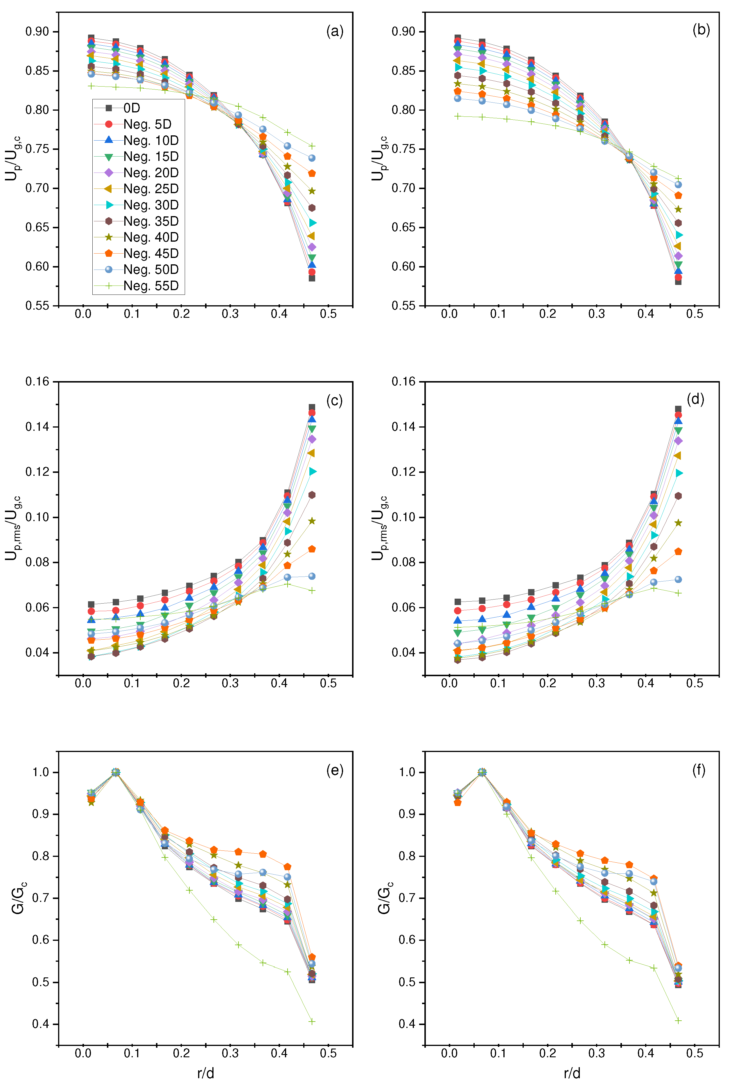
It was realized that most of the flow development occurred in the first 40 nozzle diameters, where the last 20 D experienced very minute changes in all parameters (Figure 2). The inside of the nozzle for the Lau and Nathan (Lau3, Table 1 and Table 4) test case was also examined. It was realized that full development occurred in about the first 30 nozzle diameters with only minute differences observed in the last 10 nozzle diameters; see Figure 3.

4.2. Hardalupas et al. [5] Results

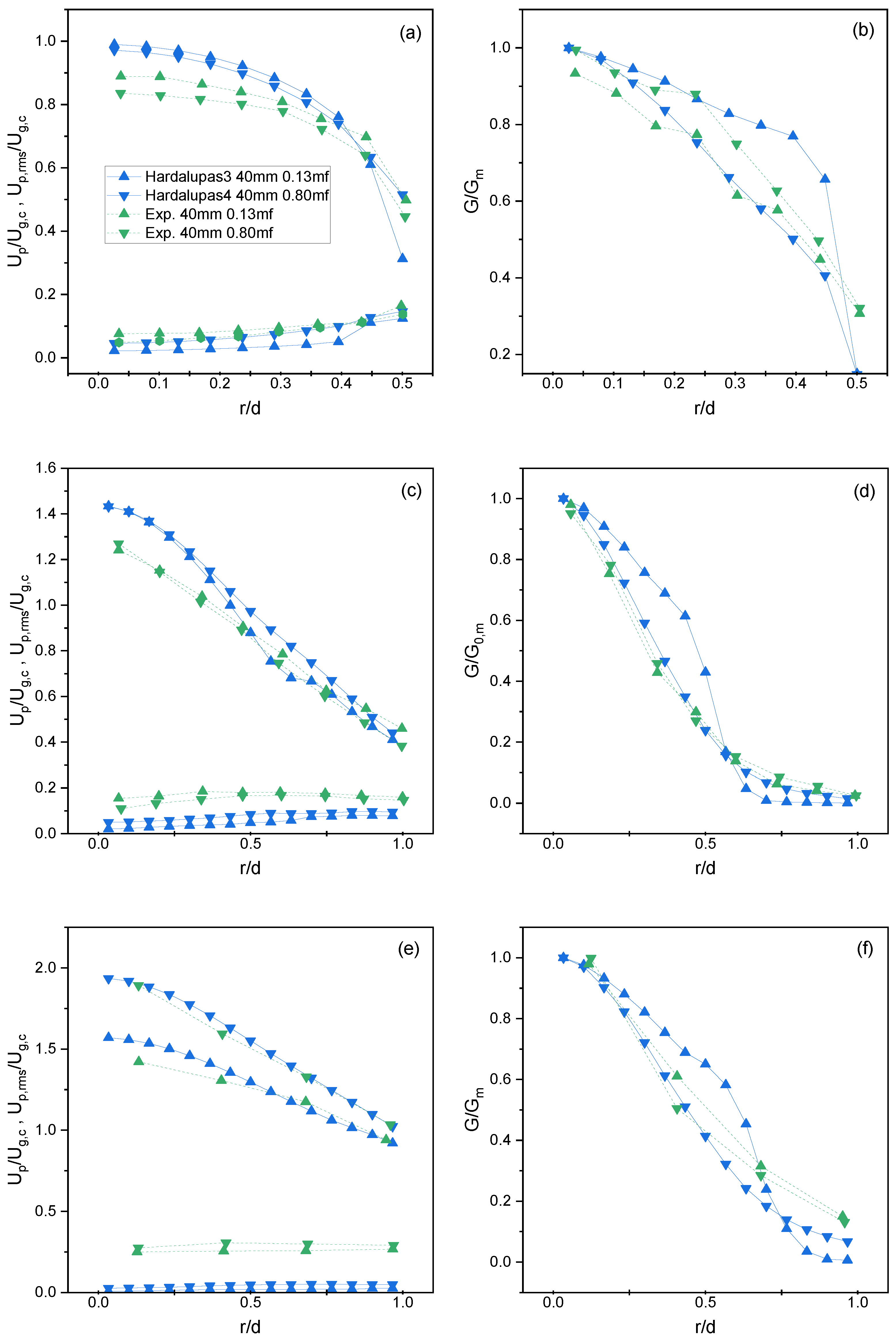
It was realized that the results at the nozzle exit for all the test cases of Hardalupas et al. [5] provided a similar trend for the mean and root-mean-squared velocity near the central regions of the jet stream. Still, towards the outer regions near the nozzle wall, it was observed that the particles moved more towards a laminar shape profile rather than a more-turbulent shape, as demonstrated by the experiments (Figure 4a and Figure 5a). This was believed to be caused by the interpolation method used for velocity in particle–fluid interactions.
To achieve effective momentum coupling, we required a cell size with a minimum length side of at least 1.86 -times the particle diameter for these types of flow problems [20]. To model the boundary layer at the wall of a CFD simulation, we either needed to fully integrate into the wall or use an algebraic function. To fully integrate into the wall, we required an extremely fine mesh with, at the very least, 8–10 cells located below y + = 11.5 [27]. Achieving this, while also achieving effective momentum coupling, would require extremely small particles, far smaller than those used in many cases, including the experimental studies considered in this current work. Therefore, a wall approach near the wall was used in this current work to accurately model the strong viscous effects on the fluid velocity while achieving effective momentum coupling. That said, there was not a perfect solution here because there was also a concern with the fluid velocity and void fraction interpolation when calculating the drag particle–fluid coupling force. A wall function was used in this current work to model the fluid boundary layer in the larger cell. Still, for interpolation, that same wall function was not used for particle coupling parameter interpolation, but instead, a linear interpolation method.
In CFD-DEM, the interpolation method used is a linear cell point method. This method breaks each face into triangles to define tetrahedra and the cell center point; then, it cycles through the tetrahedra to determine where the point or particle cell point center is located. An inverse distance linear interpolation was then used from known velocity points of the cell centers. This produces a different distribution of coupling velocities than is modeled by our wall function. Optimally, we would want to use an interpolation method that follows the wall function. This would involve developing a tracking algorithm that allows the use of a custom interpolation scheme when in the near-wall cell, but difficulties would arise that may increase the computational expense, which would have to be addressed.
Although there were discrepancies at the nozzle exit, it was observed that, further in the flowfield, there were very similar trends between the numerical and experimental results for the lower (0.23) and higher (0.86) mass fractions, respectively.
In general, for the 80 μ m particle simulations (Hardalupas1 and Hardalupas2), discrepancies were observed at the nozzle exit associated with the interpolation method for both mean (rms) velocities and particle number fluxes (Figure 4a and Table 5). As previously outlined, this can be attributed to the issues with the interpolation method near the wall. That being said, relative accuracy was achieved for the velocities where the general change in the results between the two mass fractions was similar to that of the experiments. At location 10 D , similar slopes were achieved between all numerical and experimental results. The numerical results showed a slight decrease in slope relative to the experimental results near the outer regions of the jet. At 20 D , higher mean velocities were observed for the numerical results with root-mean-squared velocities closely following and a smaller spread with the particle number fluxes. It was concluded that, with 80 μ m particles, up to 10 D should see viable results for the case of the optimization of an industrial unit, but anything further downstream would need more analysis. Work needs to be performed for pipe flows with wall functions in CFD-DEM to solve the interpolation issues, but it was observed that the particles “correct” themselves after they exit the nozzle. This could be attributed to having relatively low Stokes numbers, and therefore, the particles closely followed the highly accurate and validated fluid flow, where wall effects were not present.
For the 40 μ m particles, the same errors at the nozzle exit were observed because of interpolation for all fields, but with the same relative accuracy or change in trends between the two mass fluxes (Figure 5a,b). An interesting note for the nozzle exit is that, with smaller mass loading (Hardalupas3), a particle number flux with a flatter profile than that of the larger mass loading (Hardalupas4) was observed. It was postulated that, if mass loading continued to increase, a more-triangular profile for particle number flux would be achieved. Further downstream, similar slopes in the results for the mean velocity and particle number flux were observed, but a significantly lower root-mean-squared velocity for the numerical results. It is curious to note that these smaller particle trends lined up quite well up to 20 D , but with the larger particles results can only be trusted up to 10 D . This was further reinforced by the root-mean-squared error values shown in Table 5. It can be concluded that, as the Stokes number increased, where the particles tended to “go their own path”, the numerical results started deviating from the experimental results.

4.3. Lau and Nathan Single-Phase Results

The single-phase results for the test cases of Hardalupas et al. [5] were validated in our previous work [27], but the results of Lau and Nathan [11] were not. Therefore, three different simulation setups were used to determine that the single-phase results were accurate before adding the particulate phase. If this was not performed, then there was a risk of obtaining a model that may have the perfect combination of parameters for the two-phase flow, but not necessarily because each of the phases separately is accurate. This would make it difficult to conclude with any confidence that this model can be generally applied to other similar flows and accurately represents the physics.
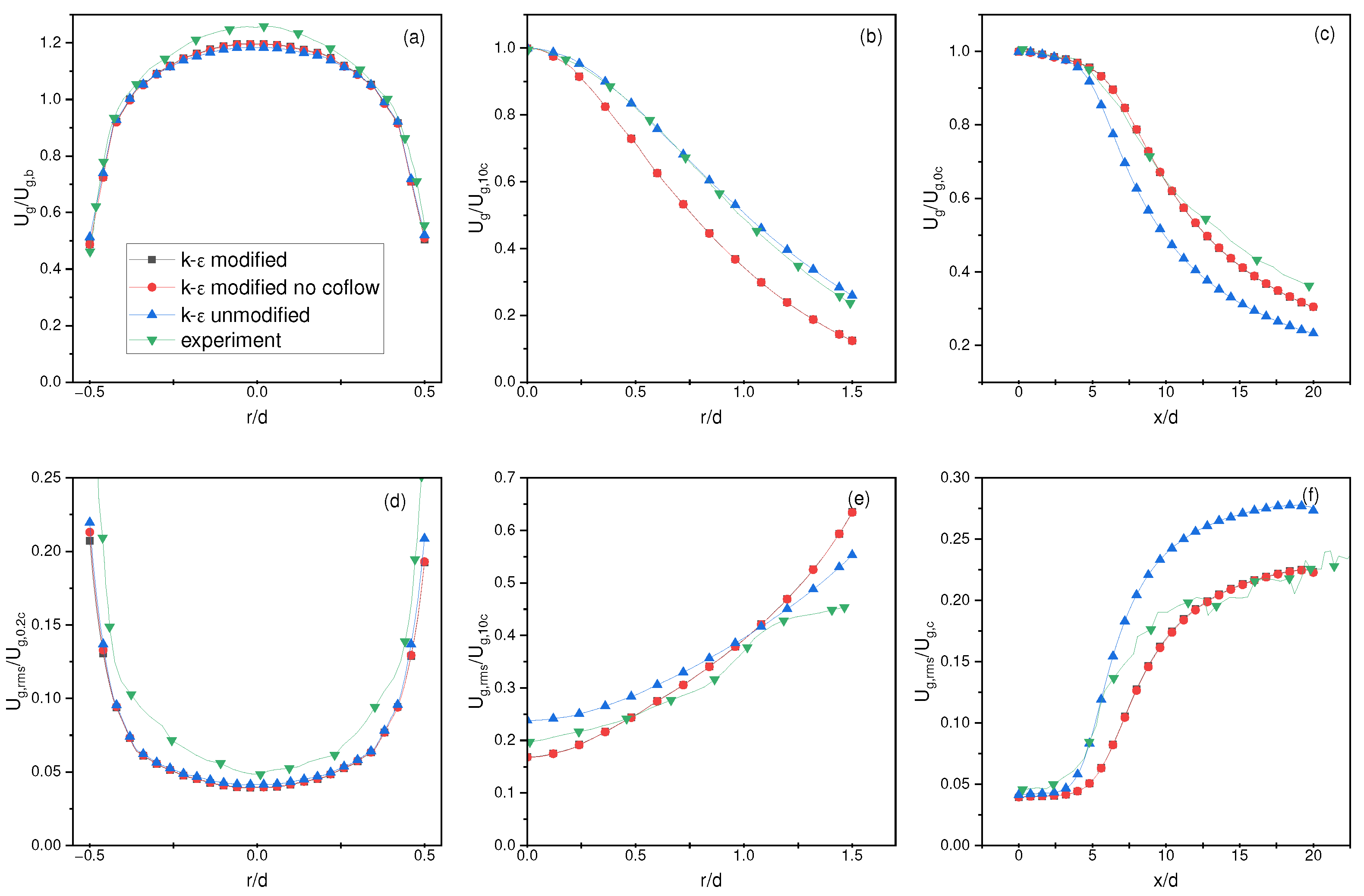
All cases started with the Lau3 test case (48 m/s), but without the inclusion of particles. The default Launder and Spalding [26] k- ε was used for one case. For the second case, a change of the empirical coefficients was made to the turbulence model by C ε 1 = 1.52 and C ε 2 = 1.90 . This modification was researched and validated extensively in our previous work [27]. The third simulation used the modified k- ε turbulence model, but without the use of co-flow. This was to test the effect that co-flow has on these types of numerical simulations.
There was very little difference between all simulations at the nozzle exit for both the mean and root-mean-squared velocities, as shown in Figure 6a,d. At location 10 D , the unmodified k- ε turbulence model produced spreading that more closely followed the experiment for mean velocity, but the modified k- ε produced a drop in axial velocity that more closely matched the experiment. Therefore, it is up to the researcher to weigh the pros and cons of using the modified k- ε , whether it is important for accurate spreading or accurate axial drop in mean velocities. That being said, in the current authors’ previous work, it was found that both spreading rates and the axial drop in the mean velocity were both improved with the slight modification of the empirical coefficients [27] for the two different sets of data provided by Bogusławski and Popiel [28] and Hardalupas et al. [5]. For the root-mean-squared velocities, the modified k- ε produced spreading rates that more closely matched the experiments at all sampling locations. There was no appreciable difference in all sampling locations in adding a co-flow to the simulations. Considering all this, it was decided to use the modified k- ε with a co-flow for all subsequent simulations for the test cases of Lau and Nathan [11].

4.4. Lau and Nathan Results

As previously noted, there will be errors at the nozzle exit associated with the interpolation method, and this also extends to the results of Lau and Nathan [11], as indicated in Figure 7a,b. A more-laminar flow profile was realized for the mean particle velocity with a higher mean velocity in the central region while decreasing rapidly towards the wall relative to the experimental results. That being said, it was observed that the overall trend when changing the Stokes number agreed with the experimental results. For example, the lowest Stokes number had the highest mean particle velocity in the central region. Conversely, the highest Stokes number had the lowest mean particle velocity for both the experiments and numerical simulations (Figure 7a). At the location 10 D , we observed a slightly steeper slope for the mean particle velocities and a slightly higher root-mean-squared velocity with the same slope. It is interesting to note that mean particle velocity changed at 10 D depending on the Stokes number. In contrast, in the experiments, the normalized mean particle velocity minimally changed between the Stokes numbers. This could be attributed to the errors at the nozzle exit, but this is difficult to postulate with confidence because we did not experience this behavior with the test cases of Hardalupas et al. [5]. It was also observed that, with increasing Stokes number, the associated Root-Mean-Squared Error (RMSE) at 0 D did not change significantly, but at 10 D , there was an obvious decrease in the error (Table 6).

4.5. Coarse-Graining Results

Some DEM simulations use a large number of particles, upwards of six-million. This would require a significant amount of compute cores to track and calculate all collisions between particles. Furthermore, developing codes to have the ability to scale to a very large amount of compute cores can be difficult because of the issues associated with the slowed communication between compute nodes. To circumvent this, many researchers have turned to coarse-graining methods. The essence of coarse-graining is that multiple particles are represented as a single grain, and then, the grain is tracked through time. This significantly decreases the number of trajectories tracked throughout the system and, depending on the type of coarse-graining model, can reduce the number of tracking points by n g = n p n p f c g 3 f c g 3 . We can see that, with a coarse-graining factor of 2, f c g = 2 , the example of 6-million particles reduced down to 750-thousand particles. This reduced the overall computational cost significantly. Furthermore, additional computational savings can be realized by increasing the integration time step, and the duration of the soft sphere collisions will generally be smaller by several orders of magnitude [39].
As previously mentioned in Section 2.4, the type of coarse-graining used for this analysis was first proposed by Radl et al. [40] and further expanded to include the Hertz nonlinear contact model by Nasato et al. [41]. Radl et al. [40] concluded that the major hurdle in using a coarse-graining approach is to correctly compute the collision rate and inter-parcel or inter-grain stress, with there being no easy way to scale the interaction parameters in an inertial flow regime [40]. This conclusion is significant because it will be difficult to relate this current work’s collision frequencies, forces, and stresses from an unscaled system (no coarse-graining) to a scaled (coarse-grained) one. That being said, if the overall trends are followed, we may find the usefulness of coarse-graining in an industrial application.
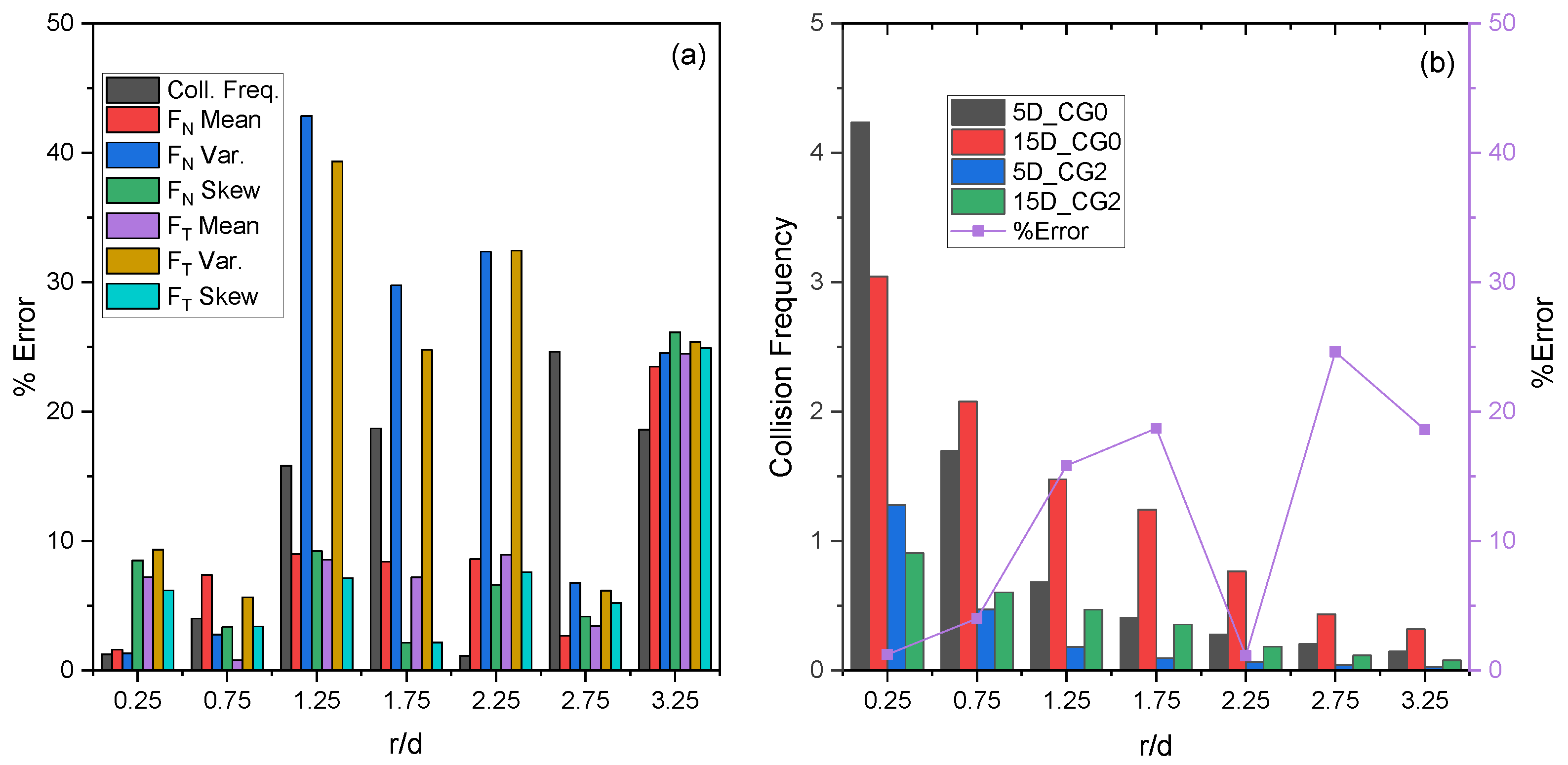
To optimize an industrial-scale unit, a statistical analysis needs to be performed on the parameters, including the collision frequencies and forces acting on particles. Therefore, at first glance, it would seem that coarse-graining should not be used in this type of setting because of the disparity between inter-grain stresses from the unscaled to scaled system. That being said, the goal of numerical simulations, and any experimental study for that matter, is to find the optimum setup through an analysis of the changes in the geometric and operating parameters. Since this is the ultimate practical goal, and it may not be necessary to obtain the exact answers of the physical space; we can, for example, compare two different geometries of an unscaled system to a scaled system using those same geometries.
To investigate the accuracy of coarse-graining, two sets of simulations with the same operating parameters as the Hardalupas1 case were performed. The first set of simulations was unscaled, while the second set was scaled. In each set, a plate was inserted at two different axial locations: 5 D and 15 D relative to the nozzle exit, resulting in four simulations in total. The collision frequencies and force statistics applied to the particles when they hit the plate for both the 5 D and 15 D cases were then output. The ratio of the results obtained from the 5 D and 15 D simulations was calculated and compared to the ratios between the scaled and unscaled systems to determine the accuracy of coarse-graining. We then analyzed the collision frequencies and mean/variances of the normal/tangential forces for all collisions (Figure 8a) and also analyzed the results grouped by location with intervals of 0.5 D on the plate. These results were then used to determine whether the coarse-graining method accurately predicted the results that followed the simulation trend of an unscaled system.
The ratios we compared for collision frequencies are given by
r a t i o c f , c g 0 = C F c g 0 , 5 D C F c g 0 , 15 D , r a t i o c f , c g 2 = C F c g 2 , 5 D C F c g 2 , 15 D
where C F c g 0 , 5 D and C F c g 0 , 15 D are the collision frequencies for the unscaled DEM method for simulations with 5D and 15D plates, respectively. C F c g 2 , 5 D and C F c g 2 , 15 D are the collision frequency for the scaled system with a coarse-graining factor of two for the simulations with 5D and 15D plates, respectively. Similarly, for the force statistics, we have
r a t i o F n , C G 0 = F n , c g 0 , 5 D F n , c g 0 , 15 D , r a t i o F n , C G 0 = F n , c g 2 , 5 D F n , c g 2 , 15 D
r a t i o F t , C G 0 = F t , c g 0 , 5 D F t , c g 0 , 15 D , r a t i o F t , C G 0 = F t , c g 2 , 5 D F t , c g 2 , 15 D
The collision frequencies and force statistics were then output for all collisions (Figure 8a) and concentric regions (Figure 8b), and the ratios and associated errors were calculated, as shown in Table 7.
It should be noted, for completeness, that the percent error was calculated from the traditional formula, given by
% E r r o r = 100 · r a t i o c g 0 r a t i o c g 2 r a t i o c g 0
When analyzing all the collisions acting on the plate, it was realized that there was an error of less than 4 % for all parameters, as indicated by Table 7. These results demonstrated the accuracy in comparing the ratios of scaled to unscaled systems when analyzing all collisions on the plate.
To further analyze the trends of particle collisions with the plate, the collisions were independently considered within specific concentric regions on the plate, as shown in Figure 8b, and the same analysis of the collision frequency and force statistics was performed.
In Figure 9, the relative errors are plotted between the scaled and unscaled system ratios for each region. A slightly different conclusion than when analyzing all collisions can be realized. The majority of the mean values had an error less than 10 % with the only region above being at r r d d = 3.25 with an error of just above 20 % . The highest errors in the force statistics were the variance errors, which were in line with the collision frequency errors; most errors were observed in regions where the collision frequency was low. To investigate this further, Figure 9b shows individual collision frequencies for both unscaled and scaled systems at 5 D and 15 D plate positions with the corresponding collision frequency ratio relative errors. It was realized that the collision frequency was high near the center region with a much lower percentage error. Conversely, the collision frequency was lowest in the outer regions with a relatively high percentage error. Considering all this, along with the very low error of less than 4 % for all collisions, it can be concluded that we achieved a relative accuracy that provided significant results for the practical application of an industrial flow problem.
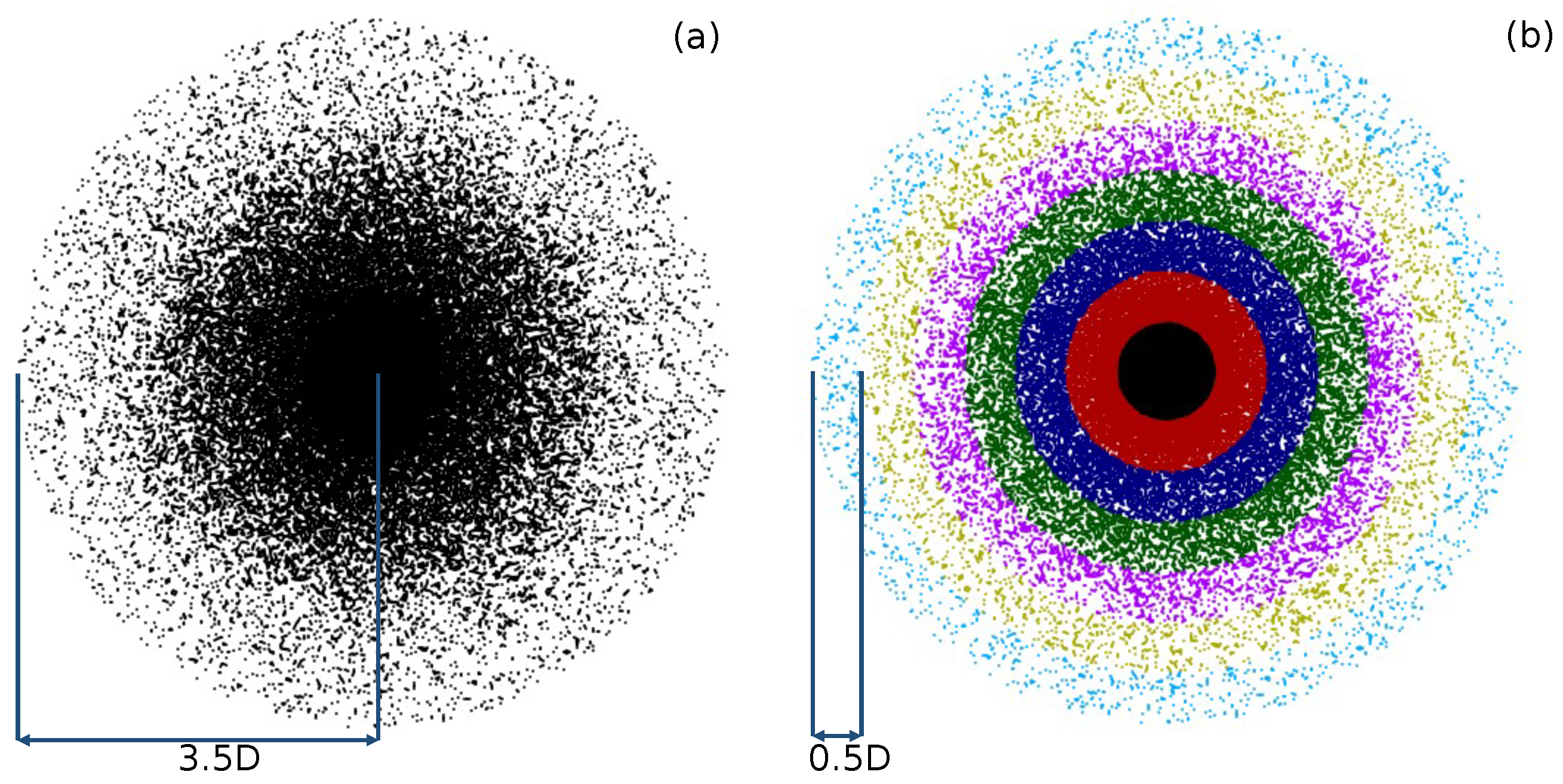
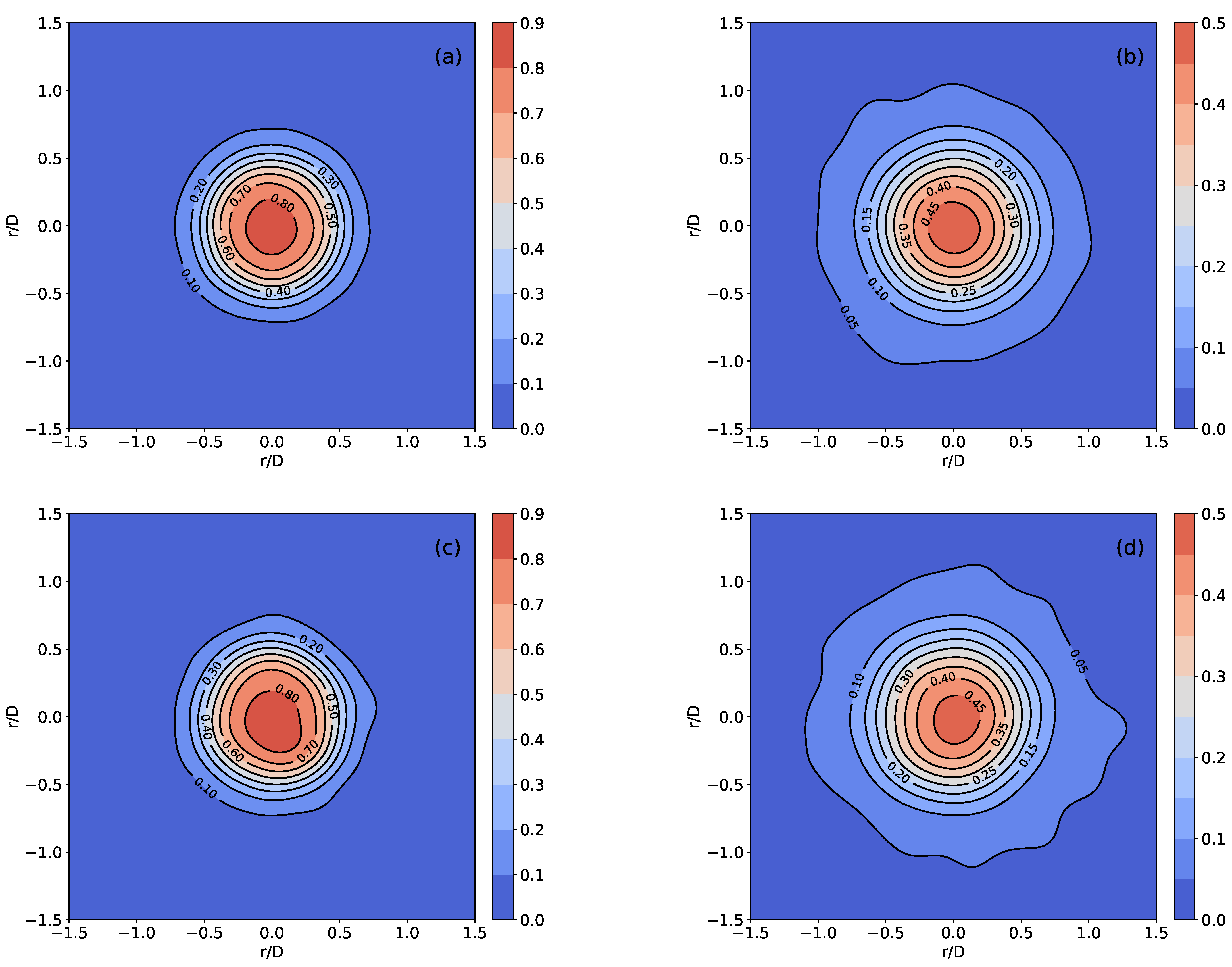
A Kernel Density Estimate plot (KDE) was then used to visualize the distribution of the collisions on the plate (Figure 10). This plot uses a Gaussian smoothing algorithm to estimate the probability density function. This allowed the visualization of the distribution of the particle impacts across the plate. It was realized that the probability of particle collisions between C G = 0 and C G = 2 was very comparable with the largest difference towards the outer regions, as demonstrated when comparing at location 15 D (Figure 10b,d). This reassuringly confirmed the use of coarse-graining for an industrial flow optimization problem.
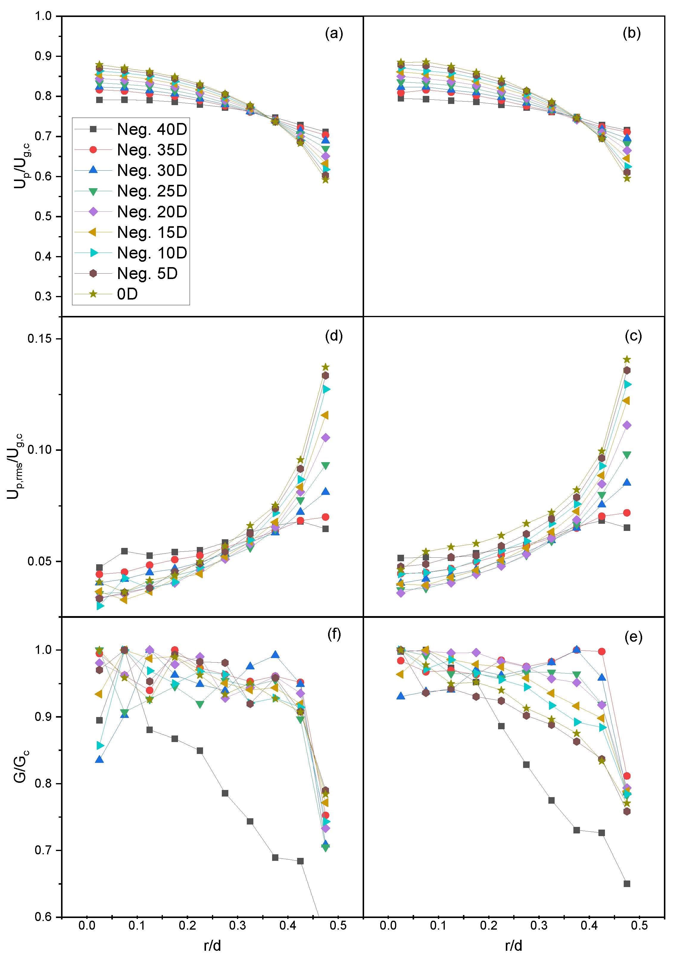
Of special interest is comparing the flow profiles both inside of the nozzle and outside of the jet. This could be beneficial in future simulations because, if flow development occurs sooner for coarse-graining, that would further reduce the computational cost by allowing a shorter nozzle.
Very little difference in the length of the full development for the particles (Figure 11) in all parameters was observed. Furthermore, it was realized that there was also very little difference between the scaled and unscaled systems in the jet stream for all fields, with the highest error being observed for the root-mean-squared velocity (Figure 12).
If the desire is to optimize an industrial unit, then the goal is to pinpoint a design that performs better than another. Therefore, from a practical standpoint, if relatively accurate answers are achieved that follow the same trends as the changes in the design of a physical system, then the goal can be reached from purely numerical simulations alone. With that in mind, coarse-graining is deemed a very useful tool in the optimization of an industrial unit for high-speed jet flows because of the significant reduction in the simulation cost. That being said, these results and conclusions should not be realized for other types of systems, in particular systems with a large amount of particle–particle collisions in a semi-quasi steady state inertial system that significantly dictates the bulk flow behavior. It is worth acknowledging that the authors express a high level of confidence in their ability to employ coarse-graining techniques when dealing with Reynolds and Stokes numbers that fall within the range of those tested. However, it is imperative to conduct additional testing for values that lie outside of this range to ensure the validity of the results.

5. Conclusions

This paper performed fully coupled CFD-DEM simulations and validated them against two different experimental studies, namely Hardalupas et al. [5] and Lau and Nathan [11]. The coupling parameters, models, and operating conditions were all considered. However, issues were encountered with the interpolation method used in the fully coupled simulations, which produced a more laminar profile shape for the particles at the nozzle exit. Future work can investigate this issue further.
For the test cases of Hardalupas et al. [5], a Stokes number of 50 can be trusted up to 10 D from the nozzle exit and a Stokes number of 10.27 can be trusted up to 20 D if only the mean and particle number fluxes are desired. The modified k-epsilon models were consistent with the single-phase results of Lau and Nathan [11], providing further validation of the previous work [27]. For the test cases of Lau and Nathan [11] at 10 D , there was a slightly steeper slope for the mean particle velocity with a higher root-mean-squared velocity. Overall, it was concluded that the CFD-DEM’s accuracy generally increased with increasing Stokes number up to 50, based on both studies.
Finally, it is noted that coarse-graining is a useful method for practical applications such as the optimization of industrial-scale units, where relative results between designs are desired. However, if the goal is to measure the total energy dissipation of a single experiment, coarse-graining falls short.

Author Contributions

Conceptualization, D.S.W. and S.M.; methodology, D.S.W. and S.M.; software, D.S.W.; validation, D.S.W.; formal analysis, D.S.W. and S.M.; investigation, D.S.W. and S.M.; resources, S.M.; data curation, D.S.W.; writing—original draft preparation, D.S.W.; writing—review and editing S.M. and D.S.W.; visualization, D.S.W.; supervision, S.M.; project administration, S.M.; funding acquisition, S.M. All authors have read and agreed to the published version of the manuscript.

Funding

The research was supported and funded by the MITACS Accelerate program and Disa TechnologiesTM (Contract No. IT23227). We gratefully acknowledge the computing support of Compute Canada via their WestGrid program and the ARC group at the University of British Columbia for providing the access to the Sockeye cluster.

Data Availability Statement

The cases, models, and data solutions can be made available by contacting the corresponding author.

Conflicts of Interest

The funders had no role in the design of the study; in the collection, analyses, or interpretation of the data; in the writing of the manuscript; nor in the decision to publish the results.

Abbreviations

The following abbreviations are used in this manuscript:
ε f liquid volume fraction, V f V g V p V p
V f volume of fluid inside of a cell
V c volume of the cell
V s particle or solid volume in the cell
ρ f density of the fluid
ρ p density of the particle
u f velocity of the liquid
u s average solid velocity inside of the cell
u p particle velocity
s w i t c h variable to change between Model A (Set II) and Model B (Set I) of the CFD-DEM formulation
ppressure
τ liquid phase stress tensor
K s l implicit momentum coupling term
fexplicit force term
F ¯ d summation of all forces inside of a cell
kfluid turbulent kinetic energy
ε fluid turbulent dissipation
ν fluid viscosity
ν t fluid turbulent viscosity
σ k k- ε constant
σ ε k- ε constant
C ε 1 k- ε constant
C ε 2 k- ε constant
S i j deviatoric part of the fluid stress tensor
δ i j Kronecker delta
m p particle mass
ggravity vector
f p pressure force
f · τ viscous force
f l lift force acting on the particle
f p p particle–particle interaction force
f p w particle–wall interaction force
f d r a g drag force
I p moment of inertia of the particle
ω p rotational velocity of the particle
T p torque acting on the particle
F c n normal contact force
F c t tangential contact force
k n normal stiffness coefficient
γ n normal damping coefficient
δ n normal overlap distance
v r n normal relative velocity
k t tangential stiffness coefficient
γ t tangential damping coefficient
δ t tangential overlap distance
v r t tangential relative velocity
β p used for the calculation of drag to further simplify the equation
u r relative velocity between the fluid and the solid, u f u s
C d the coefficient of drag
d g diameter of the grain
f c g coarse-graining factor
η f shape factor
Re p particle Reynolds number
ϕ p particle shape factor
ν f fluid viscosity
E * equivalent Young’s modulus
R * equivalent particle radius
R 1 , R 2 particle radius on collision
E 1 , E 2 particle Young’s modulus for collisions
ν 1 , ν 2 Poisson’s ratio for collisions
R g grain (parcel) radius
R p particle radius
C G 0 unscaled (no coarse-graining) system
C G 2 coarse-graining factor of 2
y + non-dimensional wall distance
u + non-dimensional velocity defined as the near-wall velocity divided
by the shear velocity
C F c g 0 , 5 D collision frequency statistic for unscaled system using 5 D plate
C F c g 0 , 15 D collision frequency statistic for unscaled system using 15 D plate
C F c g 2 , 5 D collision frequency statistic for scaled system using 5 D plate
C F c g 2 , 15 D collision frequency statistic for scaled system using 15 D plate
F n , t , c g 0 , 5 D normal or tangential force statistic for unscaled system using 5 D plate
F n , t , c g 0 , 15 D normal or tangential force statistic for unscaled system using 15 D plate
F n , t , c g 2 , 5 D normal or tangential force statistic for scaled system using 5 D plate
F n , t , c g 2 , 15 D normal or tangential force statistic for scaled system using 15 D plate

Appendix A

Dimensional analysis was used for the stiffness and damping coefficients to scale from the particles to the grains. The normal and tangential stiffness coefficients in the Hertz model are provided in the work of Di Renzo and Di Maio [36,37] and given, respectively, by
k n , p = 4 3 E * R p * δ n , p
k t , p = 8 G * R p * δ n , p
1 / E * = 1 ν 1 2 / E 1 + 1 ν 2 2 / E 2 R * = 1 / R 1 + 1 / R 2 1 G * = 2 2 v 1 1 v 2 2 E 1 + 2 2 v 2 1 + v 2 E 2
where E * is the equivalent Young’s modulus, R * is an equivalent radius, δ n is the normal overlap, G * is an equivalent shear modulus, ν is Poisson’s ratio, E is Young’s modulus, and R is the particle radius. Scaling particle radius by the factor f c g , we obtain
R g = f c g R p
R g * = f c g R p * , δ n , g = f c g δ n , p
Plugging Equation (A5) into Equations (A1) and (A2), we obtain the scaled stiffness coefficients, given by
k n , g = 4 3 E * R g * δ n , g = f c g 4 3 E * R p * δ n , p = f c g k n , p
k t , g = 8 G * R g * δ n , g = f c g 8 G * R p * δ n , p = f c g k t , p
As shown by Equations (A6) and (A7), the stiffness coefficients are merely scaled by f c g . The damping coefficients γ n , p , γ t , p for the nonlinear Hertz–Mindlin model are given in Hu et al. [57] by
γ n , p = 2 5 6 β S n , p m p * 0
γ t , p = 2 5 6 β S t , p m p * 0
S n , p = 2 E * R p * δ n , p
S t , p = 8 G * R p * δ n , p
1 1 m p * = 1 1 m 1 , p m 1 , p m p * = 1 1 m 1 , p m 1 , p + 1 1 m 2 , p m 2 , p
β = ln e n ln 2 e n + π 2
Plugging Equation (A5) into Equations (A10) and (A11), we demonstrate that S n , p and S t , p are also scaled by f c g :
S n , g = 2 E * R g * δ n , g = f c g 2 E * R p * δ n , p = f c g S n , p
S t , g = 8 G * R g * δ n , g = f c g 8 G * R p * δ n , p = f c g S t , p
To then calculate the scaling for the damping coefficient, we first needed to determine the mass. We know that density is constant from the particles to the grains, so to obtain the mass, we multiplied the density by the volume of the particle.
m p = ρ p 4 3 π R p 3
Plugging Equation (A5) into (A16), we obtain the grain mass by
m g = ρ p 4 3 π R g 3 = ρ p 4 3 π f c g 3 R p 3 = f c g 3 m p
Given Equation (A12), we can then infer that the equivalent mass scales by
m g * = f c g 3 m p *
We can now calculate the scaled damping coefficients in the normal and tangential directions by plugging Equations (A14), (A15), and (A18) into Equations (A8) and (A9) and show that the damping coefficient is scaled by f c g 2 .
γ n , g = 2 5 6 β S n , g m g * = 2 5 6 β f c g 4 S n , p m p * = f c g 2 γ n , p
γ t , g = 2 5 6 β S t , g m g * = 2 5 6 β f c g 4 S t , p m p * = f c g 2 γ t , p
Based on the non-dimensional analysis work of Radl et al. [40] and Nasato et al. [41], a linear spring–dashpot model does not have a nonlinear function of particle radius, but only constant values for the stiffness and damping coefficients. We observed that, after scaling the grains’ radius, there was no need to additionally scale both the stiffness and damping parameters because they already scaled with f c g and f c g 2 , respectively. Therefore, merely the particle radius was scaled by the coarse-graining factor.

References

  1. Coates, E.; Lee, J. High Slurry Density Hydraulic Disassociation System. U.S. Patent 9815066, 4 January 2022. [Google Scholar]
  2. Coates, J.A.; Seriven, D.H.; Coates, C.; Coates, E. Methods for Processing Heterogeneous Materials. U.S. Patent 11213829, 4 January 2022. [Google Scholar]
  3. Coates, J.A.; Seriven, D.H.; Coates, C.; Coates, E. Devices, Systems, and Methods for Processing Heterogeneous Materials. U.S. Patent 8646705, 11 February 2014. [Google Scholar]
  4. Coates, J.A.; Seriven, D.H.; Coates, C.; Coates, E. Devices, Systems, and Methods for Processing Heterogeneous Materials. U.S. Patent 9914132, 13 March 2018. [Google Scholar]
  5. Hardalupas, Y.; Taylor, A.; Whitelaw, J. Velocity and particle-flux characteristics of turbulent particle-laden jets. Proc. R. Soc. London A Math. Phys. Sci. 1989, 426, 31–78. [Google Scholar] [CrossRef]
  6. Levy, Y.; Lockwood, F.C. Velocity measurements in a particle laden turbulent free jet. Combust. Flame 1981, 40, 333–339. [Google Scholar] [CrossRef]
  7. McComb, W.; Salih, S. Measurement of normalised radial concentration profiles in a turbulent aerosol jet, using a laser-doppler anemometer. J. Aerosol Sci. 1977, 8, 171–181. [Google Scholar] [CrossRef]
  8. Modarress, D.; Wuerer, J.; Elghobashi, S. An Experimental Study of a Turbulence Round Two-Phase Jet. Chem. Eng. Commun. 1984, 28, 341–354. [Google Scholar] [CrossRef]
  9. Popper, J.; Abuaf, N.; Hetsroni, G. Velocity measurements in a two-phase turbulent jet. Int. J. Multiph. Flow 1974, 1, 715–726. [Google Scholar] [CrossRef]
  10. Shuen, J.S. A Theoretical and Experimental Investigation of Dilute Particle-Laden Turbulent Gas Jets (two-Phase Flow). Ph.D. Thesis, The Pennsylvania State University, State College, PA, USA, 1984. [Google Scholar]
  11. Lau, T.C.W.; Nathan, G.J. The effect of Stokes number on particle velocity and concentration distributions in a well-characterised, turbulent, co-flowing two-phase jet. J. Fluid Mech. 2016, 809, 72–110. [Google Scholar] [CrossRef] [Green Version]
  12. Fernandes, C.; Semyonov, D.; Ferrás, L.L.; Nóbrega, J.M. Validation of the CFD-DPM solver DPMFoam in OpenFOAM® through analytical, numerical and experimental comparisons. Granul. Matter 2018, 20, 64. [Google Scholar] [CrossRef]
  13. Karimi, M.; Mostoufi, N.; Zarghami, R.; Sotudeh-Gharebagh, R. A new method for validation of a CFD–DEM model of gas–solid fluidized bed. Int. J. Multiph. Flow 2012, 47, 133–140. [Google Scholar] [CrossRef]
  14. Kloss, C.; Goniva, C.; Hager, A.; Amberger, S.; Pirker, S. Models, algorithms and validation for opensource DEM and CFD-DEM. Prog. Comput. Fluid Dyn. Int. J. 2012, 12, 140. [Google Scholar] [CrossRef]
  15. Mansouri, A.; Arabnejad, H.; Shirazi, S.; McLaury, B. A combined CFD/experimental methodology for erosion prediction. Wear 2015, 332–333, 1090–1097. [Google Scholar] [CrossRef]
  16. Nguyen, V.; Nguyen, Q.; Liu, Z.; Wan, S.; Lim, C.; Zhang, Y. A combined numerical–experimental study on the effect of surface evolution on the water–sand multiphase flow characteristics and the material erosion behavior. Wear 2014, 319, 96–109. [Google Scholar] [CrossRef]
  17. Pozzetti, G.; Peters, B. A numerical approach for the evaluation of particle-induced erosion in an abrasive waterjet focusing tube. Powder Technol. 2018, 333, 229–242. [Google Scholar] [CrossRef]
  18. Wang, Q.; Huang, Q.; Sun, X.; Zhang, J.; Karimi, S.; Shirazi, S.A. Large Eddy Simulation of Slurry Erosion in Submerged Impinging Jets. In Proceedings of the Computational Fluid Dynamics; Micro and Nano Fluid Dynamics, Virtual Online, 13–15 July 2020; American Society of Mechanical Engineers: New York, NY, USA, 2020; p. V003T05A040. [Google Scholar] [CrossRef]
  19. Bazdidi-Tehrani, F.; Zeinivand, H. Presumed PDF modeling of reactive two-phase flow in a three dimensional jet-stabilized model combustor. Energy Convers. Manag. 2010, 51, 225–234. [Google Scholar] [CrossRef]
  20. Weaver, D.; Miskovic, S. Analysis of Coupled CFD-DEM Simulations in Dense Particle-Laden Turbulent Jet Flow. In Proceedings of the Fluid Mechanics; Multiphase Flows, Virtual Online, 13–15 July 2020; Volume 2, p. V002T04A021. [Google Scholar] [CrossRef]
  21. Wilcox, D.C. Turbulence Modeling for CFD, 3rd ed.; Number Book, Whole in 1; DCW Industries: La Cãnada, CA, USA, 2006. [Google Scholar]
  22. Pope, S.B. An explanation of the turbulent round-jet/plane-jet anomaly. AIAA J. 1978, 16, 279–281. [Google Scholar] [CrossRef]
  23. Faghani, E.; Saemi, S.D.; Maddahian, R.; Farhanieh, B. On the effect of inflow conditions in simulation of a turbulent round jet. Arch. Appl. Mech. 2011, 81, 1439–1453. [Google Scholar] [CrossRef]
  24. Givi, P.; Ramos, J. On the calculation of heat and momentum transport in a round jet. Int. Commun. Heat Mass Transf. 1984, 11, 173–182. [Google Scholar] [CrossRef]
  25. Morgans, R.C.; Dally, B.B.; Nathan, G.J.; Lanspeary, P.V.; Fletcher, D.F. Applications of the Revised Wilcox 1998 K-Omega Turbulence Model To A Jet In Co-Flow. In Proceedings of the CFD in the Minerals and Process Industries, Melbourne, VI, Australia, 6–8 December 1999; p. 6. [Google Scholar]
  26. Launder, B.E.; Spalding, D.B. The numerical computation of turbulent flows. Comput. Methods Appl. Mech. Eng. 1974, 3, 269–289. [Google Scholar] [CrossRef]
  27. Weaver, D.S.; Mišković, S. A Study of RANS Turbulence Models in Fully Turbulent Jets: A Perspective for CFD-DEM Simulations. Fluids 2021, 6, 271. [Google Scholar] [CrossRef]
  28. Bogusławski, L.; Popiel, C.O. Flow structure of the free round turbulent jet in the initial region. J. Fluid Mech. 1979, 90, 531–539. [Google Scholar] [CrossRef]
  29. GmbH, D.C. About CFDEM(R)coupling; CFDEMresearch GmbH: Linz, Austria, 2017. [Google Scholar]
  30. Zhou, Z.Y.; Kuang, S.B.; Chu, K.W.; Yu, A.B. Discrete particle simulation of particle–fluid flow: Model formulations and their applicability. J. Fluid Mech. 2010, 661, 482–510. [Google Scholar] [CrossRef]
  31. Clarke, D.A.; Sederman, A.J.; Gladden, L.F.; Holland, D.J. Investigation of Void Fraction Schemes for Use with CFD-DEM Simulations of Fluidized Beds. Ind. Eng. Chem. Res. 2018, 57, 3002–3013. [Google Scholar] [CrossRef]
  32. Freireich, B.; Kodam, M.; Wassgren, C. An exact method for determining local solid fractions in discrete element method simulations. AIChE J. 2010, 56, 3036–3048. [Google Scholar] [CrossRef]
  33. Verlet, L. Computer “Experiments” on Classical Fluids. I. Thermodynamical Properties of Lennard-Jones Molecules. Phys. Rev. 1967, 159, 98–103. [Google Scholar] [CrossRef] [Green Version]
  34. Otsubo, M.; O’Sullivan, C.; Shire, T. Empirical assessment of the critical time increment in explicit particulate discrete element method simulations. Comput. Geotech. 2017, 86, 67–79. [Google Scholar] [CrossRef] [Green Version]
  35. Hanley, K.J.; O’Sullivan, C.; Huang, X. Particle-scale mechanics of sand crushing in compression and shearing using DEM. Soils Found. 2015, 55, 1100–1112. [Google Scholar] [CrossRef] [Green Version]
  36. Di Renzo, A.; Di Maio, F.P. Comparison of contact-force models for the simulation of collisions in DEM-based granular flow codes. Chem. Eng. Sci. 2004, 59, 525–541. [Google Scholar] [CrossRef]
  37. Di Renzo, A.; Di Maio, F.P. An improved integral non-linear model for the contact of particles in distinct element simulations. Chem. Eng. Sci. 2005, 60, 1303–1312. [Google Scholar] [CrossRef]
  38. Andrews, M.; O’Rourke, P. The multiphase particle-in-cell (MP-PIC) method for dense particulate flows. Int. J. Multiph. Flow 1996, 22, 379–402. [Google Scholar] [CrossRef]
  39. Di Renzo, A.; Napolitano, E.; Di Maio, F. Coarse-Grain DEM Modelling in Fluidized Bed Simulation: A Review. Processes 2021, 9, 279. [Google Scholar] [CrossRef]
  40. Radl, S.; Radeke, C.; Khinast, J.G.; Sundaresan, S. Parcel-Based Approach for the Simulation of Gas-Particle Flows. In Proceedings of the CFD, SINTEF/NTNU, Trondheim Norway, 3–4 October 2011; p. 11. [Google Scholar]
  41. Nasato, D.S.; Goniva, C.; Pirker, S.; Kloss, C. Coarse Graining for Large-scale DEM Simulations of Particle Flow–An Investigation on Contact and Cohesion Models. Procedia Eng. 2015, 102, 1484–1490. [Google Scholar] [CrossRef] [Green Version]
  42. Ishigaki, M.; Abe, S.; Sibamoto, Y.; Yonomoto, T. Influence of mesh non-orthogonality on numerical simulation of buoyant jet flows. Nucl. Eng. Des. 2017, 314, 326–337. [Google Scholar] [CrossRef]
  43. Weller, H.G.; Tabor, G.; Jasak, H.; Fureby, C. A tensorial approach to computational continuum mechanics using object-oriented techniques. Comput. Phys. 1998, 12, 620. [Google Scholar] [CrossRef]
  44. Jaroslav, S. Contribution to investigation of turbulent mean-flow velocity profile in pipe of circular cross-section. In Proceedings of the 35th Meeting of Departments of Fluid Mechanics and Thermomechanics, Samorín–Cilistov, Slovak Republic, 20–23 June 2016; p. 020010. [Google Scholar] [CrossRef] [Green Version]
  45. Kalitzin, G.; Medic, G.; Iaccarino, G.; Durbin, P. Near-wall behavior of RANS turbulence models and implications for wall functions. J. Comput. Phys. 2005, 204, 265–291. [Google Scholar] [CrossRef]
  46. Chen, H.; Xiao, Y.; Liu, Y.; Shi, Y. Effect of Young’s modulus on DEM results regarding transverse mixing of particles within a rotating drum. Powder Technol. 2017, 318, 507–517. [Google Scholar] [CrossRef]
  47. Lommen, S.; Schott, D.; Lodewijks, G. DEM speedup: Stiffness effects on behavior of bulk material. Particuology 2014, 12, 107–112. [Google Scholar] [CrossRef]
  48. Lorenz, A.; Tuozzolo, C.; Louge, M.Y. Measurements of impact properties of small, nearly spherical particles. Exp. Mech. 1997, 37, 292–298. [Google Scholar] [CrossRef]
  49. Sandeep, C.S.; Luo, L.; Senetakis, K. Effect of Grain Size and Surface Roughness on the Normal Coefficient of Restitution of Single Grains. Materials 2020, 13, 814. [Google Scholar] [CrossRef] [Green Version]
  50. Tang, H.; Song, R.; Dong, Y.; Song, X. Measurement of Restitution and Friction Coefficients for Granular Particles and Discrete Element Simulation for the Tests of Glass Beads. Materials 2019, 12, 3170. [Google Scholar] [CrossRef] [Green Version]
  51. Lau, T.C.; Nathan, G.J. Influence of Stokes number on the velocity and concentration distributions in particle-laden jets. J. Fluid Mech. 2014, 757, 432–457. [Google Scholar] [CrossRef] [Green Version]
  52. Ergun, S. Fluid Flow through Packed Columns. Chem. Eng. Process 1952, 48, 89–94. [Google Scholar]
  53. Wen, C.Y.; Yu, Y. Mechanics of fluidization. Chem. Eng. Prog. Symp. Ser. 1966, 62, 100–111. [Google Scholar]
  54. Zhu, H.; Zhou, Z.; Yang, R.; Yu, A. Discrete particle simulation of particulate systems: Theoretical developments. Chem. Eng. Sci. 2007, 62, 3378–3396. [Google Scholar] [CrossRef]
  55. Latzko, H. Warmubergang an einem Turbulenten. Z. Angew. Math. 1921, 1, 268–290. [Google Scholar]
  56. Mena, S.E.; Curtis, J.S. Experimental data for solid–liquid flows at intermediate and high Stokes numbers. J. Fluid Mech. 2020, 883, A24. [Google Scholar] [CrossRef]
  57. Hu, G.; Hu, Z.; Jian, B.; Liu, L.; Wan, H. On the Determination of the Damping Coefficient of Non-linear Spring-dashpot System to Model Hertz Contact for Simulation by Discrete Element Method. J. Comput. 2011, 6, 984–988. [Google Scholar] [CrossRef]
Figure 1. Domains for the test cases of Hardalupas et al. [5] and Lau and Nathan [11] with nozzle diameters of D H = 15 mm and D L N = 12.7 mm, respectively.
Fluids 08 00215 g001
Figure 2. Radial profiles for the particles’ (a,b) mean and (c,d) root-mean-squared velocity and (e,f) number flux for fully developed flow at locations 0 D and negative 5 D , 10 D , 15 D , 20 D , 25 D , 30 D , 35 D , 40 D , 45 D , 50 D , and 55 D for a mean inlet velocity of 12.8 m/s (a,c,e) and 11.94 m/s (d,b,f), respectively.
Fluids 08 00215 g002
Figure 3. Radial profiles of the particles’ (a,b) velocities (c) and flux for locations of 0 D and negative 5 D , 10 D , 15 D , 20 D , 25 D , 30 D , 35 D , and 40 D from the nozzle exit for the Lau3 simulation (48 m/s).
Fluids 08 00215 g003
Figure 4. Radial profiles for mean and root-mean-squared velocity and particle flux at 0.1D (a,b), 10D (c,d), and 20D (e,f) from the nozzle exit for the Hardalupas1 and Hardalupas2 simulations and the experimental data of Hardalupas et al. [5] (80 μ m-sized particles).
Fluids 08 00215 g004
Figure 5. Radial profiles for mean and root-mean-squared velocity and particle flux at 0.1 D (a,b), 10 D (c,d), and 20 D (e,f) from the nozzle exit for the Hardalupas3 and Hardalupas4 simulations and the experimental data of Hardalupas et al. [5] ( 40 μ m -sized particles).
Fluids 08 00215 g005
Figure 6. CFD comparison of turbulence models and experiments for (ac) mean and (df) root-mean-squared velocity at 0.2 D , 10 D , and axial locations, respectively.
Fluids 08 00215 g006
Figure 7. Radial profiles of Lau and Nathan [11] for mean and root-mean-squared velocity and particle flux at (a,b) 0.1 D and (c,d) 10 D .
Fluids 08 00215 g007
Figure 8. A snapshot in time showing particles contacting the plate: (a) all collisions on a full plate ( 3.5 D radius) and (b) collisions grouped by concentric regions with a 0.5 D width.
Fluids 08 00215 g008
Figure 9. Percent Error (a) between ratios of CG0 and CG2 and collision frequencies and (b) Percent Error for the collision frequency.
Fluids 08 00215 g009
Figure 10. A kernel density estimate plot for collision frequency on the plate in the (a) unscaled 5 D , (b) unscaled 15 D , (c) scaled 5 D , and (d) scaled 15 D simulations.
Fluids 08 00215 g010
Figure 11. Flow profiles for particles’ (a,b) mean and (c,d) root-mean-squared velocity and (e,f) number flux at locations 0 D and negative 5 D , 10 D , 15 D , 20 D , 25 D , 30 D , 35 D , and 40 D relative to the nozzle exit for CG0 and CG2, respectively.
Fluids 08 00215 g011
Figure 12. Mean and root-mean-squared particle velocity and particle number flux for locations 0 D , 2 D , 4 D , 6 D , 8 D , 10 D , 12 D , and 14 D relative to the nozzle exit.
Fluids 08 00215 g012
Table 1. Summary of particle operating and flow conditions for the selected validation cases.
Simulation NameParticle Diameter, μ mParticle Density, kg/mMass LoadingGas Exit Velocity, m/sReynolds NumberStokes Number
Hardalupas18029500.231313,00050
Hardalupas28029500.861313,00050
Hardalupas34024200.131313,00010.27
Hardalupas44024200.801313,00010.27
Lau14012000.401210,0005.6
Lau24012000.402420,00011.2
Lau34012000.404840,00022.4
Table 2. Mesh quality details.
ExperimentNumber CellsOrthogonality MaxOrthogonality AverageSkew MaxAverage y+
Hardalupas et al. [5]3,806,39721.92.90.524
Lau and Nathan [11]3,440,57825.83.10.524–76
Table 3. Summary of boundary conditions used in simulations.
LocationVelocityPressureEddy ViscosityKinetic EnergyEpsilon
WallNo SlipZero GradientSpalding Wall Func.Zero GradientEpsilon Wall Func.
Inlet u max 1 r r R R 1 1 n n Zero GradientCalculated 1.5 i u 2 C ω 3 / 4 k 3 / 2 k 3 / 2 l l
OutletEntrainment Vel.Total PressureCalculatedZero GradientZero Gradient
Initial FreestreamUniform 0Uniform 00 k = 1.5 i u 2 C ω 3 / 4 k 3 / 2 k 3 / 2 l l
Table 4. Particle initial mean and fluctuating velocities, DEM time step, and percentage of Rayleigh and Hertz critical time steps for each simulation.
Simulation NameInlet Velocity (45 D), m/sFluctuating Velocity, m/sDEM Time Step, s% Rayleigh% Hertz
Hardalupas1 11.94 1.20 , 0.45 , 0.45 10 6 5.95.3
Hardalupas2 11.94 1.20 , 0.45 , 0.45 10 6 5.95.3
Hardalupas3 11.65 1.42 , 0.45 , 0.45 5 · 10 7 6.65.7
Hardalupas4 11.65 1.42 , 0.45 , 0.45 5 · 10 7 6.65.7
Lau1 12.08 0.54 , 0.14 , 0.14 5 · 10 7 9.27.6
Lau2 22.56 0.86 , 0.24 , 0.24 2.5 · 10 7 4.64.3
Lau3 41.80 1.34 , 0.37 , 0.37 1.25 · 10 7 2.32.5
Table 5. Root-mean-squared error for the simulation data of Hardalupas et al. [5].
Simulation
Name
U p U p U g , c U g , c U p , r m s U p , r m s U g , c U g , c G G G m G m
0 . 1 D 10 D 20 D 0 . 1 D 10 D 20 D 0 . 1 D 10 D 20 D
Hardalupas10.0710.0900.1780.0230.0290.0630.2230.0950.095
Hardalupas20.0540.0360.3010.0130.0120.0500.1220.0490.116
Hardalupas30.0560.1100.0740.0510.1230.2390.1570.1410.114
Hardalupas40.0960.1290.0550.0060.0700.2470.0910.0350.130
Table 6. Root-mean-squared error for the simulation data of Lau and Nathan [11].
Simulation
Name
U p U p U g , b U g , b U p , r m s U p , r m s U p U p G G G b G b
0 . 2 D 10 D 0 . 2 D 10 D 0 . 2 D
Lau10.1570.1650.1300.0290.229
Lau20.1390.1260.1140.0400.117
Lau30.1620.0730.1090.0680.202
Table 7. Ratios of 5D and 15D collision frequencies and normal and tangential force statistics for unscaled (CG0) and scaled (CG2) systems with their relative errors.
RatioCol. Freq. F n Mean F n Var. F n Skew F t Mean F t Var. F t Skew
CG01.220.700.641.380.730.561.12
CG21.250.680.621.420.750.551.10
%Error2.393.103.783.563.811.041.23
Disclaimer/Publisher’s Note: The statements, opinions and data contained in all publications are solely those of the individual author(s) and contributor(s) and not of MDPI and/or the editor(s). MDPI and/or the editor(s) disclaim responsibility for any injury to people or property resulting from any ideas, methods, instructions or products referred to in the content.

