

An Analysis of CFD-DEM with Coarse Graining for Turbulent Particle-Laden Jet Flows


Abstract
:1. Introduction
2. Numerical Methodology
2.1. CFD
2.2. DEM
2.3. CFD-DEM Coupling
2.4. Coarse-Graining
3. Simulation Setup
3.1. Generalized CFD Setup
3.2. Generalized DEM Setup
3.3. Hardalupas et al. [5] DEM Setup
3.4. Lau and Nathan [11] DEM Setup
3.5. Coupling Setup
4. Results and Discussion
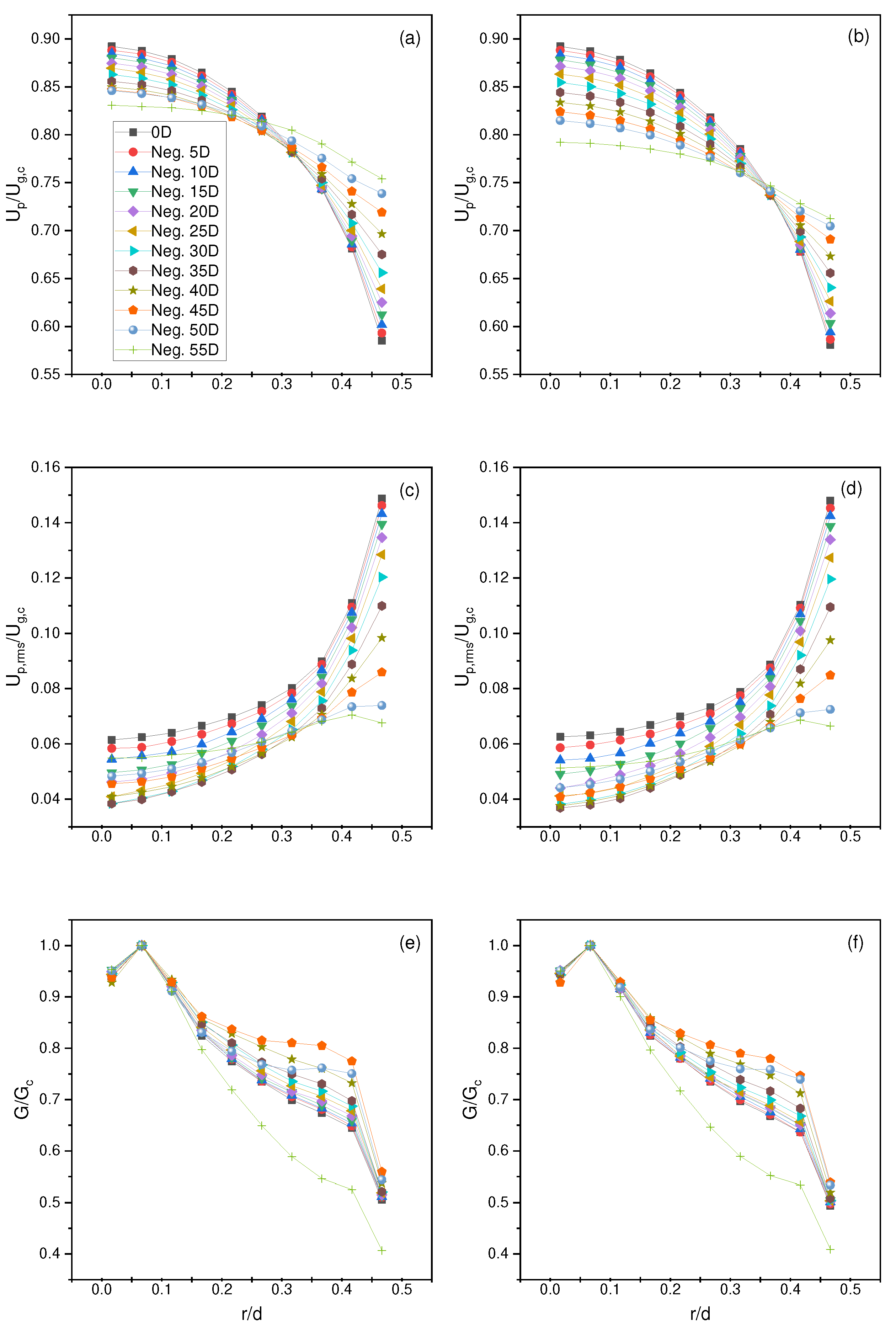
4.1. Particle Full Development
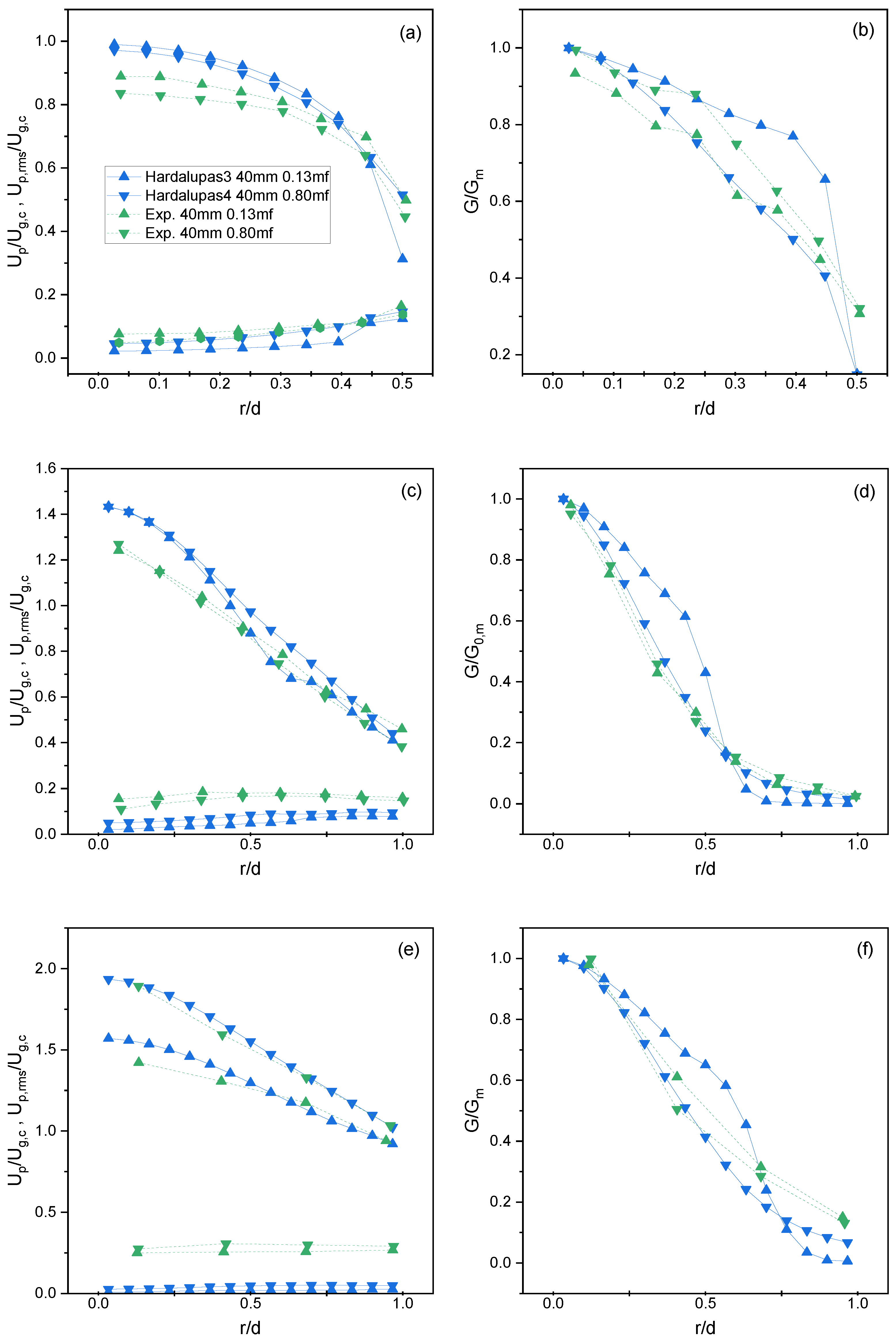
4.2. Hardalupas et al. [5] Results
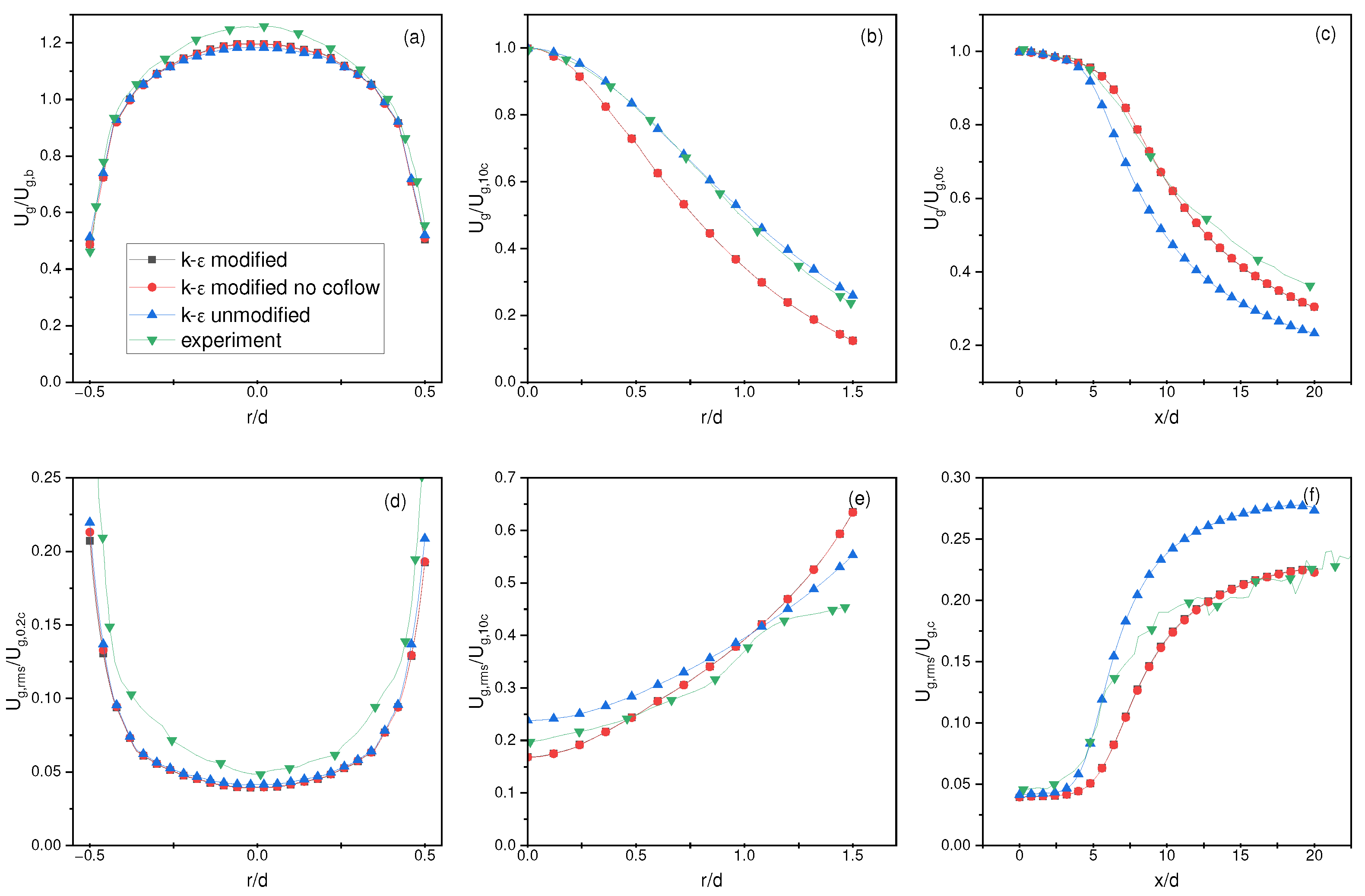
4.3. Lau and Nathan Single-Phase Results
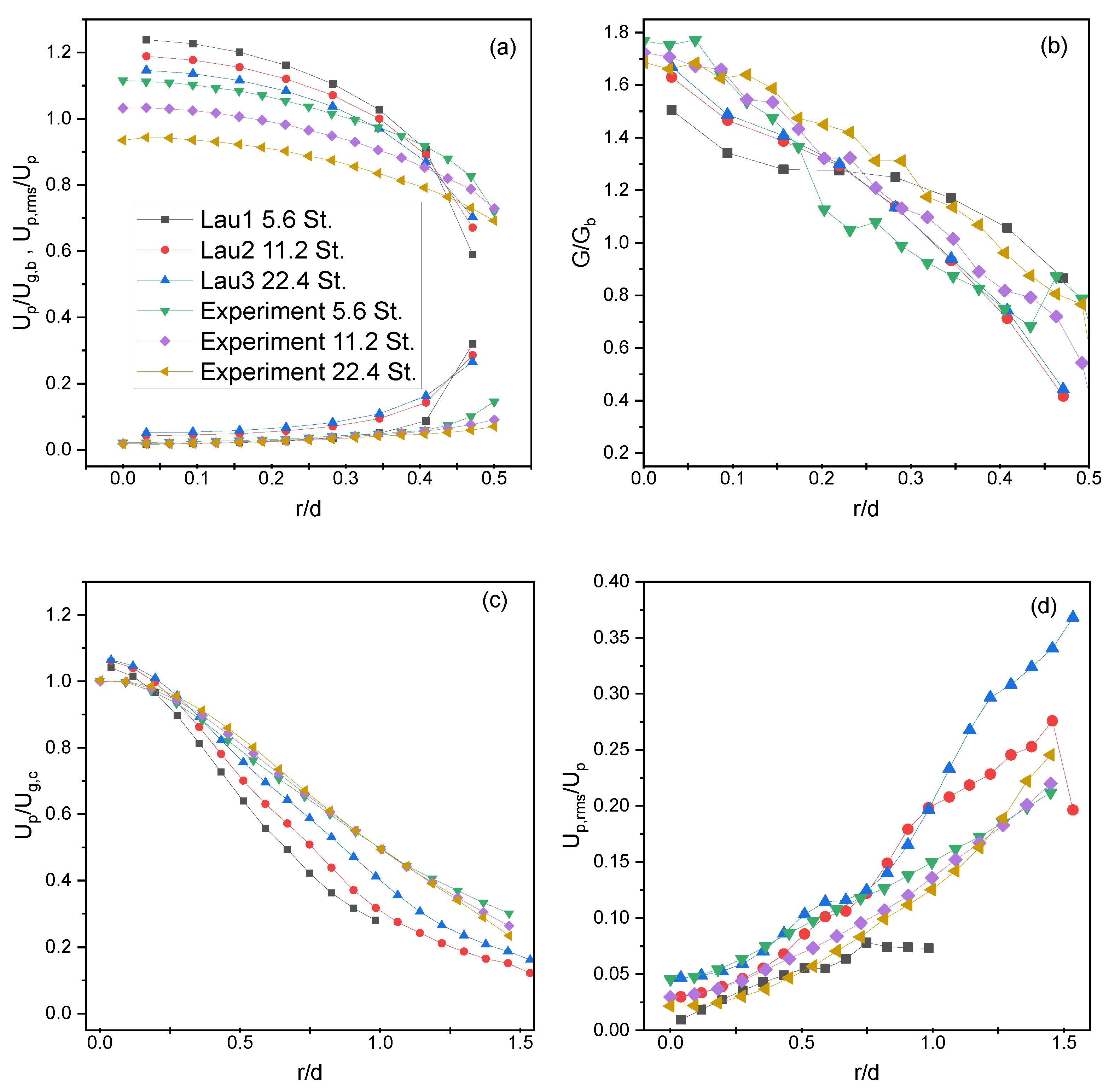
4.4. Lau and Nathan Results
4.5. Coarse-Graining Results
5. Conclusions
Author Contributions
Funding
Data Availability Statement
Conflicts of Interest
Abbreviations
| liquid volume fraction, | |
| volume of fluid inside of a cell | |
| volume of the cell | |
| particle or solid volume in the cell | |
| density of the fluid | |
| density of the particle | |
| velocity of the liquid | |
| average solid velocity inside of the cell | |
| particle velocity | |
| variable to change between Model A (Set II) and Model B (Set I) of the CFD-DEM formulation | |
| p | pressure |
| liquid phase stress tensor | |
| implicit momentum coupling term | |
| f | explicit force term |
| summation of all forces inside of a cell | |
| k | fluid turbulent kinetic energy |
| fluid turbulent dissipation | |
| fluid viscosity | |
| fluid turbulent viscosity | |
| k- constant | |
| k- constant | |
| k- constant | |
| k- constant | |
| deviatoric part of the fluid stress tensor | |
| Kronecker delta | |
| particle mass | |
| g | gravity vector |
| pressure force | |
| viscous force | |
| lift force acting on the particle | |
| particle–particle interaction force | |
| particle–wall interaction force | |
| drag force | |
| moment of inertia of the particle | |
| rotational velocity of the particle | |
| torque acting on the particle | |
| normal contact force | |
| tangential contact force | |
| normal stiffness coefficient | |
| normal damping coefficient | |
| normal overlap distance | |
| normal relative velocity | |
| tangential stiffness coefficient | |
| tangential damping coefficient | |
| tangential overlap distance | |
| tangential relative velocity | |
| used for the calculation of drag to further simplify the equation | |
| relative velocity between the fluid and the solid, | |
| the coefficient of drag | |
| diameter of the grain | |
| coarse-graining factor | |
| shape factor | |
| particle Reynolds number | |
| particle shape factor | |
| fluid viscosity | |
| equivalent Young’s modulus | |
| equivalent particle radius | |
| particle radius on collision | |
| particle Young’s modulus for collisions | |
| Poisson’s ratio for collisions | |
| grain (parcel) radius | |
| particle radius | |
| unscaled (no coarse-graining) system | |
| coarse-graining factor of 2 | |
| non-dimensional wall distance | |
| non-dimensional velocity defined as the near-wall velocity divided | |
| by the shear velocity | |
| collision frequency statistic for unscaled system using plate | |
| collision frequency statistic for unscaled system using plate | |
| collision frequency statistic for scaled system using plate | |
| collision frequency statistic for scaled system using plate | |
| normal or tangential force statistic for unscaled system using plate | |
| normal or tangential force statistic for unscaled system using plate | |
| normal or tangential force statistic for scaled system using plate | |
| normal or tangential force statistic for scaled system using plate |
Appendix A
References
- Coates, E.; Lee, J. High Slurry Density Hydraulic Disassociation System. U.S. Patent 9815066, 4 January 2022. [Google Scholar]
- Coates, J.A.; Seriven, D.H.; Coates, C.; Coates, E. Methods for Processing Heterogeneous Materials. U.S. Patent 11213829, 4 January 2022. [Google Scholar]
- Coates, J.A.; Seriven, D.H.; Coates, C.; Coates, E. Devices, Systems, and Methods for Processing Heterogeneous Materials. U.S. Patent 8646705, 11 February 2014. [Google Scholar]
- Coates, J.A.; Seriven, D.H.; Coates, C.; Coates, E. Devices, Systems, and Methods for Processing Heterogeneous Materials. U.S. Patent 9914132, 13 March 2018. [Google Scholar]
- Hardalupas, Y.; Taylor, A.; Whitelaw, J. Velocity and particle-flux characteristics of turbulent particle-laden jets. Proc. R. Soc. London A Math. Phys. Sci. 1989, 426, 31–78. [Google Scholar] [CrossRef]
- Levy, Y.; Lockwood, F.C. Velocity measurements in a particle laden turbulent free jet. Combust. Flame 1981, 40, 333–339. [Google Scholar] [CrossRef]
- McComb, W.; Salih, S. Measurement of normalised radial concentration profiles in a turbulent aerosol jet, using a laser-doppler anemometer. J. Aerosol Sci. 1977, 8, 171–181. [Google Scholar] [CrossRef]
- Modarress, D.; Wuerer, J.; Elghobashi, S. An Experimental Study of a Turbulence Round Two-Phase Jet. Chem. Eng. Commun. 1984, 28, 341–354. [Google Scholar] [CrossRef]
- Popper, J.; Abuaf, N.; Hetsroni, G. Velocity measurements in a two-phase turbulent jet. Int. J. Multiph. Flow 1974, 1, 715–726. [Google Scholar] [CrossRef]
- Shuen, J.S. A Theoretical and Experimental Investigation of Dilute Particle-Laden Turbulent Gas Jets (two-Phase Flow). Ph.D. Thesis, The Pennsylvania State University, State College, PA, USA, 1984. [Google Scholar]
- Lau, T.C.W.; Nathan, G.J. The effect of Stokes number on particle velocity and concentration distributions in a well-characterised, turbulent, co-flowing two-phase jet. J. Fluid Mech. 2016, 809, 72–110. [Google Scholar] [CrossRef] [Green Version]
- Fernandes, C.; Semyonov, D.; Ferrás, L.L.; Nóbrega, J.M. Validation of the CFD-DPM solver DPMFoam in OpenFOAM® through analytical, numerical and experimental comparisons. Granul. Matter 2018, 20, 64. [Google Scholar] [CrossRef]
- Karimi, M.; Mostoufi, N.; Zarghami, R.; Sotudeh-Gharebagh, R. A new method for validation of a CFD–DEM model of gas–solid fluidized bed. Int. J. Multiph. Flow 2012, 47, 133–140. [Google Scholar] [CrossRef]
- Kloss, C.; Goniva, C.; Hager, A.; Amberger, S.; Pirker, S. Models, algorithms and validation for opensource DEM and CFD-DEM. Prog. Comput. Fluid Dyn. Int. J. 2012, 12, 140. [Google Scholar] [CrossRef]
- Mansouri, A.; Arabnejad, H.; Shirazi, S.; McLaury, B. A combined CFD/experimental methodology for erosion prediction. Wear 2015, 332–333, 1090–1097. [Google Scholar] [CrossRef]
- Nguyen, V.; Nguyen, Q.; Liu, Z.; Wan, S.; Lim, C.; Zhang, Y. A combined numerical–experimental study on the effect of surface evolution on the water–sand multiphase flow characteristics and the material erosion behavior. Wear 2014, 319, 96–109. [Google Scholar] [CrossRef]
- Pozzetti, G.; Peters, B. A numerical approach for the evaluation of particle-induced erosion in an abrasive waterjet focusing tube. Powder Technol. 2018, 333, 229–242. [Google Scholar] [CrossRef]
- Wang, Q.; Huang, Q.; Sun, X.; Zhang, J.; Karimi, S.; Shirazi, S.A. Large Eddy Simulation of Slurry Erosion in Submerged Impinging Jets. In Proceedings of the Computational Fluid Dynamics; Micro and Nano Fluid Dynamics, Virtual Online, 13–15 July 2020; American Society of Mechanical Engineers: New York, NY, USA, 2020; p. V003T05A040. [Google Scholar] [CrossRef]
- Bazdidi-Tehrani, F.; Zeinivand, H. Presumed PDF modeling of reactive two-phase flow in a three dimensional jet-stabilized model combustor. Energy Convers. Manag. 2010, 51, 225–234. [Google Scholar] [CrossRef]
- Weaver, D.; Miskovic, S. Analysis of Coupled CFD-DEM Simulations in Dense Particle-Laden Turbulent Jet Flow. In Proceedings of the Fluid Mechanics; Multiphase Flows, Virtual Online, 13–15 July 2020; Volume 2, p. V002T04A021. [Google Scholar] [CrossRef]
- Wilcox, D.C. Turbulence Modeling for CFD, 3rd ed.; Number Book, Whole in 1; DCW Industries: La Cãnada, CA, USA, 2006. [Google Scholar]
- Pope, S.B. An explanation of the turbulent round-jet/plane-jet anomaly. AIAA J. 1978, 16, 279–281. [Google Scholar] [CrossRef]
- Faghani, E.; Saemi, S.D.; Maddahian, R.; Farhanieh, B. On the effect of inflow conditions in simulation of a turbulent round jet. Arch. Appl. Mech. 2011, 81, 1439–1453. [Google Scholar] [CrossRef]
- Givi, P.; Ramos, J. On the calculation of heat and momentum transport in a round jet. Int. Commun. Heat Mass Transf. 1984, 11, 173–182. [Google Scholar] [CrossRef]
- Morgans, R.C.; Dally, B.B.; Nathan, G.J.; Lanspeary, P.V.; Fletcher, D.F. Applications of the Revised Wilcox 1998 K-Omega Turbulence Model To A Jet In Co-Flow. In Proceedings of the CFD in the Minerals and Process Industries, Melbourne, VI, Australia, 6–8 December 1999; p. 6. [Google Scholar]
- Launder, B.E.; Spalding, D.B. The numerical computation of turbulent flows. Comput. Methods Appl. Mech. Eng. 1974, 3, 269–289. [Google Scholar] [CrossRef]
- Weaver, D.S.; Mišković, S. A Study of RANS Turbulence Models in Fully Turbulent Jets: A Perspective for CFD-DEM Simulations. Fluids 2021, 6, 271. [Google Scholar] [CrossRef]
- Bogusławski, L.; Popiel, C.O. Flow structure of the free round turbulent jet in the initial region. J. Fluid Mech. 1979, 90, 531–539. [Google Scholar] [CrossRef]
- GmbH, D.C. About CFDEM(R)coupling; CFDEMresearch GmbH: Linz, Austria, 2017. [Google Scholar]
- Zhou, Z.Y.; Kuang, S.B.; Chu, K.W.; Yu, A.B. Discrete particle simulation of particle–fluid flow: Model formulations and their applicability. J. Fluid Mech. 2010, 661, 482–510. [Google Scholar] [CrossRef]
- Clarke, D.A.; Sederman, A.J.; Gladden, L.F.; Holland, D.J. Investigation of Void Fraction Schemes for Use with CFD-DEM Simulations of Fluidized Beds. Ind. Eng. Chem. Res. 2018, 57, 3002–3013. [Google Scholar] [CrossRef]
- Freireich, B.; Kodam, M.; Wassgren, C. An exact method for determining local solid fractions in discrete element method simulations. AIChE J. 2010, 56, 3036–3048. [Google Scholar] [CrossRef]
- Verlet, L. Computer “Experiments” on Classical Fluids. I. Thermodynamical Properties of Lennard-Jones Molecules. Phys. Rev. 1967, 159, 98–103. [Google Scholar] [CrossRef] [Green Version]
- Otsubo, M.; O’Sullivan, C.; Shire, T. Empirical assessment of the critical time increment in explicit particulate discrete element method simulations. Comput. Geotech. 2017, 86, 67–79. [Google Scholar] [CrossRef] [Green Version]
- Hanley, K.J.; O’Sullivan, C.; Huang, X. Particle-scale mechanics of sand crushing in compression and shearing using DEM. Soils Found. 2015, 55, 1100–1112. [Google Scholar] [CrossRef] [Green Version]
- Di Renzo, A.; Di Maio, F.P. Comparison of contact-force models for the simulation of collisions in DEM-based granular flow codes. Chem. Eng. Sci. 2004, 59, 525–541. [Google Scholar] [CrossRef]
- Di Renzo, A.; Di Maio, F.P. An improved integral non-linear model for the contact of particles in distinct element simulations. Chem. Eng. Sci. 2005, 60, 1303–1312. [Google Scholar] [CrossRef]
- Andrews, M.; O’Rourke, P. The multiphase particle-in-cell (MP-PIC) method for dense particulate flows. Int. J. Multiph. Flow 1996, 22, 379–402. [Google Scholar] [CrossRef]
- Di Renzo, A.; Napolitano, E.; Di Maio, F. Coarse-Grain DEM Modelling in Fluidized Bed Simulation: A Review. Processes 2021, 9, 279. [Google Scholar] [CrossRef]
- Radl, S.; Radeke, C.; Khinast, J.G.; Sundaresan, S. Parcel-Based Approach for the Simulation of Gas-Particle Flows. In Proceedings of the CFD, SINTEF/NTNU, Trondheim Norway, 3–4 October 2011; p. 11. [Google Scholar]
- Nasato, D.S.; Goniva, C.; Pirker, S.; Kloss, C. Coarse Graining for Large-scale DEM Simulations of Particle Flow–An Investigation on Contact and Cohesion Models. Procedia Eng. 2015, 102, 1484–1490. [Google Scholar] [CrossRef] [Green Version]
- Ishigaki, M.; Abe, S.; Sibamoto, Y.; Yonomoto, T. Influence of mesh non-orthogonality on numerical simulation of buoyant jet flows. Nucl. Eng. Des. 2017, 314, 326–337. [Google Scholar] [CrossRef]
- Weller, H.G.; Tabor, G.; Jasak, H.; Fureby, C. A tensorial approach to computational continuum mechanics using object-oriented techniques. Comput. Phys. 1998, 12, 620. [Google Scholar] [CrossRef]
- Jaroslav, S. Contribution to investigation of turbulent mean-flow velocity profile in pipe of circular cross-section. In Proceedings of the 35th Meeting of Departments of Fluid Mechanics and Thermomechanics, Samorín–Cilistov, Slovak Republic, 20–23 June 2016; p. 020010. [Google Scholar] [CrossRef] [Green Version]
- Kalitzin, G.; Medic, G.; Iaccarino, G.; Durbin, P. Near-wall behavior of RANS turbulence models and implications for wall functions. J. Comput. Phys. 2005, 204, 265–291. [Google Scholar] [CrossRef]
- Chen, H.; Xiao, Y.; Liu, Y.; Shi, Y. Effect of Young’s modulus on DEM results regarding transverse mixing of particles within a rotating drum. Powder Technol. 2017, 318, 507–517. [Google Scholar] [CrossRef]
- Lommen, S.; Schott, D.; Lodewijks, G. DEM speedup: Stiffness effects on behavior of bulk material. Particuology 2014, 12, 107–112. [Google Scholar] [CrossRef]
- Lorenz, A.; Tuozzolo, C.; Louge, M.Y. Measurements of impact properties of small, nearly spherical particles. Exp. Mech. 1997, 37, 292–298. [Google Scholar] [CrossRef]
- Sandeep, C.S.; Luo, L.; Senetakis, K. Effect of Grain Size and Surface Roughness on the Normal Coefficient of Restitution of Single Grains. Materials 2020, 13, 814. [Google Scholar] [CrossRef] [Green Version]
- Tang, H.; Song, R.; Dong, Y.; Song, X. Measurement of Restitution and Friction Coefficients for Granular Particles and Discrete Element Simulation for the Tests of Glass Beads. Materials 2019, 12, 3170. [Google Scholar] [CrossRef] [Green Version]
- Lau, T.C.; Nathan, G.J. Influence of Stokes number on the velocity and concentration distributions in particle-laden jets. J. Fluid Mech. 2014, 757, 432–457. [Google Scholar] [CrossRef] [Green Version]
- Ergun, S. Fluid Flow through Packed Columns. Chem. Eng. Process 1952, 48, 89–94. [Google Scholar]
- Wen, C.Y.; Yu, Y. Mechanics of fluidization. Chem. Eng. Prog. Symp. Ser. 1966, 62, 100–111. [Google Scholar]
- Zhu, H.; Zhou, Z.; Yang, R.; Yu, A. Discrete particle simulation of particulate systems: Theoretical developments. Chem. Eng. Sci. 2007, 62, 3378–3396. [Google Scholar] [CrossRef]
- Latzko, H. Warmubergang an einem Turbulenten. Z. Angew. Math. 1921, 1, 268–290. [Google Scholar]
- Mena, S.E.; Curtis, J.S. Experimental data for solid–liquid flows at intermediate and high Stokes numbers. J. Fluid Mech. 2020, 883, A24. [Google Scholar] [CrossRef]
- Hu, G.; Hu, Z.; Jian, B.; Liu, L.; Wan, H. On the Determination of the Damping Coefficient of Non-linear Spring-dashpot System to Model Hertz Contact for Simulation by Discrete Element Method. J. Comput. 2011, 6, 984–988. [Google Scholar] [CrossRef]


| Simulation Name | Particle Diameter, m | Particle Density, kg/m | Mass Loading | Gas Exit Velocity, m/s | Reynolds Number | Stokes Number |
|---|---|---|---|---|---|---|
| Hardalupas1 | 80 | 2950 | 0.23 | 13 | 13,000 | 50 |
| Hardalupas2 | 80 | 2950 | 0.86 | 13 | 13,000 | 50 |
| Hardalupas3 | 40 | 2420 | 0.13 | 13 | 13,000 | 10.27 |
| Hardalupas4 | 40 | 2420 | 0.80 | 13 | 13,000 | 10.27 |
| Lau1 | 40 | 1200 | 0.40 | 12 | 10,000 | 5.6 |
| Lau2 | 40 | 1200 | 0.40 | 24 | 20,000 | 11.2 |
| Lau3 | 40 | 1200 | 0.40 | 48 | 40,000 | 22.4 |
| Experiment | Number Cells | Orthogonality Max | Orthogonality Average | Skew Max | Average y+ |
|---|---|---|---|---|---|
| Hardalupas et al. [5] | 3,806,397 | 21.9 | 2.9 | 0.5 | 24 |
| Lau and Nathan [11] | 3,440,578 | 25.8 | 3.1 | 0.5 | 24–76 |
| Location | Velocity | Pressure | Eddy Viscosity | Kinetic Energy | Epsilon |
|---|---|---|---|---|---|
| Wall | No Slip | Zero Gradient | Spalding Wall Func. | Zero Gradient | Epsilon Wall Func. |
| Inlet | Zero Gradient | Calculated | |||
| Outlet | Entrainment Vel. | Total Pressure | Calculated | Zero Gradient | Zero Gradient |
| Initial Freestream | Uniform 0 | Uniform 0 | 0 |
| Simulation Name | Inlet Velocity (45 D), m/s | Fluctuating Velocity, m/s | DEM Time Step, s | % Rayleigh | % Hertz |
|---|---|---|---|---|---|
| Hardalupas1 | 5.9 | 5.3 | |||
| Hardalupas2 | 5.9 | 5.3 | |||
| Hardalupas3 | 6.6 | 5.7 | |||
| Hardalupas4 | 6.6 | 5.7 | |||
| Lau1 | 9.2 | 7.6 | |||
| Lau2 | 4.6 | 4.3 | |||
| Lau3 | 2.3 | 2.5 |
| Simulation Name | |||||||||
|---|---|---|---|---|---|---|---|---|---|
| Hardalupas1 | 0.071 | 0.090 | 0.178 | 0.023 | 0.029 | 0.063 | 0.223 | 0.095 | 0.095 |
| Hardalupas2 | 0.054 | 0.036 | 0.301 | 0.013 | 0.012 | 0.050 | 0.122 | 0.049 | 0.116 |
| Hardalupas3 | 0.056 | 0.110 | 0.074 | 0.051 | 0.123 | 0.239 | 0.157 | 0.141 | 0.114 |
| Hardalupas4 | 0.096 | 0.129 | 0.055 | 0.006 | 0.070 | 0.247 | 0.091 | 0.035 | 0.130 |
| Simulation Name | |||||
|---|---|---|---|---|---|
| Lau1 | 0.157 | 0.165 | 0.130 | 0.029 | 0.229 |
| Lau2 | 0.139 | 0.126 | 0.114 | 0.040 | 0.117 |
| Lau3 | 0.162 | 0.073 | 0.109 | 0.068 | 0.202 |
| Ratio | Col. Freq. | Mean | Var. | Skew | Mean | Var. | Skew |
|---|---|---|---|---|---|---|---|
| CG0 | 1.22 | 0.70 | 0.64 | 1.38 | 0.73 | 0.56 | 1.12 |
| CG2 | 1.25 | 0.68 | 0.62 | 1.42 | 0.75 | 0.55 | 1.10 |
| %Error | 2.39 | 3.10 | 3.78 | 3.56 | 3.81 | 1.04 | 1.23 |
Disclaimer/Publisher’s Note: The statements, opinions and data contained in all publications are solely those of the individual author(s) and contributor(s) and not of MDPI and/or the editor(s). MDPI and/or the editor(s) disclaim responsibility for any injury to people or property resulting from any ideas, methods, instructions or products referred to in the content. |
© 2023 by the authors. Licensee MDPI, Basel, Switzerland. This article is an open access article distributed under the terms and conditions of the Creative Commons Attribution (CC BY) license (https://creativecommons.org/licenses/by/4.0/).
Share and Cite
Weaver, D.S.; Mišković, S. An Analysis of CFD-DEM with Coarse Graining for Turbulent Particle-Laden Jet Flows. Fluids 2023, 8, 215. https://doi.org/10.3390/fluids8070215
Weaver DS, Mišković S. An Analysis of CFD-DEM with Coarse Graining for Turbulent Particle-Laden Jet Flows. Fluids. 2023; 8(7):215. https://doi.org/10.3390/fluids8070215
Chicago/Turabian StyleWeaver, Dustin Steven, and Sanja Mišković. 2023. "An Analysis of CFD-DEM with Coarse Graining for Turbulent Particle-Laden Jet Flows" Fluids 8, no. 7: 215. https://doi.org/10.3390/fluids8070215
APA StyleWeaver, D. S., & Mišković, S. (2023). An Analysis of CFD-DEM with Coarse Graining for Turbulent Particle-Laden Jet Flows. Fluids, 8(7), 215. https://doi.org/10.3390/fluids8070215