Quantitative Color Schlieren for an H₂–O₂ Exhaust Jet Developing in Air

Abstract

Throughout many decades, the Schlieren visualization method has been mainly used as means to visualize transparent flows in a qualitative manner. The images recorded provide data regarding the existence of the flow, or illustrate predicted flow geometries and details. The colored Schlieren method has been developed in the late 1890s and has always had the intent to provide quantitative data rather than qualitative pictures of the studied phenomena. This paper centers on applying a quantitative color Schlieren method to help determine the gasodynamic parameters of an H₂–O₂ exhaust jet, developing in air. A comparison between the parameters obtained through calibrating the color filter for the Schlieren method and the results from a CFD simulation is performed to assess the range of the CS (color Schlieren) measurement. This paper’s findings address the issues of calibrated color filter Schlieren encounter during its implementation and discusses possible errors appearing when the method is applied to a 3D flow. While the qualitative Schlieren images are still impressive to observe, the quantitative Schlieren presents challenges and a low measurement accuracy (75%) when applied to 3D flows and compared to 2D cases found in the literature (97–98%).

1. Introduction

The color Schlieren method is a quantitative visualization method developed to allow data extraction regarding physical parameters of the imaged flow. Color Schlieren can also be found in the literature under the name of ‘rainbow Schlieren’, due to the rainbow segmented filters used in some applications, in which the filter’s colors change abruptly. It has a similar working principle to the classic Schlieren, with a slight difference regarding the knife edge. In a classic Schlieren setup, density gradients can be observed by deflecting the light rays in the Fourier plane of the light source image by introducing a sharp knife edge to partially block the rays, either horizontally, causing the vertical gradients to be visible, or vertically, revealing the horizontal gradients. A circular knife edge can also be applied, showing both density gradients. Color Schlieren uses a color filter to replace the circular knife edge.

Color Schlieren is used in most papers to provide different color ratios for each density gradient, due to the fact that the deflection takes place on the filter, but if the color filter is not calibrated beforehand, the result will only consist out of qualitative pictures. Most papers apply the quantitative rainbow Schlieren to 2D flows, in which case the Schlieren technique is more prone to have an increased accuracy, given the optical path-integrative character of the method.

The concept of color Schlieren dates back to 1892, and it is attributed to Rheinberg [1], who was inspired to use color filters in his microscope by the chemical staining method, applied at that time to differentiate elements of transparent flow. Using the color contrast technique to account for different structures of his biological subject analyzed through a microscope, he achieved a technique which is characterized by Settles as “analog to Toepler’s black and white microscopical Schlieren method” [2].

The quantitative Schlieren method has been used to determine thermodynamic properties, species concentrations and velocity of different oil and flows, aerodynamic research and shock waves by [3], using optical tomography to reconstruct density information.

A short review is presented by [4], whose objective was creating a color shock tube, allowing a quantitative analysis.

A very representative study was conducted by Elsinga et al. [5], explaining the process of applying different types of quantitative Schlieren to obtain different series of Schlieren images containing a 2D Prandtl–Meyer expansion fan. It concludes that both calibrated color filter Schlieren (CCS), as well as the BOS (background-oriented Schlieren) method, are capable of returning the light deflection angle in two spatial directions, projecting the density gradient vector.

Another color-based analysis can be found in the works of Greenberg [6], where the spectral color used was transformed from RGB into HIS (hue–saturation–intensity), which in that case proved to be more efficient regarding the intensity fluctuation of the light source, pixel to pixel variation in gain within a given detector array, absorption or scattering of light within the test section, etc. The rainbow Schlieren used by Greenberg demonstrated a system sensitivity comparable with that of a normal interferometer, while being easily implemented and less sensitive to mechanical misalignment.

The quantitative color Schlieren technique used in this paper relies on the calibration of a colored filter. The calibration of the filter is made possible given the special configuration of the filter, which has been designed to vary color ratios over its entire area, providing unique values for each pixel. This filter is integrated into a Z-type Schlieren system, used for recording the images of a turbulent exhaust jet, generated by a micro-thruster that develops a 1N force while using a H₂–O₂ mixture as propellant and has been designed for small satellites’ altitude control [7]. The quantitative Schlieren method is applied with the goal of extracting the turbulent H₂–O₂ jet’s gasodynamic parameters (such as density and temperature gradient maps). A short discussion is made in comparison to the CFD model obtained in Ansys CFX of the jet, in the same working conditions.

2. Experimental Setup

As presented by [8], where the velocity profiles of the turbulent jet were obtained by applying a series of Schlieren image velocimetry methods, the turbulent jet analyzed is encapsulated in a vacuum chamber. Although the present analysis presents the parameters of the jet dispersing in free air, the influence of the vacuum chamber must be considered, given the high temperatures developing into the jet, which is destined to return at a very high rate because of the vacuum chamber’s walls. However, in spite of the analyzed jet presenting the same parameters and being developed in the same way, the first images analyzed by [8] were recorded with a U-turn circular knife edge Schlieren system, while this study uses the equipment presented in

Table 1. Schlieren equipment used to record images of the exhaust jet.

Type of the Equipment	Name and Manufacturer	Important Features
Two twin parabolic mirrors	Al-plated parabolic mirrors (Edmund Optics, Barrington, NJ, USA)	Effective focal length (EFL) = 1524 mm
light source	LS-W1 (Lightsource Tech, Göttingen, Germany)	Laser-pumped white light source Diameter: 1.5 mm Optical output power: 500 mW
Small biconvex lens	(Edmund Optics, Barrington, NJ, USA)	Focal length (flens) = 250 mm
Square diaphragm	(Edmund Optics, Barrington, NJ, USA)	3D printed, 1 mm × 1 mm
Color filter	Square	CCS method
High-speed camera (CMOS)	Phantom Veo 1310L (Vision Research Inc., Charlottetown, PE, Canada)	Recording speed: 30.000 fps Spatial resolution (pixels): 600 × 480 24-bit depth Exposure time: 0.93 μs
Camera lens	Nikon Nikkor (Nikon Corporation, Minato, Japan)	50 mm 1:1.8 G
Filter	Custom color filter image	Exposed Fujifilm Superia Extra 400 Photographic, 35 mm fine grain film

and the configuration illustrated in Figure 1 to record the color Schlieren images which are further analyzed. The study presented in [8] investigates the possibility of applying SIV (Schlieren image velocimetry) methods to a 3D turbulent flow, and improving them by creating algorithms for digital post processing automatization. This study investigates the possibility of retrieving other quantitative jet parameters, while applying a different type of system calibration.

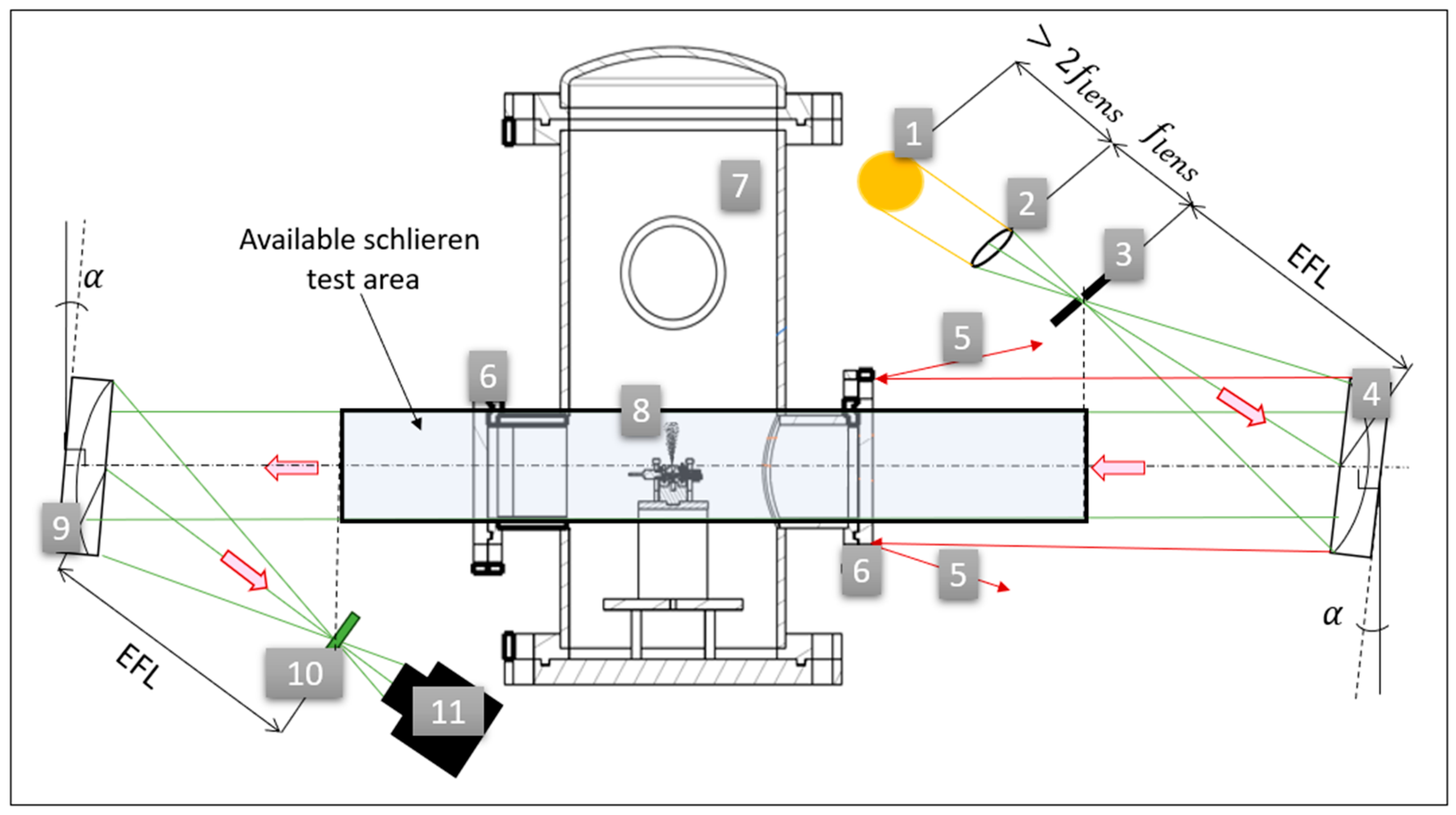
The Z-type configuration used for the imaging of the analyzed jet is presented in Figure 1, showing the optical path and the placement of the exhaust jet into the vacuum chamber. There are several rays reflected back when hitting the opaque surface of the vacuum chamber, given the fact that the diameter of the twin parabolic mirrors is larger than the visualization windows with which the vacuum chamber is equipped. The light travels from the square light source to a biconvex lens with the focal length $f_{lens}=250 \mathrm{mm}$, placed at a distance longer than he double of the focal length. Afterwards, the rays are cut in the focal plane by a square 3D printed diaphragm, which allows the passing of the light through a 1mm square area. The light from the diaphragm placed at a distance equal to the effective focal length (EFF = 1524 mm) of the parabolic mirror, reaches the first parabolic mirror, and is collimated throughout the testing area. The second mirror images the light source in its focal point, creating the knife edge plane. In the plane of the knife edge, an optical transparent filter with a color gradient distribution is framed into a calibration mechanism. The camera is placed behind it, at the point where the mirror is seen as fully illuminated. The angle $\alpha$ represents the off-axis rotation of the mirrors. In this study, $\alpha =10°$, which is more than the recommended amount ($\alpha =3°$) found in the literature [2], given the special geometrical constraints. However, the optical errors resulting from the system are visually negligible, the image of the source does not present any astigmatism or coma effects. The distance between the two parabolic mirrors is larger than 3 times their EFL, resulting in a generous testing area, while introducing the disadvantage of reducing the resolution of the Schlieren image, given the type of the camera lens used and other alignment difficulties.

The optical filter is designed according to the next equations for the RGB channels of the image. These equations are the same as the ones used by Elsinga [5], with the difference that the filter is manufactured in a different manner and the experiment positioning regarding the filter is considered to be $x_f$ and $y_f$ representing the x and y as generated by Matlab 2020a in the process of creating the image of the filter (rows and columns).

$$R=\frac{255}{1+x_f+y_f}$$

(1)

$$G=\frac{255·x_f}{1+x_f+y_f}$$

(2)

$$B=\frac{255·y_f}{1+x_f+y_f}$$

(3)

The filter was manufactured by exposing a fine grain photographic film to the image obtained in Matlab displayed on a computer screen. This process is very similar to the one explained in [5], but the filter applied in the current analysis was used in its raw form. [5] uses a different type of technology which allows the film to become completely transparent after exposure.

Given the effect of the film on the light that passes through it, the color gradients change, and the filter’s response is no longer linear, as previously intended.

The photographic film’s structure is presented in Figure 2.

The photographic film is calibrated without removing the tint effect. The Phantom Veo 1310L CMOS camera produced by Vision Research Inc. (Wayne, NJ, USA) can record 24-bit depth images, which means it is capable of illustrating $256\times 256\times 256$ possible color combinations. The structure of the colored filter and its individual color channels as shown by Figure 2 with the film tint applied is as follows: the red channel’s values vary very little causing it to look rather constant without any variation, the green gradient intensifies from left to right, and the blue channel intensifies from the bottom to the top.

The film tint effect is replicated by considering the image of a blank portion of the film, placed in the knife edge plane. An average of the color is performed and displayed with a 60% transparency over the image of the filter. The transparent film tint is represented in Figure 2 by the real image of the blank photographic film introduced into the knife edge plane. The projection of the film is considered to be the real image transferred from the photographic film onto the camera.

3. Calibration of the Filter for Color-Calibrated Schlieren

The calibration process is achieved by translating the film with regard to the fixed light source image. The photographic film dimensions are $5 \mathrm{mm}\times 5 \mathrm{mm}$.

Figure 3a presents the calibration mechanism used for translating the filter. The calibration mechanism is composed of a fixed part, and the displacement plate which contains the optical filter. This mechanism allows the displacement of the filter in 25 positions; therefore, the coverage of the entire filter can be assumed. For each position, the system will acquire information about the color ratio of each pixel. Figure 3b represents the color filter mounted into the calibration plate, while also displaying the calibration grid. Each node of the grid marked by a red cross represents the position of the light source image center, following displacement, and every white square represents the position of the light source related to the new position of the filter.

Figure 4 depicts the device placement diagram of the color-graded filter. In this case, the horizontal arrows represent a one-hole shift in the indicated direction and the vertical arrows represent the lowering of the calibration plate by one hole. The diagram starts and ends with the filter positioned in the center of the light source which can be used to detect displacement errors appearing during the calibration process. The fixing pins are represented by dark circles in order to confirm the overlap of the holes found in the calibration plate and the fixed plate.

The calibrating procedure is very similar to the one found in [5]. The displacement is achieved by starting with the colored filter in the center position and afterwards displacing it into the other 24 positions, recording different color gradients for each pixel in the 25 points mentioned. The analyzed images are recorded with the image of the light source placed in the center of the graded filter, which can be considered to be the initial position of the filter.

Figure 5 presents the initial moments of the jet development. This sequence is presented here for two important reasons. The first one is to observe the influence of the vacuum chamber on the jet’s development, illustrating the velocity with which the pressure wave returns, which can be similar to the velocity of the jet returning into the main visualized area as background noise, and the second one is to underline that the black gradient pictured into the first frame containing the jet is caused by the system recording a ray deflection angle which surpasses the system’s capabilities.

For the reason described above, the analyzed pair of images will be chosen to contain the fully developed exhaust jet in air, where the density gradients are in good correlation with the system’s sensitivity.

The system’s theoretical sensitivity in this case can be calculated using the equations used by [5], and applying it to the current case. The first step in calculating the theoretical sensitivity is to calculate the range of the displacement angle which can be recorded by the system, ${ϵ}_{range}$. This is defined as the ratio from Equation (4) [5], where $b_f$ represents the dimension of the filter, $b_s$ represents the dimension of the source, and f represents the focal length of the second parabolic mirror.

$${\epsilon }_{range}=\frac{b_f-b_s}{f}$$

(4)

The resulting ratio value is 2.6 mrad, but the ${\epsilon }_{range}$ is equal in each direction, given the square light source and filter. The displacement range is, therefore, [−1.3 mrad, 1.3 mrad]. Equation (4) confirms the hypothesis that if one uses a filter with a larger dimension, the overall detectable displacement range increases. For example, for the 12 mm × 12 filter, ${ϵ}_{range}=\left[-3.6, 3.6\right]$ mrad. The theoretical sensitivity is related to the camera’s dynamic range, is 0.80% for the $5 \mathrm{mm}\times 5 \mathrm{mm}$ filter and 0.35% for the $12 \mathrm{mm}\times 12 \mathrm{mm}$ filter. A visual comparison of the $5 \mathrm{mm}\times 5 \mathrm{mm}$ filter and the $12 \mathrm{mm}\times 12 \mathrm{mm}$ is illustrated in Figure 6.

The low resolution of the Schlieren images is caused by the issues arising from the alignment of the system. Other filter manufacturing techniques with using more modern technology such as printing the filter on a transparent laser printer sheet were discarded, as it did not allow enough light to properly pass through it because of the ink opacity, despite it seeming perfectly transparent when held against natural light.

This paper describes the calibration method and the study resulting from using the $5 \mathrm{mm}\times 5 \mathrm{mm}$ Schlieren filter. Despite the initial images presenting dark areas, the images of the analyzed jet contain pixels with color ratios which could be matched to the ones found on the above-mentioned filter. The calibration method yields for each pixel a calibration curve. These calibration curves are exemplified in Figure 7 for 3 pixels of the test image, found at the following locations: [320, 294], [321, 295], and [322, 296]. These can be described as being in the Schlieren area, in the vicinity of the thruster’s exit. Each calibration curve can be described in relation to two different color ratios, the indicated ones in this case being R/G and B/R. These pixel color ratio values exemplified in Figure 7 are obtained from the filter calibration, without the image of the studied jet. The calibration curves present five inflexion points due to the calibration mechanism and filter structure which cause an abrupt change in color ratios five times, as the filter is lowered relatively to the light source.

The deflection of the rays on the calibration filter results in a deflection angle which can be calculated for the reference image, as well as for the image containing the studied jet. The graph pictured in Figure 7 provides a glimpse into the differences between the initial design of the filter, which is assumed to only project linear changes over a single-color ration, and the color ratio distribution obtained from the physical filter obtained. The explanation of the unpredicted behavior of the filter color ratios is that the image of the filter is polluted with the film tint and there are differences between the image created in Matlab and the one displayed by the computer screen. This translates into a variation of the B/R and R/G curves, different than expected.

The deflection angle of the rays in the source image plane is considered to be split in the two directions of the Schlieren image, with ${\epsilon }_x$ and ${\epsilon }_y$ corresponding to the x and y directions, respectively. The deflection angle results from the calibration function, which in this case is written in the form presented by Equation (5).

$$\epsilon =c_1+c_2\frac{B}{R}+c_3\frac{G}{R}+c_4\frac{B^2}{R^2}+c_5\frac{B·G}{R}+c_6\frac{R^2}{G^2}+c_7\frac{B^3}{R^3}+c_8\frac{B^{2}R}{G^3}+c_9\frac{B{R}^2}{G^3}+c_{10}\frac{R^3}{G^3}$$

(5)

The coefficients of the calibration function are calculated, as suggested in [5], at each pixel. The calibration function and the calibration coefficients provide the means needed to extract the deflection angle.

This paper uses the principles applied by [5] and finds that, in a similar manner, a linear function is not enough to describe the color ratio progression. The calibration curves for the color ratios displayed in Figure 7 present similar characteristics, but do not perfectly overlap.

4. CFD Simulation

The CFD simulation of the jet was conducted for the velocimetry study found in [8], performed on the jet provided in the same functioning conditions. Due to the path integrated character of the Schlieren technique, the results of the CFD analysis can only be used for a comparison achieved in a wide range of density values. The error calculation is therefore performed only as a reference for the CS technique, for a more precise result, a DNS or LES simulation would be required.

5. Results

After the calibration of the filter is achieved and the deflection angle at each pixel is found, the density map is retrieved by applying Equation (6), where W is the length of the optical path and K is the Gladstone–Dale constant. The deflection angles expected to be obtained can be considered as sufficiently small for the approximation made for Equation (6). Equation (6) is used by Elsinga [5] to determine the density gradients by assuming that the gradient along the integrated path of the investigated 2D flow is constant. This equation leads the study found in [5] to a final density gradient obtained by means of a numerically solved Equation (7), where $\rho$ is the array containing the density values in each pixel and g is the array containing the x and y elements of the density at each pixel, while D is a sparse matrix which contains a second order central differencing scheme.

$$\epsilon =KW\nabla \rho$$

(6)

$$D_{ij}{\rho }_i=g_j$$

(7)

This, for a non 2D flow, introduces a considerable error. For this reason, the studied jet will be divided into five different sections. The Gladstone–Dale equation applied (8) in this study considers the change in K, which varies slightly with the wavelength of the light.

$$n=1+K\rho$$

(8)

A comparison of the averaged result obtained per section by CCS and the result yielded by the CFD simulation will also be further conducted.

Figure 8 presents the lines from which the date is extracted in order to compare the color schlieren results to those offered by the CFD analysis.

The density map of values at every pixel location, as resulted from the CCS analysis, is found in Figure 9 and Figure 10 (both curves in black). It presents the data obtained by calculating the density for each resulted $\epsilon$.

The results obtained through Schlieren CCS present a generally good accuracy in the 0–31 mm area, between 2% and 10%, given the position of the filter and the displacement recorded in this point. There are some pixels which present a dark character, and the explanation for those are that the filter’s dimensions were too small, the deflection angle created by the system was too big, causing the rays to land outside the filter, in a dark area. For these pixels, no density value could be retrieved. The measurement provides a good coherency with the CFD simulation in the area starting at the origin and ending at 31 mm on the x axis. After the 31 mm, the error increases dramatically and the measurement becomes irrelevant. Between line 1 and line 3, the general accuracy of the measurement is 75, when reported to the CFD result, and over line 4, the ratio of quantifiable/unusable pixels is too low to properly describe the flow. However, central axis measurements prove to be less accurate when related to the CFD results than the horizontal samples. This can be caused by many experimental factors, like the one previously mentioned (the 3D character of the flow, filter limitations, etc.).

The CFD simulation parameters are described in [8]. The functioning conditions of the installation are the thruster has been designed to provide a nominal value of 1 N in vacuum conditions, with an expansion rate of 50 and a nominal mass flow of 0.3 g/s. The thruster’s geometry consists of a convergent–divergent nozzle. Its minimal section is less than 1 mm.

ANSYS CFX was used to estimate the thruster’s performance and determine the magnitude of the flow field at the thruster’s outlet. A 3D model was created to replicate the combustion chamber’s outlet and the convergent–divergent nozzle. Figure 11 presents the conic wall used for lowering the computational demand, as the flow around the external geometry of the thruster is not considered of importance. The computational model’s dimensions are determined by the experimental chamber dimensions, which has a cylindrical geometry [8].

ICEM was used for designing the numerical grid, which has a hexahedral structure with a smaller dimension in the thruster’s inside volume and the vicinity of the thruster outlet, as can be observed in Figure 12. The grid independence was checked in terms of resulted y+ values, which were in the suggested intervals for the turbulence model used [8].

The numerical case was set based on measurements for the respective test, and thus the total mass flow was set at 0.27 g/s. In order to reduce the complexity of the numerical simulation and lower the computational demand, the combustion process was not modeled. The combustion process was considered complete at the volume inlet, with the working fluid composed of water vapor forming the complete reaction of gaseous H₂ and O₂. The temperature was determined using CEARun software (last updated in January 2023) for a stoichiometric reaction of gaseous hydrogen and oxygen resulting in a value of 3450 K. The fluid used for this simulation was a mixture of H₂O, H₂, O₂, and N₂ in order to simulate the interaction between the water vapors and ambient air [8].

The boundary conditions for this study are presented in

Table 2. Boundary conditions [8].

Type	Location	Details
Inlet	Thruster inlet	Mass flow = 0.27 g/s Total temperature = 3450 K
Wall	Thruster walls, testing chamber walls	Adiabatic walls with no slip conditions
Opening	Testing chamber outlet	Temperature = 25 °C Pressure = 1 bar

. Inlet boundary conditions were set for the thruster inlet (fixing the mass flow, total temperature and chemical components of the fluid, water vapor in this case), opening conditions for the fluid volume outlet (fixing the temperature, pressure, and chemical components). For the thruster and experimental chamber walls, adiabatic no slip conditions were used. Reynolds-averaged Navier–Stokes (RANS) simulations were conducted using the K-ε turbulence model due to its known performance for high-turbulent flows [8]. Figure 13 presents the density and temperature maps obtained from the CFD simulation.

To obtain a temperature map from the density map obtained by Schlieren, the equation of state can be applied to each value, individually. However, this will most likely present a greater error than the one obtained for the density map, as the calculation basis will already be flooded by errors, caused by the shortcomings of the method, such as the path integrated character of the turbulent axisymmetric jet, the filter’s reduced dimensions which reduces the filter’s sensitivity, and the 1pixel error introduced by the spatial resolution limitations. The temperature profile presents a 12% error in the 0–31 area and is inconclusive in the upper stages, which renders the temperature measurement by CS in this case futile.

6. Conclusions

The color-calibrated filter Schlieren (CS) method has been previously used for obtaining density maps and other parameters of 2D flows, representing a very powerful tool, registering errors from 2% to 3%, according to [5]. This paper addresses its use on 3D flows, and exemplifies a simple and low-cost method to manufacture and implement such a filter. Although the idea of using a photographic film has been around for years, the calibration mechanism has never been exemplified. The errors introduced by the filter are separated from the images the moment the filter is calibrated experimentally. For the horizontally place line A, depicted in Figure 8, the density graph reveals the issue of the jet’s symmetry, which is affected by one of the vacuum chamber’s windows, which causes the flow to propagate a little to the left of its central axis. Apart from the slight asymmetric density profile of the jet, the density curve on line A, the experimental density curve follows closely the CFD curve, with a clearer gap between the two curves values as it comes closer to the center line. This could be caused by the 3D character of the flow, which integrates the path and can cause an imprecise reading. Unfortunately, the experimental data are also scarce due to the above-mentioned pixels, where the deflection angle is large and information could not be extracted from. The measurement error was calculated by relating each experimental value to its CFD correspondent and eliminating the highest and lowest resulted error. This yielded a percentage of 2–3% on the A line.

The method can be improved with regards to the 3D flow by using a better fitted color filter, with a better color distribution. The easier way to achieve a better-known color ratio distribution would be to use a transparent step filter manufactured from gelatine sheets, like the ones produces by COMAR [9]. If the filer is cut into small sheets with a well-known length, the calibration process can be very similar to the one proposed by [5].

Corrections regarding the path-integrative character of the flow can be achieved by performing an inverse Abel transformation if the study can be considered to be propagating in a symmetrical manner.

A study in progress at this moment includes using a step color filter and applying an inverse Abel transformation, while relating the obtained measurements to the ones recorded by physical temperature sensors introduced into the flow.