1. Introduction
Argon is a noble gas, and on earth, its isotopic composition is 99.6%
40Ar, 0.34%
36Ar, and 0.06%
38Ar. Argon is very stable and chemically inert under most conditions. Due to those properties and its low cost, argon is largely used in scientific and industrial applications. For instance, in high-temperature industrial processes, an argon atmosphere can prevent material burning, material oxidation, material defects during the growth of crystals, etc. Due to its molecular simplicity (monoatomic and quasi-spherical geometry), argon is also considered a reference fluid with well-known properties, i.e., its triple-point temperature (83.8058 K) is a defining fixed point in the International Temperature Scale of 1990 [
1]. Its simple fluid characteristics allow, for example, to understand the fundamental mechanisms of interaction between ions and neutral species and thus gain a deeper insight into ion transport regimes (e.g., [
2]). The widespread use of argon requires accurate knowledge of its thermodynamic properties in the largest possible temperature and pressure ranges, i.e., covering both stable and metastable states. Numerous empirical equations of state can be found in the literature, but most of them cover only small parts of the fluid region. For example, Shamsundar et al. [
3] have shown that the development of cubic-like equations of state provides very accurate thermodynamic properties of liquids on the coexistence curve and in the metastable (superheated) state. However, this approach has flaws on the vapor side. A very detailed overview of argon’s experimental thermodynamics and the most important equations of state published prior to 1999 can be found in [
4], so we will not delve into it here. In [
4], Tegeler et al. also describe a new equation of state for argon that covers a very wide range of the fluid phase and will serve as the reference equation of state for this study.
The development of the equation of state generally starts by an empirical description of Helmholtz free energy F (i.e., an arbitrary set of mathematical functions is a priori chosen) with two independent variables: density ρ and temperature T. All thermodynamic properties of a pure substance can then be obtained by combining derivatives of F(ρ, T). The dimensionless Helmholtz free energy is commonly split into a part , which represents the properties of the ideal gas at given temperature and density, and a residual part , which takes into account the dense fluid behavior. While statistical thermodynamics can predict the behavior of fluids in the ideal gas state with high accuracy, no physically founded equation is known that accurately describes the actual thermodynamic behavior in the whole fluid region. Thus, an equation for the residual fluid behavior, in this case for the residual part of Helmholtz free energy , has to be determined in an empirical way. However, as Helmholtz free energy is not accessible to direct measurements, a suitable mathematical structure and some fitted coefficients have to be determined from properties for which experimental data are available. Hence, all the physical properties are contained in the mathematical form given to Helmholtz free energy.
In the wide-range equation of state for argon developed by Tegeler et al. [
4], the residual part of Helmholtz free energy
contains polynomial terms, Gaussian terms, and exponential terms, resulting in a total of 41 coefficients (named
ni in [
4]), which represent the number of mathematically distinct entities (with each mathematical entity containing several adjustable parameters). This equation of state is valid for the fluid region delimited by
and
The large number (~120) of adjustable parameters of the equation of state of Tegeler et al. (see Table 30 in [
4]) are determined by a sophisticated fitting technique that is a powerful mathematical tool and a practical way for representing data sets (by assigning weights to each of them subjectively). This technique provides an easily practical overall numerical representation of the data, but it also allows for the completion of the representation of measurable quantities in areas where no measurements have been made. However, passing in a set of data points does not mean that the obtained variations have a physical meaning or that the physical ideas underlying mathematical representation are unique. For example, the following drawbacks of the equation of state of Tegeler et al. [
4] can be noticed:
Extrapolation of the equation for the isochoric heat capacity in regions of high or low density and high temperature is non-physical.
The extrapolation of polynomial developments does not generally give valid results; indeed, polynomial development is very sensitive (i.e., instable) with respect to the values of its coefficients, and these coefficients cannot be truncated, even slightly. Therefore, all the coefficients
ni of Tegeler et al. [
4]’s model have 14 digits, and the coefficients thus have no physical sense.
The model applies to the pure fluid phases and cannot, in its actual form, take into account particular properties inside the liquid–vapor coexistence region. Moreover, the model gives negative values of CV on some isotherms inside the liquid–vapor coexistence region (CV < 0 is never observed for classical thermodynamic systems). This implies, for example, some non-physical variations in the liquid spinodal curve.
The aim of this paper is not to increase the precision of the equation of state of Tegeler et al. [
4] in its own domain of validity but instead to develop a new equation of state based on different physical ideas that can fill the drawbacks previously expressed in order to obtain a more physical description of the experimental thermodynamic data of argon in a broader temperature and pressure range. In the classical approach, the ideal part of the free energy is generally determined from the well-known properties of the ideal gas heat capacities. We propose to also extend the classical approach to the residual part; therefore, the proposed new equation of state is based on an original empirical description of the isochoric heat capacity
CV(
ρ,
T) containing the metastable states explicitly. Then, the thermodynamic properties (internal energy, entropy, and free energy) are obtained by combining the integration of functions involving
CV(
ρ,
T). For instance, internal energy
U can be deduced from
, where
U0(
ρ) is an arbitrary function of density. In this way, possible data noise is smoothed. However, an integration process introduces arbitrary functions (e.g.,
U0(
ρ)). These functions can be deduced from a comparison between calculated and experimental data. The pressure equation of state
P(
ρ,
T) was chosen because it is the largest available data set. The set of experimental data taken into account by the model of Tegeler et al. [
4] will be further extended with the inclusion of the L’Air Liquide database [
5], thus extending the temperature validity range of this new modeling compared to that of Tegeler et al. The interest of this new approach is that it can be easily extended to all other fluids that exhibit a first-order transition with metastable states.
Hereafter,
the model of Tegeler et al. [4] will be simply named the TSW model. 2. A New Equation of State for Isochoric Heat Capacity
As stated previously, the present approach starts with the empirical description of a chosen thermodynamic quantity. An experimentally measured quantity is chosen for description, which is not the case for Helmholtz free energy. The quantity that has the simplest mathematical and physical comprehensive variation is the isochoric heat capacity
CV as a function of density
ρ and temperature
T. Starting with this quantity, we therefore lose the advantage of the description provided by Helmholtz free energy, from which all other thermodynamic quantities can be obtained by derivation. However, it allows us to more easily introduce new physical bases, in particular non-extensivity, and simplicity is enhanced. Indeed, the number of coefficients
αi (without
αcrit,b) for the description of
CV is 11 (see
Table 1), and it will be shown in the next section that the number of coefficients
αi for the description of Helmholtz free energy is only
26 compared to
41 for the TSW model.
After choosing the thermodynamic quantity to be described, one must find a mathematical structure for its representation. A virial-like development is an easy and widespread approximation. The problem with polynomial terms is that they introduce very small oscillations that are not physical. To avoid such effects, it is assumed that the description must not contain any form of polynomial expression. Thus, the description is formulated in terms of power laws and exponentials with density-dependent exponents. We shall see that with such a description, we obtain a dozen different characteristic densities among the parameters of the model instead of only ρc (which is consistent with the fact that argon does not follow the law of corresponding states). Therefore, all the equations of states are expressed in a dimensionless form according to the variables ρ and T, which lead to simpler expressions than if one had considered the dimensionless variables ρ/ρc and T/Tc. In addition, the most suitable units for density ρ and temperature T have been chosen as g/cm3 and Kelvin, respectively.
As for Helmholtz free energy, the isochoric heat capacity is split into a part
, which represents the properties of the ideal gas and a part
, which takes into account the residual fluid behavior at given
T and
ρ. Note here that the ideal part of free energy is, in fact, determined by the known properties of
in the classical approach. Because argon is monoatomic, only the translational contribution to the ideal gas heat capacity
has to be taken into account, so it is deduced from Mayer’s law that
. In dimensionless form, the isochoric heat capacity is written as follows:
To take into account all fluid domains, including the liquid–vapor coexistence region and the region around the critical point,
must be split up into three terms—regular, non-regular, and critical—such that
with
where
λ = 6.8494 and
,
,
,
,
, and
are empirical functions determined from the best fit of NIST [
6] and Ronchi [
7] data, whose expressions are given further on. In other words, it is assumed here that these two data sets are a priori consistent with each other.
An important feature of the Ronchi model is to predict the appearance of a maximum on the isochoric heat capacity CV along isochors. A maximum of CV along isochors has been experimentally observed in several fluids, for example, water. Consequently, the extrapolation of CV along isochors from a given model must show a maximum, as predicted by the Ronchi model. This predicted behavior of CV along isochors constitutes the main interest of the Ronchi model.
The Ronchi calculated data cover the largest available temperature range of 300 to 2300 K and the largest available pressure range of 9.9 to 47,058.9 MPa (420 data points). It is important to notice that they are consistent with many experimental data that were used by Tegeler et al. [
4] but which they assigned to groups 2–3. The data of Ronchi were assigned to Group 2 by Tegeler et al. From the data of Ronchi, the highest available density is called
ρmax,Ronc, and its value is given in
Table 2.
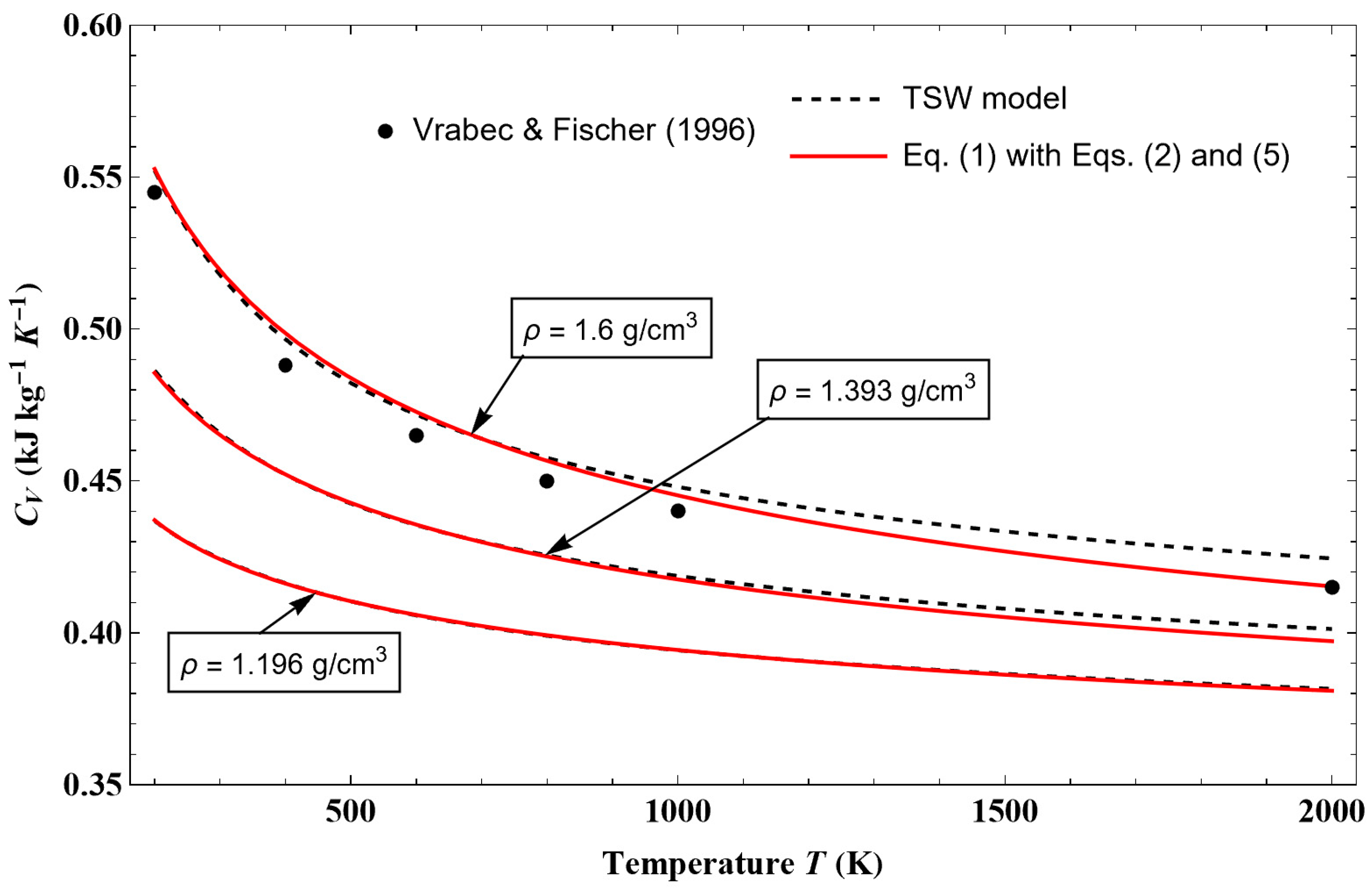
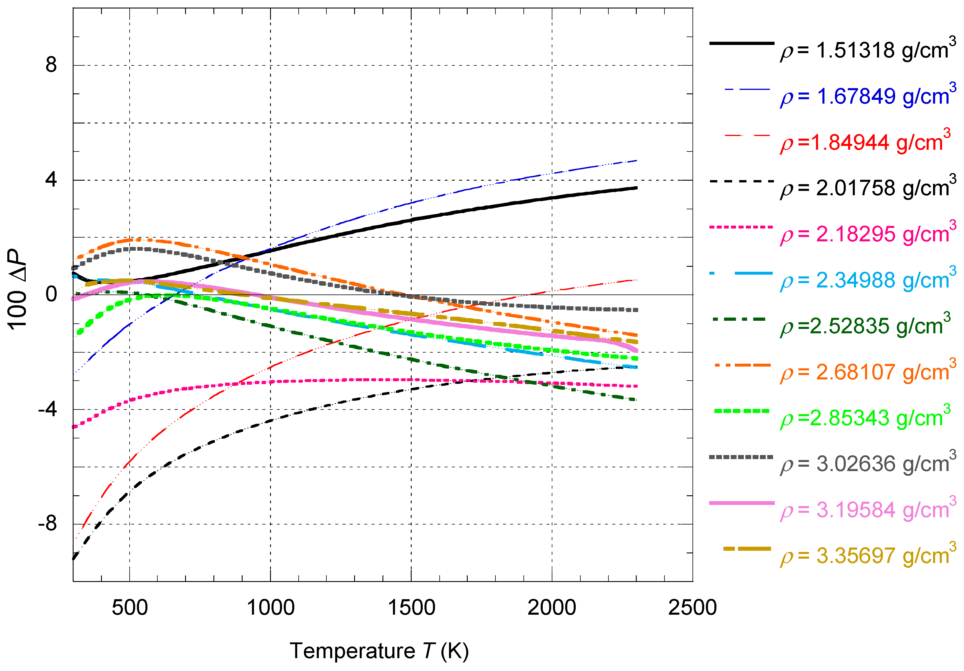
By construction, a part of the Ronchi [
7] and NIST [
6] data overlaps. For their common range of density values, it is observed in
Figure 1 that the deviation is always less than 2.5%, so the data of Ronchi can be considered to be consistent with the data from NIST.
Hereafter,
the term “NIST” will simply be used to refer to the data in [6] and the term “Ronchi” to refer to the data in [7].The relations constituting Equation (2) are therefore consistent with two sets of coherent data, but at this stage of the theoretical development, it must be strongly emphasized that these relations are only valid for temperatures
T ≥
Tdiv(
ρ), i.e., in particular for all states in the single-phase region. In this way,
Tdiv(
ρ) defines a divergence curve (i.e., it defines an asymptotic curve), and we will see later that it is related to the spinodal curve. We shall see in
Section 3.4 how this relation is transformed for
T <
Tdiv(
ρ) (i.e., for states inside the coexistence region).
It is very important to notice that with the present model, once the mathematical form of the regular term is chosen, it is not possible to envisage any mathematical form for the two other residual terms. Indeed, the two remaining terms must have a consistent mathematical form with that of the first one; otherwise, the amplitude terms ni become erratic functions of density and are no longer smooth functions. The mathematical forms are certainly not unique, but there are strong constraints on them. This is a fundamental difference from the classical fitting approach to the free energy function, where there is no mathematical constraint between the different terms that are summed.
The three terms of the residual part of CV are now clarified.
The first term , which is a simple power law, is called “regular”. It shows no singularity and can be calculated for temperatures from Tt (triple-point temperature) up to infinity. When T → 0 K following isochors, this term can be approximated by
which tends towards zero as a linear law.
For
T >>
Tc/
λ,
reduces to
The characteristic temperature Tc/λ = 22.0 K is not the Debye temperature of argon, which is equal to 85 K. This new characteristic temperature was chosen to minimize the relative error of CV on the saturated vapor pressure curve so that the term containing λT/Tc becomes important only for temperatures smaller than the triple-point temperature (i.e., for T << Tt with λ = 6.8494).
The second term , called “non regular”, presents an asymptote for (i.e., CV is infinite for this value of temperature). This term is only significant near the liquid–vapor coexistence region. We can also note that the divergence is weak.
The third term is important only in a small region around the critical point. This term allows us to reproduce the very sharp evolution of CV very close to the critical point. It can be understood as the macroscopic contribution of the critical fluctuations. This term plays the same mathematical role as the contribution of the four last terms in the second derivative with temperature of the residual free energy in the TSW model.
We have pointed out that the regular term
tends to zero when
T tends to zero. It will be shown in
Section 3.4 that for
T <
Tdiv, the non-regular and critical terms also have a limit equal to zero when
T → 0 K. Hence,
if
T → 0; this result is in agreement with the third law of thermodynamics (Nernst–Planck assumption). Because
, this law imposes
→ 0 if
T → 0 and then
→ 0 if
T → 0. To reach this result,
is rewritten in the following form:
where
λ0 = 18.2121.
In the expression of
, all coefficients depend on density
ρ in the following way:
where
εi are exponents, and
αi are characteristic coefficients.
Table 1 lists the values of these parameters.
Note that the function is decomposed into two parts so that Equation (8) can represent Ronchi data at very high density (i.e., for ). Indeed, the variations imposed by Ronchi data are too complex to be taken into account by a single function.
Now, some explanations will be given for the properties of these coefficients. Most of them involve the three characteristic densities of argon:
the density of liquid at the triple point;
the density of gas at the triple point;
the critical density .
Moreover, two other characteristic densities,
and
, have to be added in view to correctly fit the data of Ronchi at very high densities. All values of these characteristic densities are given in
Table 2.
Obviously, other mathematical forms for Equations (6)–(12) could be used, but the proposed equations are the simplest ones that have been found and that lead to an accurate fitting of the whole data set. The consequences of this representation will be seen in
Section 3.1.
The density dependence of the
ni coefficients is shown in
Figure 2. Each coefficient is equal to zero when
ρ → 0 and
ρ → ∞ and gets through a maximum in between (the maximum of
nreg really occurs but is outside the range of density shown in
Figure 2).
The density dependence of exponent
m is shown in
Figure 3. This coefficient is always strictly smaller than one, and it tends to −∞ when
ρ → 0 and
ρ → ∞. Then, there are two density values for which
m = 0. This means that, in the region where
T >>
Tc/
λ,
is always decreasing along isochors when the temperature is increasing.
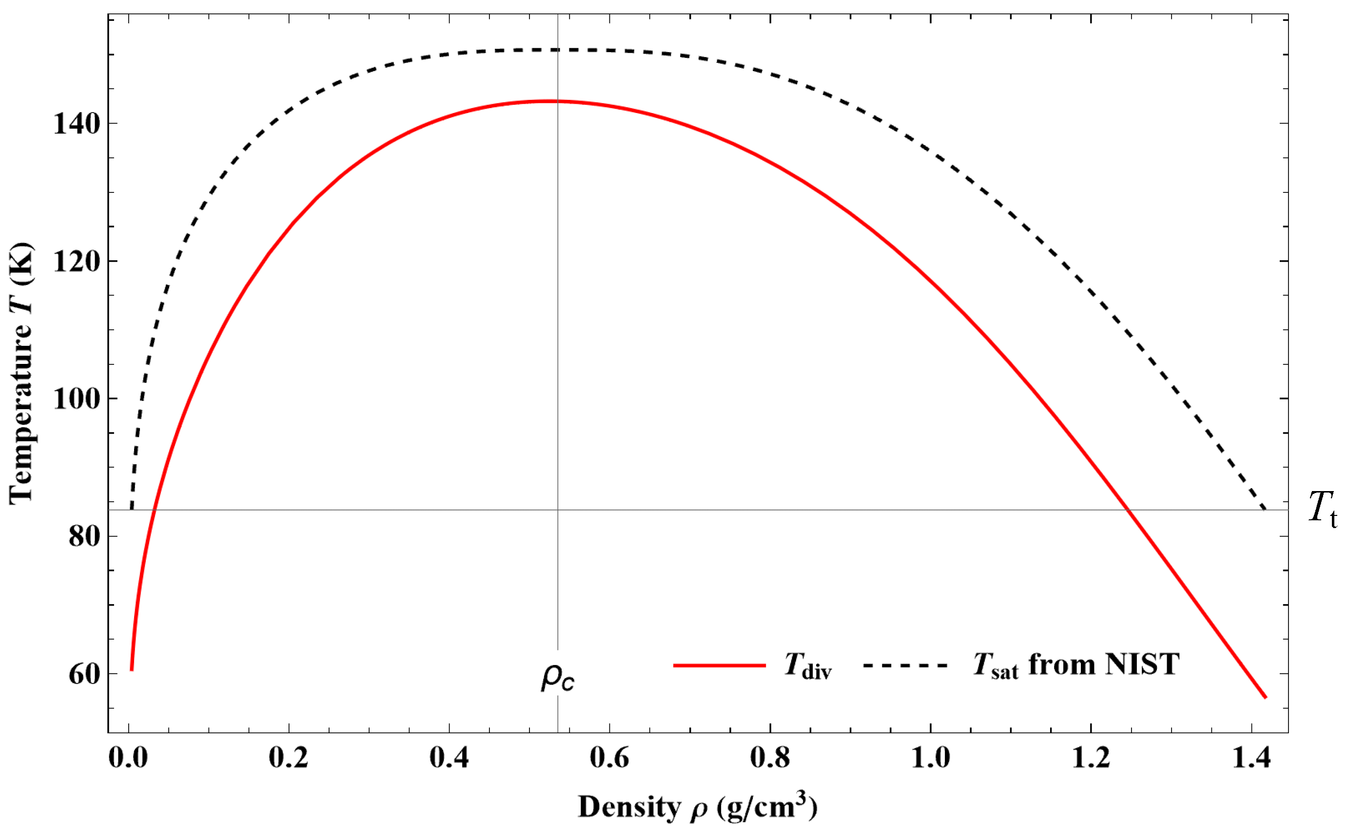
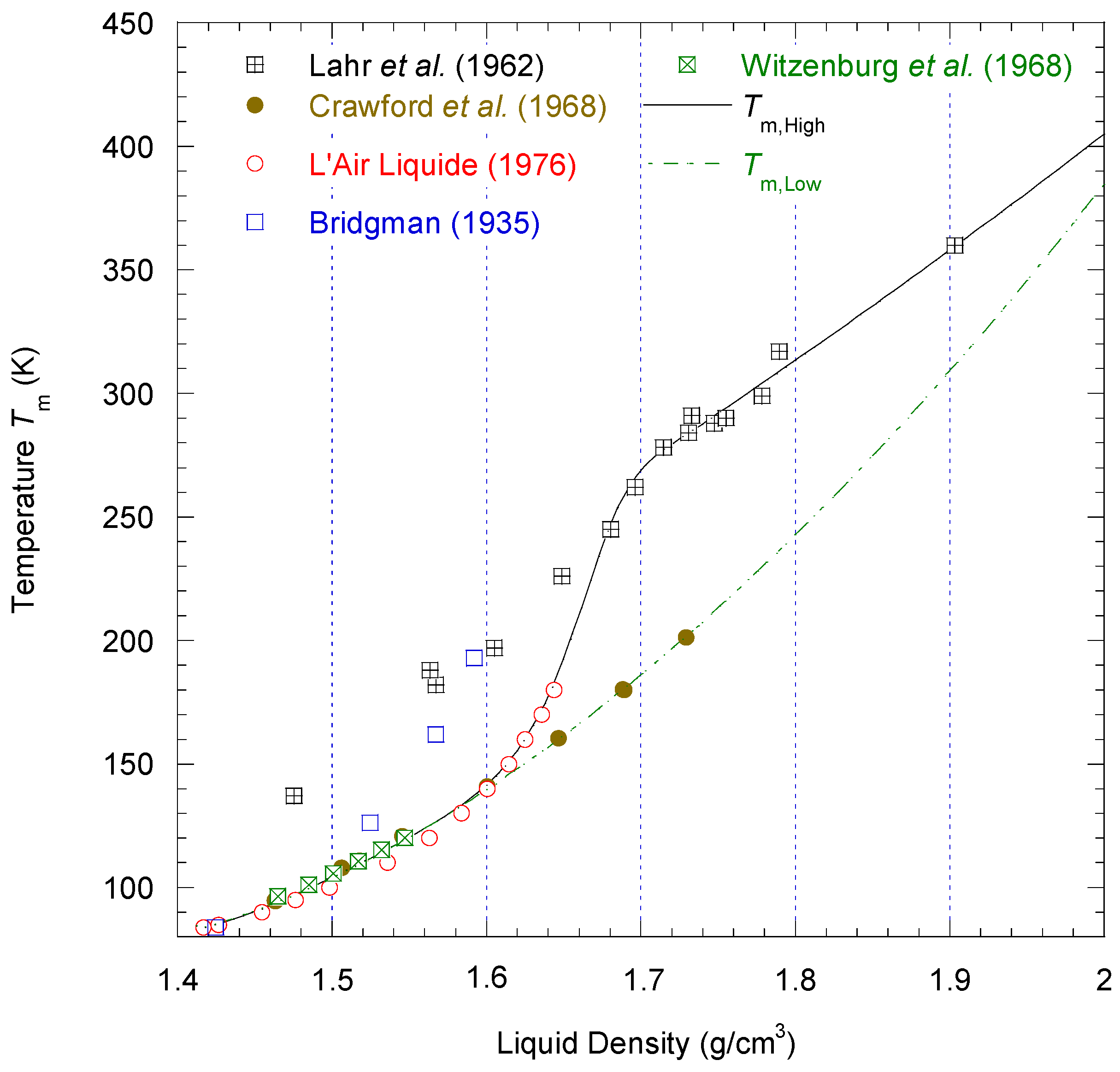
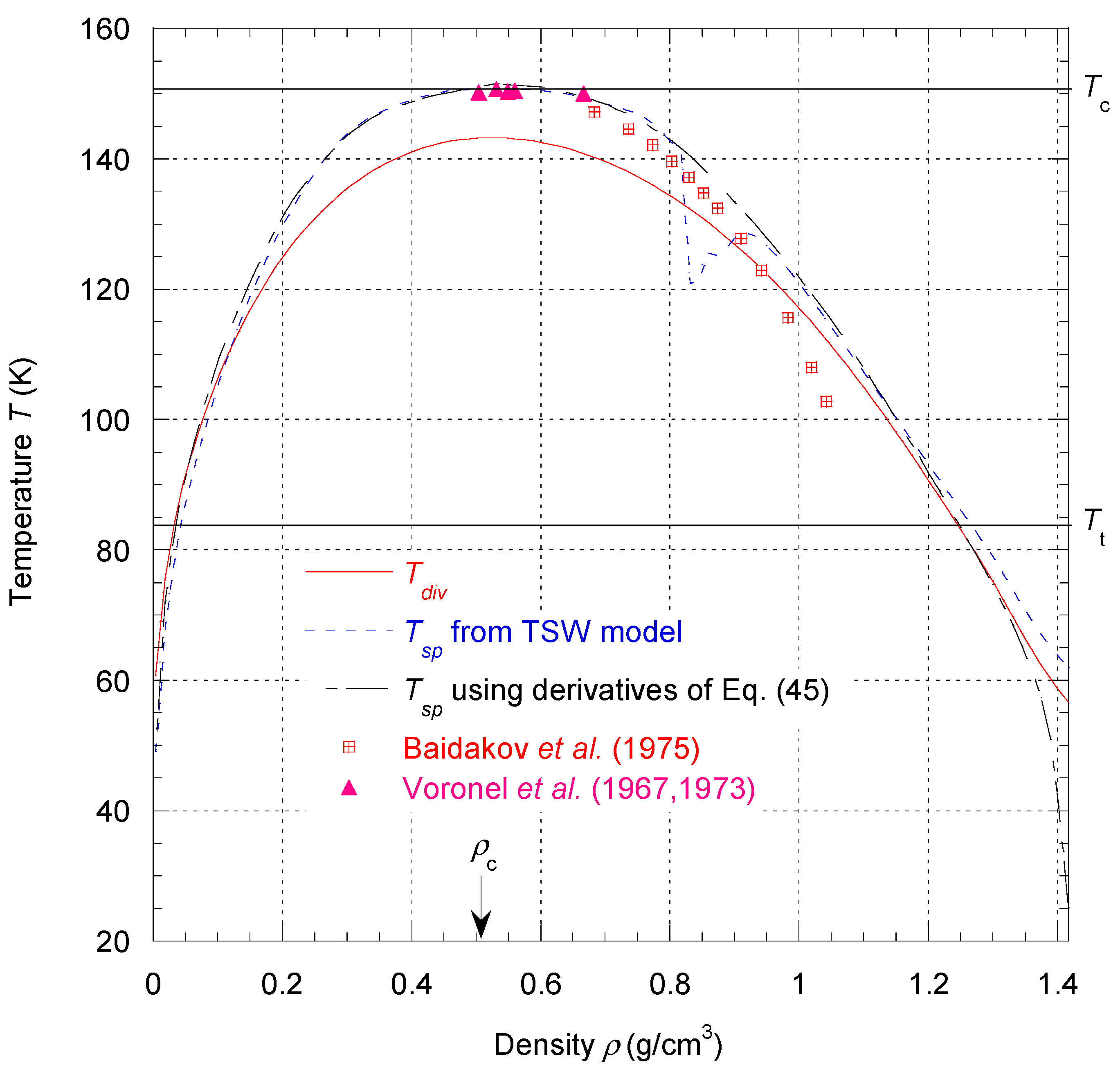
The characteristic temperature
Tdiv as a function of density defines a curve
that lies entirely inside the vapor–liquid coexistence region defined by
(see
Figure 4). For a first-order phase transition, the divergence of
CV must occur on the spinodal curve (i.e., loci of thermodynamic mechanical instability), corresponding to
Because no experimental data of the spinodal curve can be found in all the density ranges from
to
,
Tdiv was only determined by fitting the data of
CV from NIST. If this set of data is accurate and consistent enough with the
PρT data set, one should be able to identify
as the spinodal temperature curve. We will discuss the results obtained for the spinodal states in more detail in
Section 4.3.3.
From Equation (2), it is also easy to see that the second thermodynamic instability (i.e., the thermal instability), defined by
will never occur in the present approach, contrary to the TSW model.
Consequently, with Equation (2) being valid for
T >
Tdiv, this relation can be used in the vapor–liquid coexistence region by crossing
till approximately the spinodal curve. No trouble occurs as long as
T >
Tdiv, though the model is based on a pure fluid description. The fact that there is no discontinuity of
CV when crossing the coexistence curve (except at the critical point) is a characteristic of a first-order transition. We shall see in
Section 3.4 how to treat the crossing of the divergence curve defined by
. Finally, it can be noticed that
Tdiv = 0 for
ρ = 0 and
Tdiv → 0 when
ρ → ∞; hence,
shows the right density dependence, which allows us to investigate the fluid properties from the gas phase up to the sublimation curve.
The flexibility of the present method is now illustrated from the equation of state for the isochoric heat capacity. If one wants to represent the data from NIST instead of the data of Ronchi for densities higher than
, it is only necessary to change the values of the couple (
ρreg,Ronc,
) and the mathematical form of the exponent function
m(
ρ). In this case, Equation (7) must be replaced by the following function:
with
where
represents the exponential integral function. The corresponding parameters have the following values:
- -
Coefficients: αm,1 = 0.48962315, αm,2 = 0.24014465, αm,3 = 1.0932969, αm,4 = 0.08936644, αm,5 = 67.4598, and αm,6 = 1331.29.
- -
Exponents: εm,3a = 1.56671, εm,3b = 0.930273, εm,4 = 4.785, εm,5 = 166.594, εm,6 = 5.93118, and .
- -
Characteristic densities in g/cm3: ρm,2 = 1.35802, ρm,3 = 0.449618, ρm,4a = 3.30149, ρm,4b = 4.05911, and ρm,6 = 24.5967, and the new value for ρreg,Ronc is now equal to 2.22915.
It immediately follows that this new function needs more parameters than for Equation (7), but the global shape of the function is very similar to that of Equation (7), except that this new function has a strong oscillation around the density value ρ = 1.8 g/cm3. This oscillation is needed for a good representation of the data, but it is physically difficult to understand. Equation (7bis) is therefore of no practical use compared to Equation (7) and will not be analyzed further.
3. Thermodynamic Properties Derived from Isochoric Heat Capacity
Because Helmholtz free energy versus density and temperature is one of the four basic forms of an equation of state, we focus here on the process for deducing its expression. For this purpose, we used the thermodynamic relation:
Consequently,
F can be deduced from (i) two successive integrations of
CV or (ii) a single integration of
CV to calculate
U and
S and then use the thermodynamic relation:
with
,
and
(given by Equations (1), (2), and (5)).
We chose the second approach that the two integrations to find
U and
S induces the existence of two arbitrary functions,
U0(
ρ) and
S0(
ρ), respectively, which are simpler to determine than directly finding the arbitrary function for
F. The later simply writes
F0(
ρ,
T) =
U0(
ρ)
− TS0(
ρ). It will be seen in
Section 3.1 how the two arbitrary functions
U0(
ρ) and
S0(
ρ) can be determined.
There is no difficulty in finding a primitive of
for
U or
S. For the residual part of
CV (see Equation (2)), there is also no difficulty in finding a primitive of
and
. However, for
, when
T >>
Tc/
λ, two expressions can be obtained for the primitive of
U depending on whether the value of
m(
ρ) is zero or not, that is to say, a power law if
m ≠ 0 and a logarithmic law if
m = 0. It can be seen in
Figure 3 that there are two values of
ρ for which
m = 0, namely,
ρlow = 0.11726382 g/cm
3 and
ρhigh = 3.29510771 g/cm
3. To obtain a single expression that is uniformly valid, the primitive is written as follows:
Using the Hospital’s rule, it can be easily verified that , which corresponds to the right expression for the primitive when m = 0.
The same problem occurs for the primitive of S, but this time, the expression depends on whether m = 1 or not. For argon, the value m = 1 is never reached, but to maintain a general expression, we proceed in the same manner to determine the expression for the primitive of S.
For the integration of
CV, the only term for which it may be difficult to find a primitive is
(see Equation (2)). It could be integrated numerically, but a reference state must be chosen; this will be shown in
Section 3.4. To find a primitive, it is also possible to perform a series expansion of the term
with
. Hence,
can be written in the following form:
A primitive for each term of the series can be obtained. For a practical calculation, the series expansion must be truncated. The convergence is slower as
x approaches the unit value, and as a result, the number of terms that must be considered increases. An empirical formula for calculating the number of terms required is given below so that the residual error due to truncation is less than 0.1% (except for
x > 0.99 because the function weakly diverges as
T →
Tdiv):
where
represents the integer part function.
Finally, the equations for
U and
S can be written in standard dimensionless form (i.e., an ideal gas part and a residual one) as
with
and
with
where
represents the incomplete gamma function, and
represents the exponential integral function.
In the ideal gas limit, the relations for internal energy and entropy must be written as
where
and
are arbitrary constants. These formulas can be rewritten as follows (using Equation (5) for
):
Equations (26) and (27) are used to express the Helmholtz free energy and its various derivatives as shown in
Table 3.
The above expressions can now be used to rearrange Equations (20) and (22) in order to extract the residual part for the internal energy (i.e.,
minus the ideal gas part) and for the entropy:
where
and
are two arbitrary constants. In view of fitting NIST data, the constant values must be such that
and
.
3.1. Determination of the Arbitrary Functions for Internal Energy and Entropy
The two arbitrary functions
U0(
ρ) and
S0(
ρ) can be determined in two different ways. One way is to find the difference between previously published data of
U (or
S) and the
U (or
S) values calculated by the present modeling and then find a function (
U0(
ρ) or
S0(
ρ)) that best fits this difference. However, this method could be problematic as
U and
S are not measured quantities and depend on a chosen reference state. Another way is to use a new experimentally measured quantity, namely, pressure
P, and by using the following relationship:
Along isochors, from Equations (15) and (16), it is deduced that
, and its derivative versus
V (or
ρ) gives
, with
,
, and
. Here,
is calculated from the
CV values given by Equation (1). For a given isochor of density
ρ, the difference
must be a straight line (of slope
and ordinate at origin
) if the
CV values are well predicted by Equation (1). This is effectively observed in
Figure 5, which displays
versus
T on different isochors (i.e., the quasi-infinite curvature is a consequence of the extremely good representation of
CV along isochors). The best and simplest functions that represent
and
are
and
with
Before continuing, it is worth noting that and .
A primitive of expressions (31) and (32) leads to the functions
U0(
ρ) and
S0(
ρ) such that
and
with
where
represents the exponential integral function, and erf(
x) represents the error function.
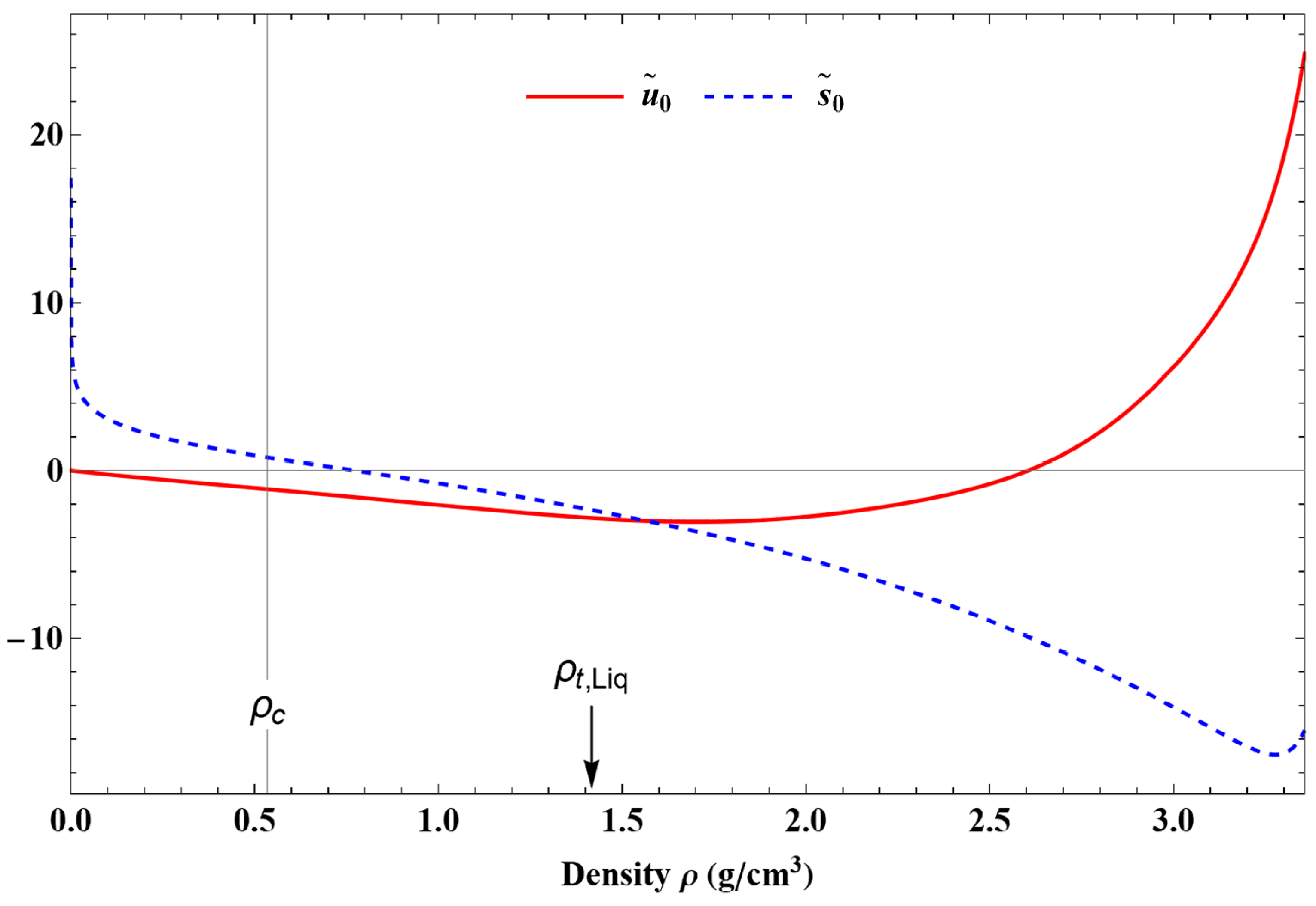
The coefficient and exponent values appearing in these equations are given in
Table 4. The density dependence of the terms
and
are shown in
Figure 6.
It is important to remember that the two primitives above depend on an arbitrary constant
and
, respectively. Moreover, it must be ensured that the dimensionless form for internal energy is such that
and for the entropy,
From Equations (20), (22), and (34)–(38), the expression for Helmholtz free energy can be easily deduced. In dimensionless form, this one writes as follows:
where
is given in
Table 3 and
with
For the sake of simplicity, the two constants
and
can be chosen such that
and
. It follows that
and
It appears that if one wants to represent the data from NIST instead of the data of Ronchi for densities higher than , it is only necessary to change the mathematical form of Equations (31)–(33). For example, the new function for can be written with the same mathematical terms as in Equation (31) but without the two last terms and with different values of the parameters. Therefore, it can be understood that the global shape of the new functions and will have very similar variations. This remark also shows that the two data sets discussed above for high densities can be represented by only small variations in the shape of the two derivative functions and . Once these two functions are determined, all the thermodynamic equations of state are known.
Table 5 summarizes the various terms making up the residual part of the Helmholtz free energy.
3.2. Analytic Expression of the Thermal Equation of State for T ≥ Tdiv
The thermal state equation
P =
P(
ρ,
T), which is a fundamental equation to calculate the basic thermal properties of argon, can easily be established using Equations (30) and (39) for free energy. Free energy is made up of four terms coming from the residual part of Helmholtz free energy and a term that represents the behavior of the ideal gas:
or in a dimensionless form
with
It is recalled that
in the expression of
.
displays too many terms, and its expression is given in
Appendix A. The expressions of the first derivatives of Equations (6)–(12) are listed in
Appendix B. From the expression of these factors, it is easy to see that
and
for
ρ → 0; therefore,
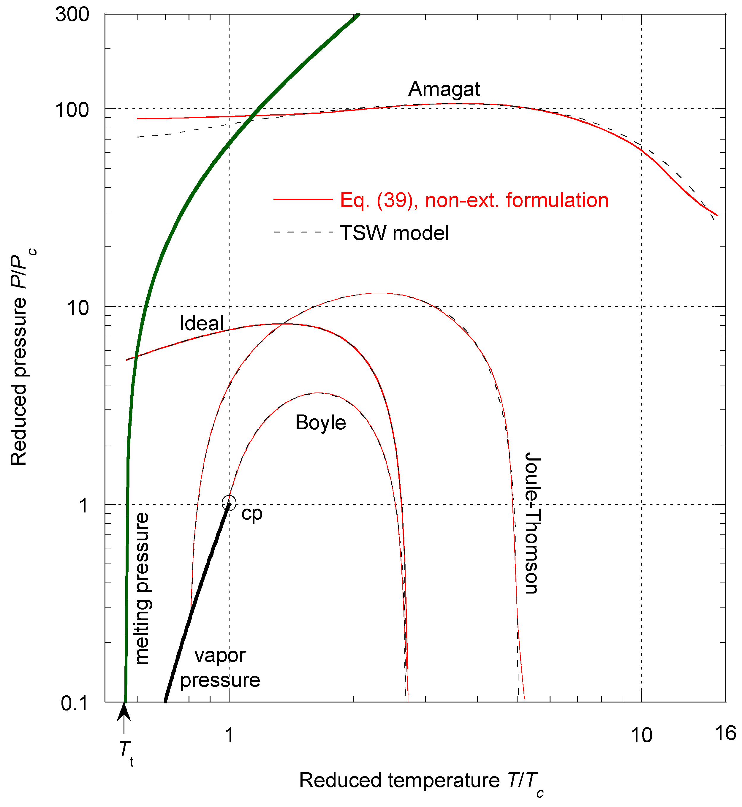
for any temperature when density tends to zero. In a certain range of temperatures, isotherms intersect the line
Z = 1 for
ρ values that are not identically zero. As thermodynamic quantities corresponding to
Z = 1 are physically important and not easy to find in the literature, they are listed in
Table 6.
3.3. The Liquid–Vapor Coexistence Curve
At a given temperature
T, vapor pressure and densities of the coexisting phases can be determined by the simultaneous resolution of the equations:
where the indices
σl and
σv represent the liquid and the vapor coexistence states, respectively.
These equations represent the phase equilibrium conditions, i.e., the equality of pressure, temperature, and specific Gibbs energy (Maxwell criterion) in the coexisting phases. The calculated values on the liquid–vapor coexistence curve (vapor pressure, saturated liquid density, saturated vapor density, etc.) are given in Table 12. Approximate formulas for representing the pressure and densities of liquid and vapor as a function of temperature along the coexistence curve are given in
Appendix C.
3.4. Thermodynamic State inside the Liquid–Vapor Coexistence Curve for T < Tdiv(ρ)
The thermodynamic properties of argon are calculated from the isochoric heat capacity equation CV(ρ, T). However, with the equation only being valid for T ≥ Tdiv, a new equation, valid for T < Tdiv (i.e., inside the liquid–vapor coexistence region), has to be established. This requires solving three mathematical problems.
First, an expression of CV(ρ, T) for T < Tdiv(ρ) has to be found.
Secondly, to integrate CV, the artificial divergence introduced with the term must be removed in order to have a finite value of CV for T = Tdiv(ρ).
Finally, for the integration of CV, a reference state must also be chosen.
The procedure used to develop the modified equation is now presented. It will be shown that this new formulation leads to a better description of the two-phase thermodynamic properties than the polynomial approach.
3.4.1. Expression of CV
The two terms in
CV(
ρ,
T) creating difficulties are
and
. For
T <
Tdiv,
becomes negative, which has no physical meaning; indeed, the thermodynamic thermal stability has always to be satisfied. And the term
, for
T <
Tdiv, diverges when
T → 0, which also has no physical meaning. The easiest way to solve these problems is to take a symmetric function by changing the variable
into
; hence, the following is obtained:
However, a problem remains as the two equations ( and ) become infinite for T = Tdiv. In fact, this is the consequence of the extensive nature of CV. Therefore, this divergence can be removed by explicitly introducing a finite number NV of particles into the equations for CV. NV has to be the largest possible without being infinite (which is the condition for an extensive property). Then, as these equations must converge for T = Tdiv, the terms and have to be corrected so that the two equations must tend to the same finite value for T = Tdiv. The following functions have the required properties:
is replaced by
, so
now becomes
and
is replaced by
, so
now becomes
The two corrections tend to
when
.
NV may be thought of as a quantity representing the number of particles in the volume
V for a given experiment, so it can be written as
where
fmol = 10
20 is an arbitrary constant required to remove the divergence. This means that, near the transition,
CV and its related quantities are no longer extensive quantities. This is not surprising because sample size effects are known to exist around the phase transition. Thus, the divergence occurs only for an infinite number of particles. This non-extensive contribution introduced in Equations (55) and (56) has also been used to revisit liquid physics in order to explain rheological behavior under a wide variety of thermodynamic and mechanical conditions [
8,
9,
10,
11].
Outside the liquid–vapor coexistence region, the percentage deviation between
calculated by Equation (18), and
, calculated by Equation (55), is shown in
Figure 7. It is observed that the difference is only significant in the close vicinity of the critical point.
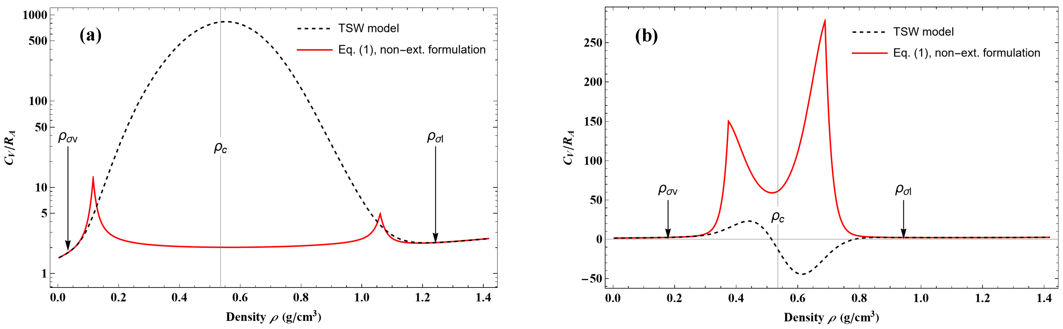
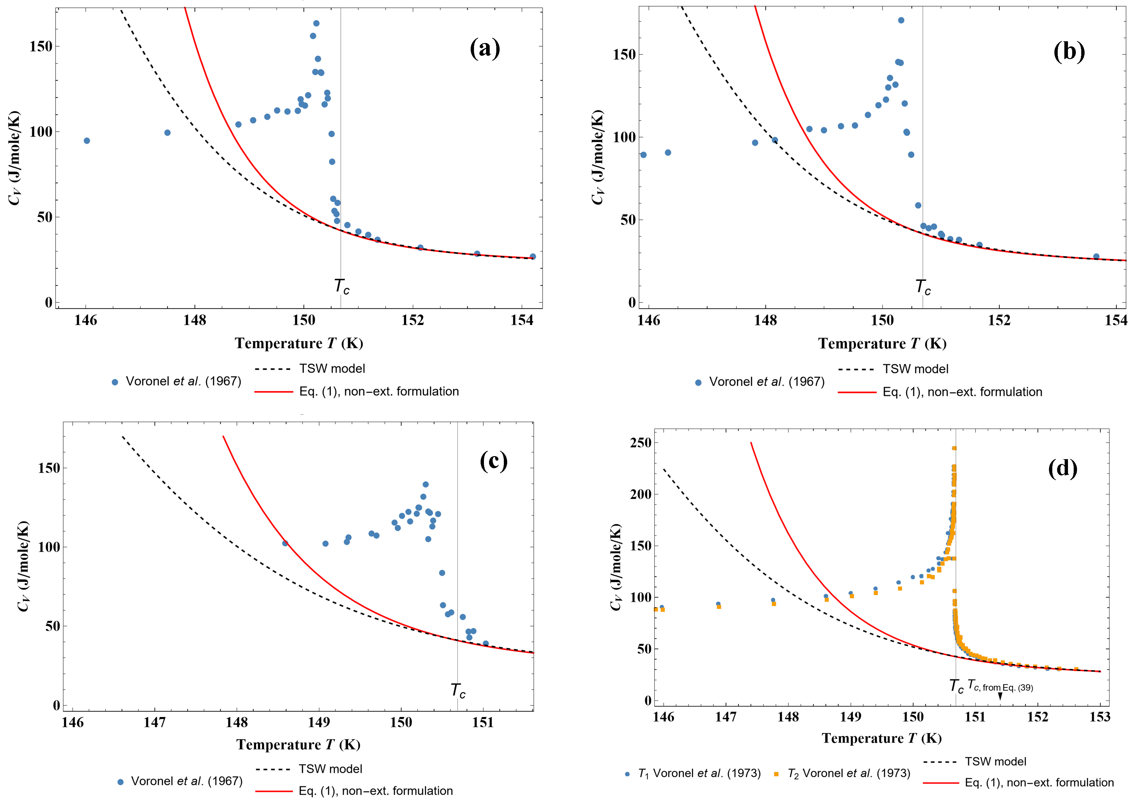
Figure 8 shows the behavior of
CV on two isotherms that are crossing the coexistence phase. One can observe that, on both isotherms, the new model always gives positive values of
CV with maximum values, as has been experimentally observed. It can be noticed that the TSW model leads to erroneous
CV variations in this coexistence region.
3.4.2. Choice of a Reference State
The functions U, S, and F are obtained by successive integrations of CV along isochors; this means a reference temperature is necessary. From Equations (55) and (56), it is obvious that the only state that is identical for all isochors is T infinite.
Due to the fact that, firstly, the development of an equation such as Equation (18) for
becomes more complex with a much slower convergence of the series and, secondly, there are two expressions for this term inside the liquid–vapor coexistence region, it is preferable and easier to numerically integrate these terms. Thus, the respective expressions for
and
are now
with
.
To complete the description, the expression for the non-regular compressibility factor is also given, i.e.,
To calculate the partial derivative of
,
NV must be considered constant because the experiments imagined here to measure the pressure are performed on a closed system. Thus, the expressions of the partial derivative of
are
In the same manner as previously, one can deduce primitives for
U and
S corresponding to the term
as follows:
Then it is deduced that
and
We emphasize here that the choice of these expressions to describe the coexistence region has no effect on the properties of the pure fluid up to the saturation curve.
The present modeling with these new expressions of regular and non-critical terms is referred to as the “
non-extensive formulation”. The non-extensive residual part of Helmholtz energy
and its partial derivatives with temperature are given in
Table 7. The first partial derivative with density can be easily deduced from the expression of the compressibility factor Z. Then, the second partial derivatives
and
can be obtained from the first derivatives of the compressibility factor, which are given in
Table 8 and
Table 9.
Table 26 of [
4] summarizes how to calculate the thermodynamic properties from the empirical description of Helmholtz free energy and its derivatives. In the present approach, the same thermodynamic properties are deduced from the isochoric heat capacity equation and the thermal equation of state, which are now two experimentally measured quantities.
A Mathematica application with the new equations of state corresponding to the non-extensive formulation can be found in the Supplementary Materials.
6. Tait’s Equation of State to Describe the Liquid Phase
As a result of Tait’s work to understand and analyze the ocean temperature measurements [
33] from the first global oceanographic campaign of the H.M.S. Challenger [
34], it was shown that most liquids can be described empirically by a so-called Tait equation of state [
35]. The most commonly used form of equation is the so-called Tait–Tammann equation, defined from the isothermal mixed elasticity modulus in volume, which we will write here using the notations of [
35] (in Chapter 3):
where
V represents the specific volume of the liquid,
the specific volume of liquid along the coexistence curve deduced from Equation (A24), and
Psat is given by Equation (A23). The two Tait–Tammann parameters
and
have the following expression in the case of liquid argon:
where
with
Tc =
Tc,non-ext. formulation = 151.396 K and
Pc =
Pc,non-ext. formulation = 49.9684 bar. Equation (72) gives
in bar, and Equation (73) gives
in cm
3/g.
It can be immediately noticed that Equations (72) and (73) verify the necessary conditions for thermodynamic stability such that
and
(see Section 3.3 of [
35]). Equation (72) implies that the corresponding temperature for which
for argon is
T∞ = 137.584 K. This temperature represents the transition between liquid- and gas-like behavior. Therefore, for temperatures
T∞ <
T <
Tc, Equation (71) shows an asymptote that lies in the biphasic region for
T < 150.5 K, but beyond that, it appears in the liquid phase. In other words, it is not advisable to use the Tait–Tammann approximation for temperatures above 150.5 K.
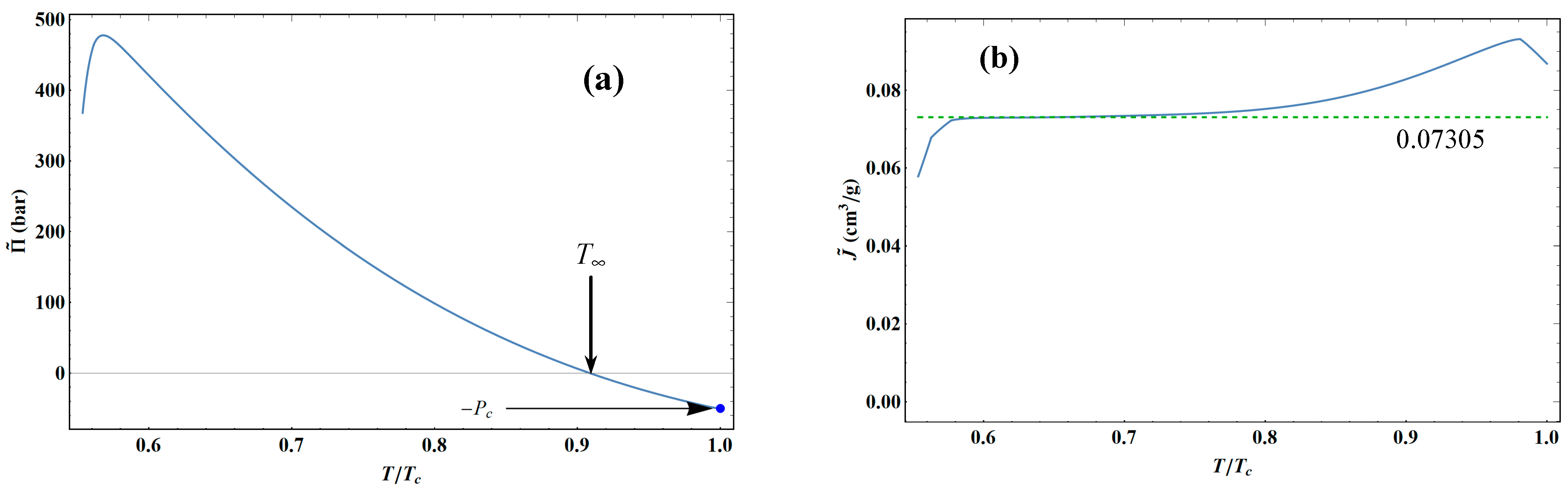
Figure 43 shows that the variations in Tait–Tammann parameters for argon are very similar to those of water (see Figure 3.4 of [
35]), except for
near the critical point, which reaches a maximum here. For many liquids, it is generally assumed that
is constant.
Figure 43b shows that this is approximately the case between 90 and 110 K for liquid argon, so the average value is
. The closeness of the variations in the Tait–Tammann parameters to those of water still implies that the Ginell parameters [
36] will have the same variations along an isotherm or isobar as those shown in Figures 3.7 and 3.8 of [
35], and consequently, the same picture of the structure of liquid argon in terms of aggregates can be drawn.
In
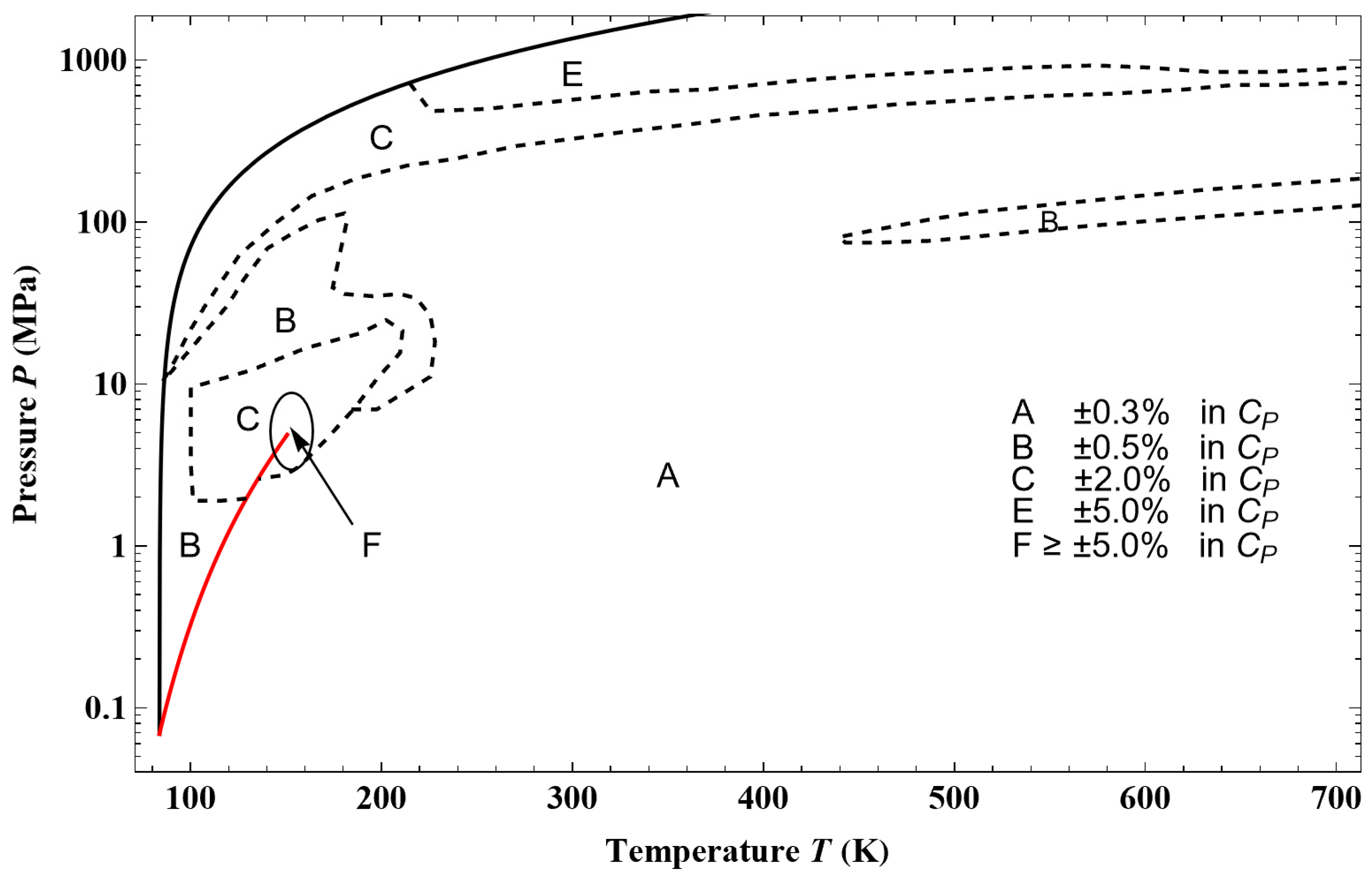
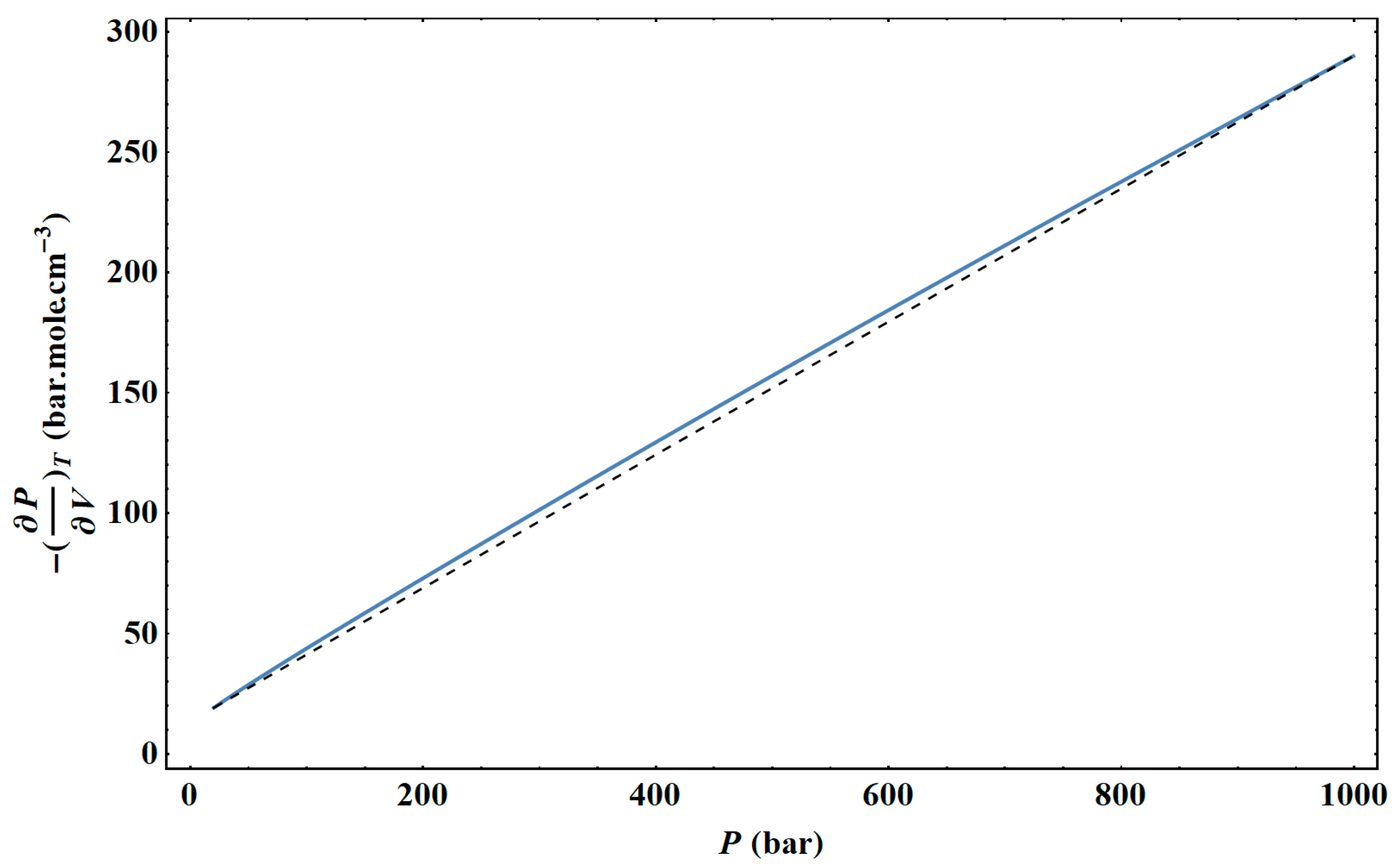
Figure 44, from an example of a given isotherm, it can be observed that the isothermal mixed elasticity modulus of liquid argon has an appreciable curvature over a pressure range of 1000 bar. Therefore, the Tait–Tammann equation over this pressure range can only be a rough approximation. If one wants to obtain a representation that fits into the tolerance diagram in
Figure 17, the pressure range must be reduced. In the case of liquid argon, the variation of the isothermal mixed elasticity modulus as a function of pressure can be considered linear for a pressure range globally below 200 bar. Above 200 bar, it was shown in Chapter 4 of [
35] that it is the adiabatic modulus of elasticity that satisfies the linearity with pressure, and therefore, a modified Tait equation must be used to describe the liquid and supercritical states of argon.
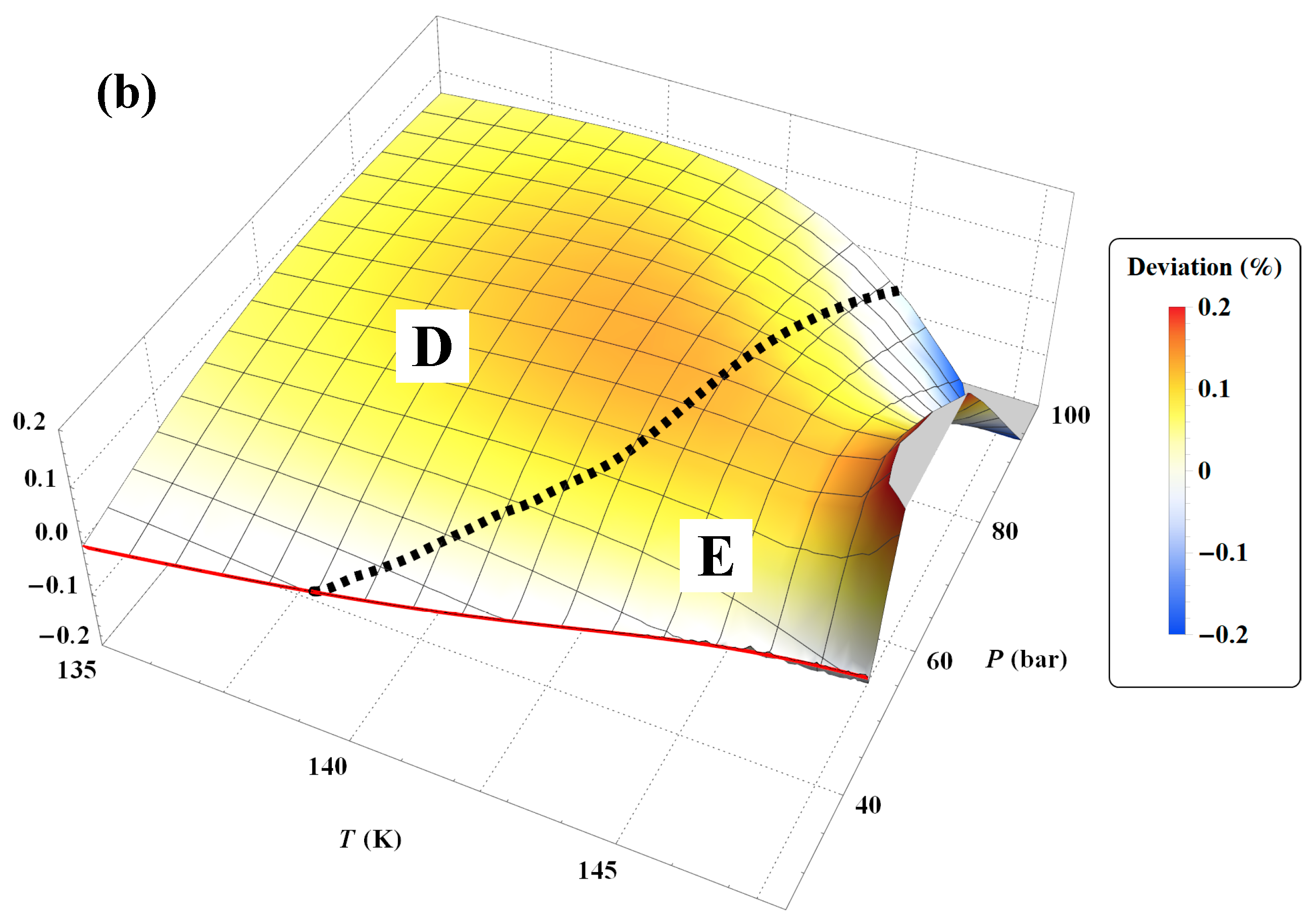
Figure 45a shows the deviation obtained between the Tait–Tammann equation of state given by Equations (71)–(73) and the present non-extensive formulation given by the inversion of Equation (45). It can be observed that the deviation essentially increases for temperatures above 140 K, so it diverges from the prescription given by the tolerance diagram in
Figure 17, which provides a tolerance of ±0.2% for subregion E.
Figure 45b shows that to achieve the tolerance of ±0.2%, the pressure range must be reduced between
Psat and 100 bar. However, the tolerance corresponding to subregion E is still slightly exceeded between 146 and 148 K.
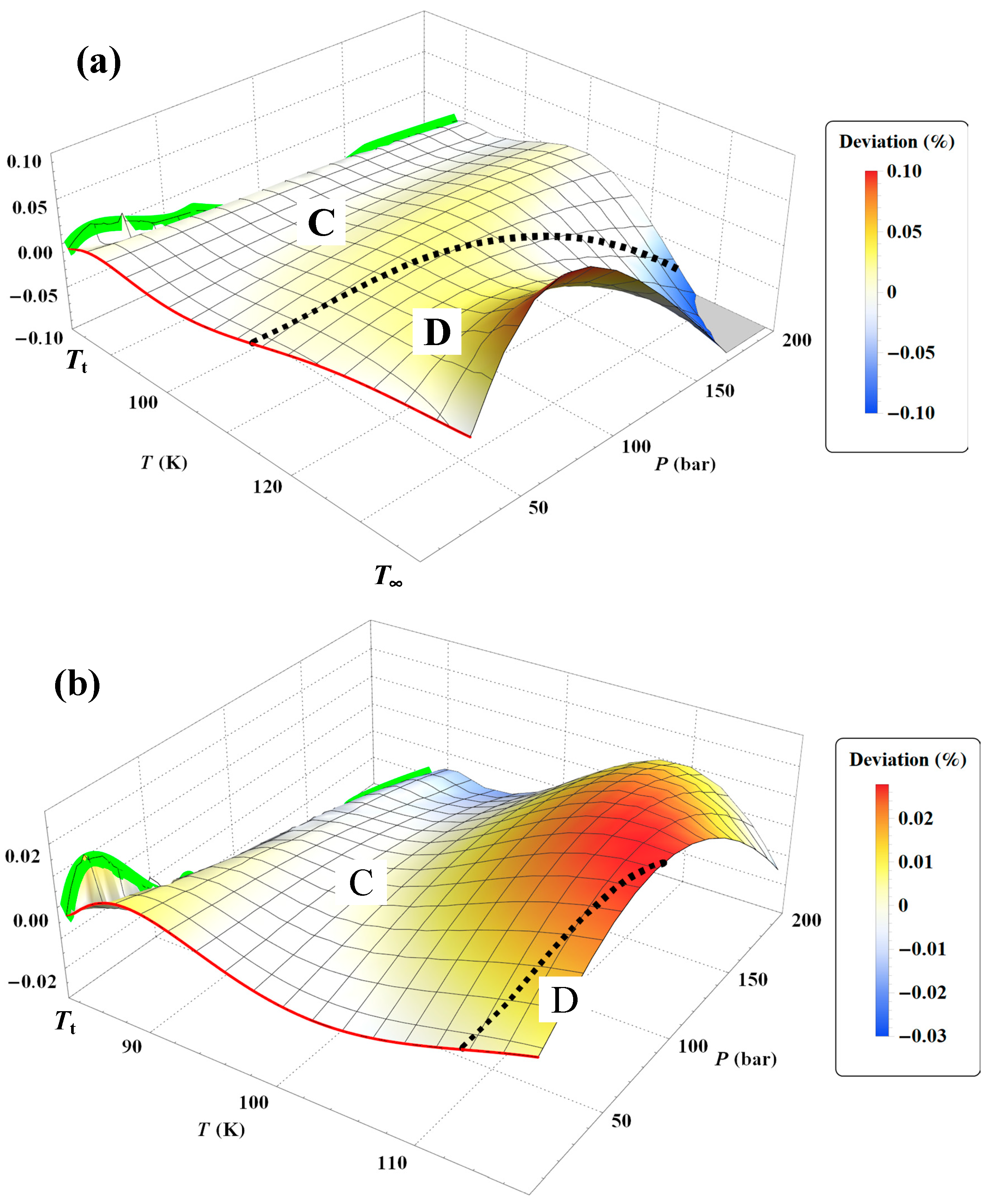
Figure 45a shows a larger negative deviation for pressures above 100 bar and temperatures above 130 K. In other words, it seems that the tolerance diagram prescription of ±0.1% for subregion D is not held at high pressures. This is confirmed by
Figure 46a, which shows that the tolerance of ±0.1% for subregion D is slightly exceeded for temperatures above 130 K and pressures above 160 bar. On the other hand,
Figure 46b shows that the tolerance diagram prescription of ±0.03% for subregion C is well achieved for the pressure range of
Psat to 200 bar. Moreover,
Figure 47 shows that the application of the Tait–Tammann equation of state up to 300 bar in subregion C leads to a deviation of ±0.05% between
Tt and 110 K and then becomes very slightly higher between 110 and 115 K for pressures above 260 bar. Even if the deviation is slightly larger than the tolerance in
Figure 17, the use of the Tait–Tammann equation of state between
Tt and 115 K can be considered a “good” approximation between
Psat and 300 bar.
Jain et al. [
37] also developed a Tait–Tammann equation to describe the specific volume of liquid argon between 90 and 148 K for a pressure range of 300 bar. It is therefore instructive to compare the evolution of the Tait–Tammann parameters with Equations (71)–(73). The form proposed by Jain et al. is such that their reference volume is no longer that of the liquid on the coexistence curve
but rather the volume corresponding to zero pressure, noted as
V0. Under this condition, the pressure
Psat is now replaced by the zero value in Equation (71). With the notations of Jain et al.,
is equivalent to
cV0, where
c is a constant and
to
B.
To cover the entire temperature range between 90 and 148 K, Jain et al. [
37] performed a piecewise determination of their equation of state as they explained:
“in two overlapping temperature ranges (i) 90 to 130 K and (ii) 127 to 148 K. […] The differences in the calculated values of V0, and B in these overlapping ranges for both liquids are less than 1 in 4000”.
Figure 48 shows the comparison between the two specific reference volumes of the Tait–Tammann equation of state for the two determinations of Jain et al. [
37] and Equations (71)–(73). It can be observed that the specific volume at zero pressure
V0 is smaller and then becomes the same as the liquid coexistence specific volume when the temperature is lower than 100 K, which is not physically acceptable. However, the saturated vapor pressure
Psat is not negligible for temperatures between 90 and 100 K; therefore, the equation of state of Jain et al. is expected to deviate strongly from the TSW model or the present non-extensive formulation in the vicinity of the saturated vapor pressure curve. However, this is a voluntary choice made by Jain et al., as they have explained below:
“At sufficiently low saturation pressures, the observed volume can be taken equal to V0, and the problem of finding a suitable value of B to represent the experimental results presents little difficulty”.
Figure 48.
Evolution of the reference volume for the Tait–Tammann equation of state as a function of temperature in the range of
Tt to 148 K: the dashed curves correspond to the two determinations of Jain et al. [
37] and the solid blue curve to
Vσl deduced from Equation (A24).
Figure 48.
Evolution of the reference volume for the Tait–Tammann equation of state as a function of temperature in the range of
Tt to 148 K: the dashed curves correspond to the two determinations of Jain et al. [
37] and the solid blue curve to
Vσl deduced from Equation (A24).
Figure 49 shows significant differences between the parameters
B and
, and
cV0 and
. However, the variations show some similarities, like the maximum of
cV0. Indeed,
Figure 49b shows that Equation (73) also has a maximum but for a slightly higher temperature than for Jain et al. [
37].
Jain et al. [
37] developed their Tait–Tammann equation of state to represent the experimental data of van Itterbeek et al. (11 isotherms that range from 90.15 to 148.25 K, TABLE I of [
38]). These experimental data were assigned by Tegeler et al. [
4] to Group 3 and therefore do not fit into the tolerance diagram of
Figure 17. Thus, the equation of state of Jain et al. is expected to represent the raw data of van Itterbeek et al. much more accurately than the non-extensive formulation of the present model or the Tait–Tammann equation of state, i.e., Equations (71)–(73).
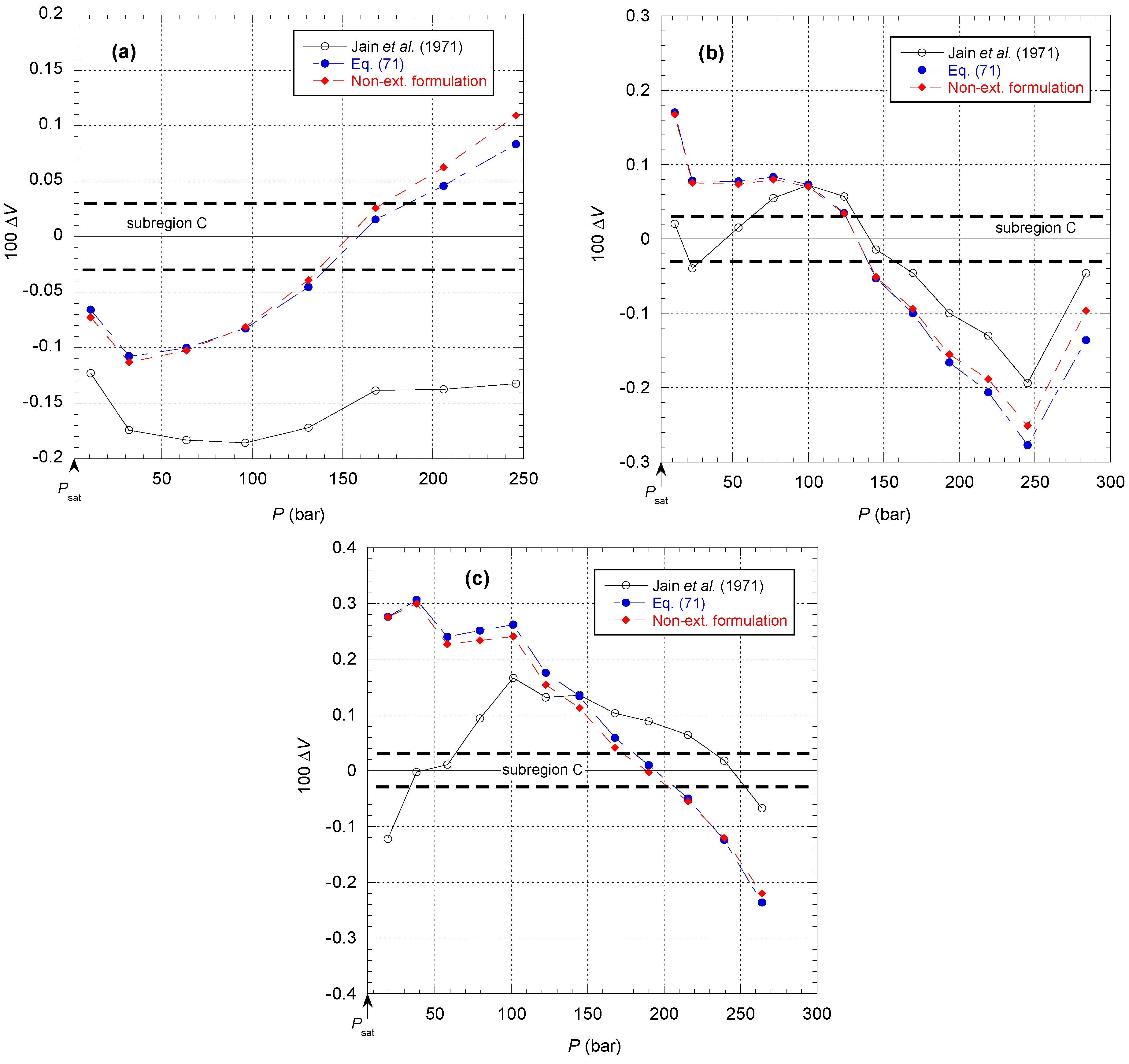
Figure 50 shows a comparison of the different models to represent the raw van Itterbeek et al. data corresponding to subregion C in
Figure 17. It can be first observed that Equation (71) and the non-extensive formulation of the present model are not much different according to the deviation in
Figure 47. It appears that the deviation of the model of Jain et al. [
37] is comparable to the other models for pressures above 100 bar, which is quite surprising. It is even more surprising to note that the model of Jain et al. appears entirely shifted by −0.15% on the lowest isotherm at 90.15 K. However, the model of Jain et al. better represents data that is close to the saturated vapor pressure curve. This is consistent with the fact that these data were not considered by Tegeler et al. to determine the liquid density on the coexistence curve.
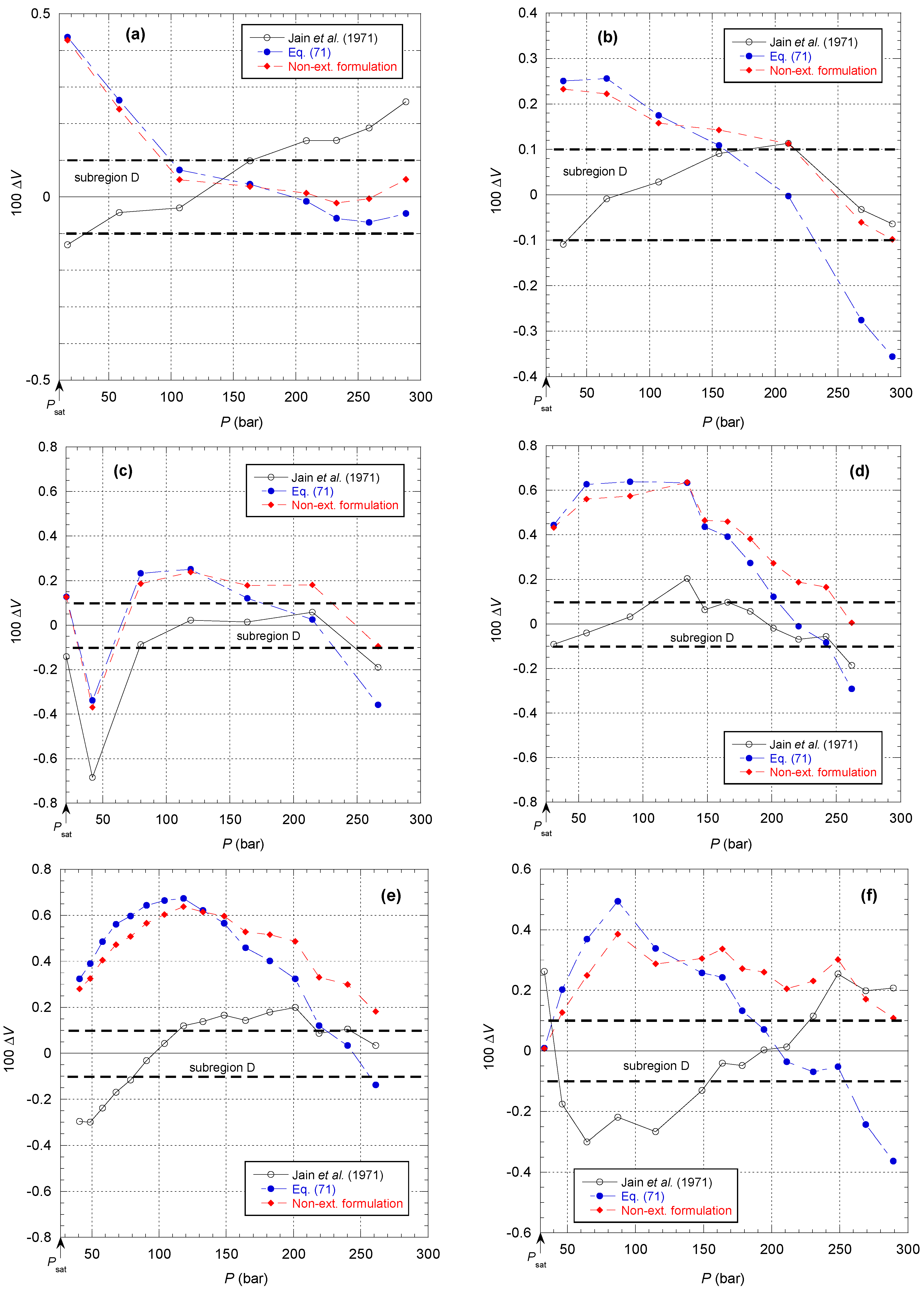
Figure 51 shows the comparison of the different models for the isotherms corresponding to subregion D in
Figure 17. It can be first observed that there is a larger deviation between the non-extensive formulation and Equation (71) beyond 150 bar, which is consistent with
Figure 46a. Then, it can be seen that the model of Jain et al. [
37] again has difficulties reproducing the data near the saturated vapor pressure curve. This can only be explained by an incorrect extrapolation to determine their function
V0(
T), if we refer to their explanation below:
“However, at high saturation pressures, both V0, and B have to be suitably chosen. The trial value of V0 is first obtained by extrapolation of the V0, against T graph from the low temperature side”.
Figure 51.
Percentage deviations of the specific volume
between the raw data of van Itterbeek et al. (TABLE I of [
38]) and the different models (i.e., Jain et al. [
37], Equation (71) and the present non-extensive formulation) for the six isotherms corresponding to subregion D in
Figure 17: (
a) 117.10 K; (
b) 127.05 K; (
c) 130.85 K; (
d) 134.40 K; (
e) 136.02 K; (
f) 138.98 K.
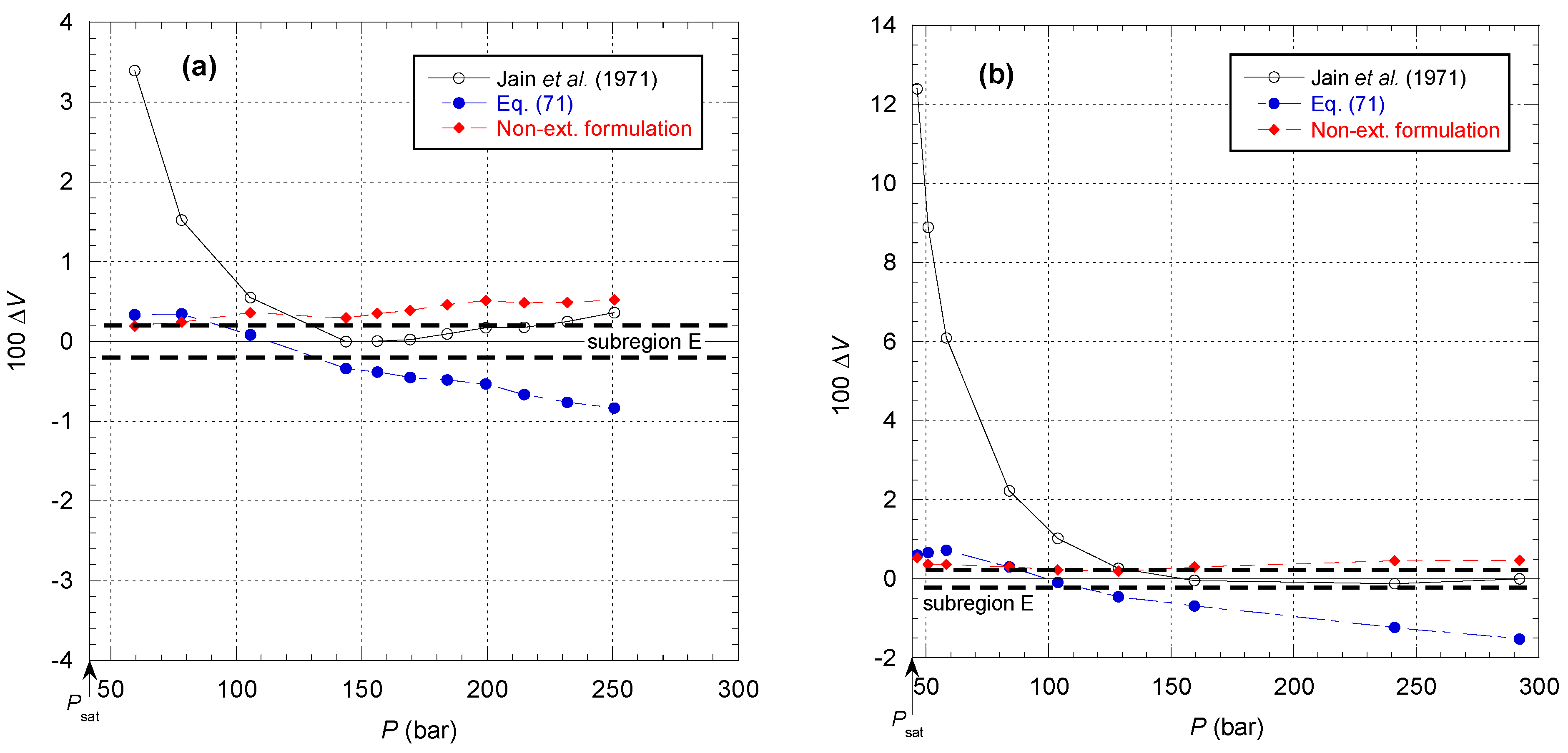
Figure 52 shows the comparison of the different models for the isotherms corresponding to subregion E in
Figure 17. It can be observed here that the deviation of the Jain et al. model from the data is greatest in the vicinity of the saturated vapor pressure curve, and the deviation is systematical in the same direction. On the other hand, this model allows data to be taken into account with the tolerance prescribed for subregion E for pressures higher than 120 bar. It can be seen that the opposite process occurs to a smaller extent for Equation (71). This is due to the curvature of the mixed elastic modulus becoming stronger and stronger, and therefore the approximation of the Tait–Tammann equation only makes sense for a smaller and smaller range of pressures. Equation (71) allows a satisfactory representation of data up to 150 bar, while the model of Jain et al. is able to reproduce data between 150 and 300 bar. The two descriptions cannot be connected except by making the Tait–Tammann parameters depend on the pressure, but under these conditions, it is preferable to use the non-extensive formulation.
In this section, it has been shown that the Tait–Tammann equation of state can be a simple alternative to describe the specific volume of liquid argon between Tt and 148 K, for pressures varying between Psat and 300 bar in subregion C, then between Psat and 200 bar in subregion D, and finally between Psat and 100 bar for subregion E. These pressure ranges are sufficient for a very large number of applications.
7. Conclusions
A new equation of state for argon was developed, which can be written in the form of a fundamental equation explicit in the reduced Helmholtz free energy. This equation was derived from the measured quantities
CV(
ρ,
T) and
P(
ρ,
T). It is valid for the whole fluid region (single-phase and coexistence states) from the melting line to 2300 K and for pressures up to 50 GPa. The formulation is based on data from NIST (or equivalently on the calculated values from the TSW model) and calculated values from the model of Ronchi [
7].
This new approach, using mainly power laws with density-dependent exponents, involves much fewer coefficients than the TSW model and, more importantly, eliminates the very small oscillations introduced by a polynomial description. This leads to a more physical description of the thermodynamic properties. On the other hand, the reduction in the number of terms and parameters does not modify the uncertainties of the calculated data in an appreciable way (as shown in the different diagrams of tolerance). However, in an unexpected way, the present approach, which generates more regular and monotonous expressions, raises greater difficulty for the reversal of certain equations of state due to the highly nonlinear behavior of these expressions.
The new equation of state also shows more physical behavior along isochors when
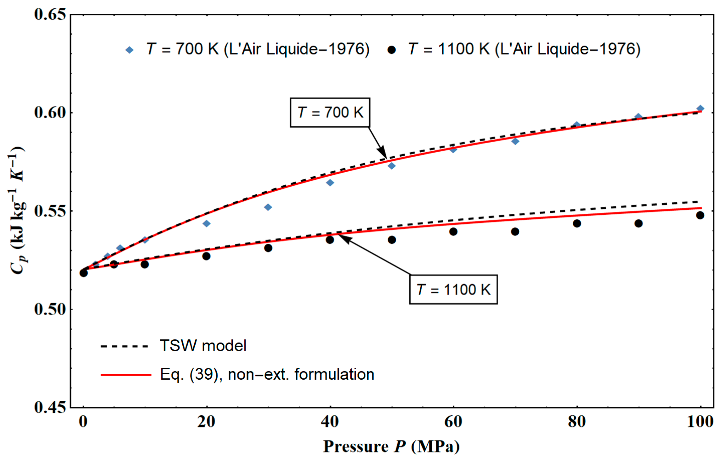
T tends to zero for basic properties, such as the isochoric heat capacity and the compressibility factor. It also shows a more reasonable behavior for the crossing of the coexistence phase. However, it does not correctly describe the properties in the vicinity of the critical point, in the same way as the TSW model does not properly describe the properties in the vicinity of the critical point, with the exception of the saturation curve. However, variations in the isochoric heat capacity in the coexistence phase with the present model show peaks that are qualitatively in agreement with experimental observations, unlike the TSW model, which produces unphysical variations. Comparison of the present model with the data of L’Air Liquide [
5], which had not previously been taken into account, shows that this model is consistent with data up to 1100 K and 100 MPa, which allows, regardless of the data of Ronchi [
7], the range of NIST data to be extended [
6].
In
Section 6 and
Appendix C, simple expressions are also provided to describe the specific volume of the liquid states of argon between
Tt and 148 K in the form of a Tait–Tammann equation of state and some properties of the liquid–vapor coexistence curve. These approximate formulas can advantageously replace the complex, non-extensive formulation of the present model for a large number of applications.
The non-extensive approach developed here shows that metastable states are, by construction, included as an extension of single-phase isochoric heat capacity modeling. As CV data are generally known for the vast majority of fluids, this new approach can be easily extended to all of them.


