Abstract
This study introduces a novel approach using 3D Physics-Informed Neural Networks (PINNs) for simulating blood flow in coronary arteries, integrating deep learning with fundamental physics principles. By merging physics-driven models with clinical datasets, our methodology accurately predicts fractional flow reserve (FFR), addressing challenges in noninvasive measurements. Validation against CFD simulations and invasive FFR methods demonstrates the model’s accuracy and efficiency. The mean value error compared to invasive FFR was approximately 1.2% for CT209, 2.3% for CHN13, and 2.8% for artery CHN03. Compared to traditional 3D methods that struggle with boundary conditions, our 3D PINN approach provides a flexible, efficient, and physiologically sound solution. These results suggest that the 3D PINN approach yields reasonably accurate outcomes, positioning it as a reliable tool for diagnosing coronary artery conditions and advancing cardiovascular simulations.
1. Introduction
Coronary artery disease (CAD) remains a significant global health challenge [1], emphasizing the need for accurate computational models to understand its underlying pathophysiology and devise effective interventions. Computational fluid dynamics (CFD) simulations play a crucial role in elucidating blood flow behavior in coronary arteries, aiding in diagnosis and treatment planning. However, traditional CFD approaches are often computationally intensive, limiting their clinical applicability. Recent advancements in deep learning, particularly physics-informed neural networks (PINNs), offer promising opportunities to expedite and enhance coronary artery flow modeling. In the next work, a review of the relevant literature will synthesize the recent literature focusing on the application of 3D PINN simulations in coronary artery trees, covering methodologies, applications, and future directions.
The 3D PINN method offers a novel, non-invasive approach for stenosis diagnosis, bypassing the limitations of invasive techniques such as coronary angiography. It minimizes patient invasiveness, reduces costs, and enhances safety by lowering procedural risks.
Recent studies have highlighted the potential of PINNs to transform computational cardiovascular medicine and investigated the integration of deep learning techniques, specifically PINNs, with traditional CFD and fluid–structure interaction (FSI) methods to accelerate coronary artery flow simulations. Taebi (2022) provided a comprehensive review of deep learning applications in computational hemodynamics, highlighting the potential of PINNs to reduce the computational burden of patient-specific simulations [2]. Moser et al. (2023) compared various neural network architectures for physics-informed flow modeling, emphasizing the efficacy of more sophisticated models such as the deep Galerkin method [3]. Arzani et al. (2021) demonstrated the effectiveness of PINNs in quantifying near-wall blood flow from sparse data, addressing challenges encountered in patient-specific CFD models [4]. These studies underscore the versatility of PINNs in integrating physiological principles with data-driven approaches to improve coronary artery flow predictions.
In recent years, data-driven approaches have emerged as powerful tools for enhancing our understanding and management of CAD. This section describes the application of data-driven methods, such as machine learning and artificial intelligence, in CAD research and clinical practice.
Machine learning techniques have gained popularity in CAD risk prediction and diagnosis. Researchers have harnessed the vast amount of patient data available to develop predictive models. These models consider a multitude of factors, such as medical history, genetic information, and lifestyle, to assess an individual’s CAD risk.
Two noteworthy studies by Abdar et al. (2019) and J. I. Z. Chen and P (2021) presented innovative approaches for predicting CAD using machine learning methods. The first study proposed a pooled area curve (PUC) algorithm for early CAD prediction, focusing on identifying variations in medical imaging to aid in preventive measures. In contrast, the second study describes an optimized machine learning methodology that leverages genetic algorithms and particle swarm optimization to achieve high accuracy in CAD detection. Both studies have contributed valuable insights to improving CAD diagnosis and prognosis [5,6].
Several studies have investigated the effectiveness of finite element analysis (FEA) and physics-informed neural networks (PINNs) in handling partial differential equations (PDEs) across various domains, particularly in fluid flow scenarios. Recent research has explored the fusion of AI, machine learning (ML), and computational fluid dynamics (CFD) to better understand hemodynamics and biomechanics in cardiovascular diseases, emphasizing the importance of precise prediction and diagnosis.
X. Li et al. (2022) underscored the collaboration between artificial intelligence (AI) and biomechanics modeling in predicting cardiovascular diseases (CVDs) [7]. Their study highlighted machine learning’s role in directly forecasting CVD through risk factors and medical imaging findings, as well as its utility in hemodynamics with vascular geometries. Zhang et al. (2023) focused on the application of PINNs for 4D hemodynamic prediction, demonstrating their effectiveness in generating flow field datasets for personalized models and enabling accurate space–time behavior forecasts [8]. Arzani et al. (2022) discussed the challenges and opportunities of using ML for cardiovascular biomechanics modeling, emphasizing the strategic integration of ML to augment traditional physics-based modelling [9]. Moradi et al. (2023) emphasized the role of machine learning in enhancing computational fluid dynamics, blood flow imaging, and wearable sensing technologies, offering promising solutions to address computational cost and data analysis constraints [10].
Recent studies have also explored the specific application of ML and PINN in the context of coronary artery disease. Farajtabar et al. (2023) introduced a novel deep neural network framework for predicting blood flow behavior in patient-specific coronary arteries with abnormalities, achieving high accuracy in pressure and velocity magnitude predictions [11]. Taebi (2022) investigated the integration of deep learning with CFD, particularly in solving hemodynamic problems in the aorta and cerebral arteries, anticipating a shift in computational medical decisions [2]. Additionally, Sarabian et al. (2022) developed a physics-informed deep learning framework for brain hemodynamic predictions, showing its potential for accurately estimating cerebral hemodynamic variables [12]. Isaev et al. (2024) utilized PINNs to estimate blood flow parameters in post-Fontan four-vessel junctions, demonstrating the applicability of PINNs in complex cardiovascular anatomies [13].
Several studies have underscored the importance of fluid–structure interaction (FSI) analysis in comprehending hemodynamics in specific arteries. Lee et al. (2012) conducted a thorough numerical investigation of carotid artery hemodynamics using FSI, highlighting the significant influence of geometric factors and flow conditions on carotid artery hemodynamic characteristics. They extended this analysis to examine a model for atherosclerotic carotid artery bifurcation, identifying key stress factors contributing to artery wall dissection [14]. Nolte and Bertoglio (2022) provided a comprehensive review of inverse problems in blood flow modeling, focusing on formulating and numerically solving inverse problems using clinical data, primarily medical images, for personalized spatially distributed models of the vasculature [15]. Additionally, Ma (2023) proposed innovative strategies combining magnetic resonance imaging (MRI), CFD, and PINN for the quantitative study of hemodynamics, emphasizing their potential in precision medicine and personalized medical therapy [16].
Aligned with these findings, Du et al. (2023) introduced a novel method for pressure estimation based on physics-informed neural networks, offering an effective approach for predicting intravascular pressure in aortic arch models, with implications for diagnosing cardiovascular diseases [17]. In the study by Alzhanov et al. (2023), a novel physiologically based algorithm (PBA) was developed for computing fractional flow reserve (FFR) in coronary artery trees (CATs) using computational fluid dynamics (CFD). The PBA extends Murray’s law and incorporates additional inlet conditions, prescribed iteratively. Implemented in OpenFOAM v1912, this algorithm was tested and validated using 3D models of CATs created from CT scans and computational meshes. The validation involved comparing the PBA results with invasive coronary angiographic (ICA) data [18].
As we delve deeper into the realm of hybrid physics/data-driven and multiscale/multiphysics methods for CAD research, it is crucial to acknowledge the challenges that researchers face and chart a course for future advancements. This section discusses the prominent challenges and outlines potential directions for CAD simulation research.
In summary, the reviewed literature underscores the growing integration of AI, ML, CFD, and FSI methods in cardiovascular disease research, and particularly in the development of hybrid physics/data-driven and multiscale/multiphysics simulation methods for patient-specific analysis and diagnosis of coronary artery disease. These integrated approaches demonstrate promising potential in improving the accuracy and efficiency of cardiovascular disease prediction and treatment, potentially transforming cardiovascular biomechanics research and clinical practice.
Three-dimensional Physics-Informed Neural Networks (PINNs) differ from their 2D and 1D counterparts in their ability to model complex three-dimensional (3D) physical systems, such as flow in arteries, aerodynamics around complex geometries, or heat transfer in intricate 3D structures. While 2D PINNs are limited to two-dimensional systems and 1D PINNs to one-dimensional systems, 3D PINNs extend the capability to capture spatial variations and boundary interactions in three dimensions, offering more accurate and detailed simulations of real-world phenomena with higher complexity and fidelity.
The main objective of this study is to develop and validate a novel, non-invasive approach for diagnosing coronary artery stenosis using 3D Physics-Informed Neural Networks (PINNs). This method aims to overcome the limitations of invasive techniques such as coronary angiography by minimizing patient invasiveness, reducing costs, and enhancing safety by lowering procedural risks.
Our methodology integrates 3D PINNs without providing customized outflow boundary conditions, ensuring precise diagnostic accuracy without the need for extensive empirical data. By incorporating synthetic data, our approach closely aligns with real-world physiological phenomena. The 3D PINN simulations are designed to accelerate and refine coronary artery flow modeling, offering valuable insights into hemodynamic and disease mechanisms. The study adheres to ethical standards with Institutional Review Board (IREC) approval, ensuring patient confidentiality and ethical compliance.
2. Mathematical Formulations and Numerical Methods
Traditional Computational Fluid Dynamics (CFD) methods, such as the finite element method (FEM), finite volume method (FVM), and finite difference method (FDM), are used to solve Navier–Stokes equations by discretizing the computational domain and iteratively solving the equations. However, applying these methods to arterial blood flow presents significant challenges due to complex geometries, dynamic and nonlinear boundary conditions, and high computational costs. The intricate branching of arterial networks, the pulsatile nature of blood flow, and the elastic properties of arterial walls make accurate discretization and boundary condition application difficult. Additionally, traditional CFD methods require substantial computational resources and are highly sensitive to initial and boundary conditions, leading to potential errors. These challenges highlight the need for innovative approaches like the 3D Physics-Informed Neural Network (PINN) method, which integrates deep learning with fundamental physics principles for more efficient and accurate simulations.
2.1. Governing Equations for Hemodynamic Flow
The dynamic behavior of a fluid is generally described by the Navier–Stokes and continuity equations.
Assumptions:
Flow Type: Unsteady flow.
Compressibility: Incompressible flow.
Fluid Nature: Newtonian fluid.
Fully developed laminar flow.
Flow in a patient-specific artery.
Physical Properties: constant physical properties of the fluid viscosity of 0.0035 Ns/m2 and a density of 1056 kg/m3.
2.1.1. Continuity Equation
For incompressible flow, the continuity equation is expressed as
where u is the velocity vector.
2.1.2. Equation of Motion (Navier–Stokes Equation)
The Navier–Stokes equation for incompressible, Newtonian fluid flow is given by
where the definitions are as follows:
- u is the velocity vector;
- t is time;
- ρ is the fluid density (constant);
- p is the pressure;
- ν is the kinematic viscosity (constant);
- f represents body forces (e.g., gravity).
2.1.3. Reynolds Number in Artery Flow
The Reynolds number is a crucial dimensionless parameter in characterizing blood flow in arteries. For laminar flow in arteries, it can be expressed as:
where the definitions are as follows:
- ρ is the density of blood;
- uavg is the average flow velocity derived from the Hagen–Poiseuille equation;
- D is the diameter of the artery;
- μ is the dynamic viscosity of blood.
By evaluating the Reynolds number, one can predict the flow regime and ensure that the assumptions of laminar flow are valid.
2.1.4. Significance of the Reynolds Number
For laminar flow, Re < 2000 (typically less than 1000 in small arteries due to their smaller diameter and slower flow rate).
For transitional flow, 2000 ≤ Re ≤ 4000.
For turbulent flow, Re > 4000.
In arteries, because the Reynolds number often remains below the critical threshold (2000), the flow is typically laminar under normal physiological conditions. However, in certain pathological conditions or in larger arteries with higher flow rates, the Reynolds number can approach or exceed the critical value, leading to turbulence.
2.2. Physics-Informed Neural Networks
Physics-informed neural networks, commonly known as PINNs, offer a novel approach, leveraging recent advancements in deep learning to infer solutions and parameters. The concept of PINNs was proposed by Raissi et al. (2019), wherein the partial differential equation (PDE) governing the physical system is integrated into the loss function of a neural network [19,20]. This inclusion of an additional constraint results in a solution that progressively converges to one consistent with the fundamental laws of physics. PINNs have the capability to directly produce the solution of a physical system based solely on the underlying PDE, along with initial and boundary conditions, eliminating the necessity for supplementary data such as measurement data. In essence, a physical system can be characterized by this set of equations.
In this context, [·] represents a nonlinear differential operator acting on the solution u(x), where Ω signifies the geometry and [·] characterizes the boundary conditions of the geometry on the boundary ∂Ω. This paper focuses on transient systems, with the need for initial conditions. Following the approach introduced by Raissi et al., 2019, we approximate the solution u(x) using a deep neural network denoted as (x; ), where represents the trainable parameters (i.e., weights and biases) [20].
In a standard fully connected architecture, neurons in adjacent layers are connected, whereas neurons inside a single layer are not linked. The network output of a neural network (NN) with n layers takes the following form.
where is the i-th layer. and are the weights and biases of the i-th layer, x is the network’s input, and are the activation functions used throughout this paper. The represents the set of trainable parameters .
2.3. Loss Function: Accounting for All Constraints
In the preceding sections, we outlined the process of formulating the separate components of the loss function, encompassing measurements, physical constraints, and continuity which the model needs to adhere to. In this section, we will elucidate how to integrate these individual components to establish the comprehensive structure of the loss function. We will also provide descriptive examples to interpret the procedure, which was obtained from Raissi et al. (2019) [20].
The overall loss function comprises multiple components: (a) , a loss term derived from the residuals of the PDE; (b) , a loss term determined by the boundary conditions; and (c) , a loss term calculated based on potentially available sparse measurement data.
Equation (9) represents the mean squared residuals of the PDE assessed at randomly chosen points within the geometric space. Similarly, Equation (10) assesses the boundary loss by considering randomly selected points along the boundary of the geometry. In Equation (11), the points denote the locations where the solution u may be available or measured. The data loss term in Equation (8) is enclosed in brackets, since it could incorporate available measurement data into the PINN training process, although it was utilized in this study. The weighting parameters (, , ) regulate the significance of the loss terms. The objective of PINN training is to determine the optimal set of network parameters q using various optimization algorithms (e.g., Adam by [21]) to minimize the loss function L.
3. Model Setup and Boundary Conditions
While the literature on physics-informed neural networks (PINN) presents a variety of network architectures, there is a prevailing tendency toward larger networks [2]. The problem solution is parameterized through three distinct neural networks, each dedicated to a specific residual boundary condition coronary artery tree. Given the intricacies of our 3D flow simulations, we decided to adopt a network structure consisting of 10 layers, each comprising 256 neurons, a configuration inspired by prior PINN studies on fluid dynamics [22]. To ensure consistency, we maintained the same network size, activation functions (swish with parameter b = 1) [23], exponentially decaying learning rates (initialized at 0.0001 with a decay rate of 0.97 over 10,000 steps), and Adam and L-BFGS optimizers across all PINN architectures utilized in this research. Additionally, equal weighting for the loss terms in Equation (8) was applied for uniformity in comparison. This architectural configuration has the capacity to effectively capture intricate features inherent in propagating waveforms.
The PINN solver used a total of 1 × 10⁵ randomly sampled spatial points per epoch during the training process. A batch size of 10,000 was used, i.e., 1 × 10⁴ points were employed in each training iteration.
In this study, two types of PINN simulations were conducted: one with training and one without training data. The main boundary conditions for each are presented in Table 1 and Table 2. The key differences between these simulations lie not only in the training data but also in the boundary conditions. The PINN with training data uses both pulsatile velocity and pressure with no outlet conditions, while the PINN without training data uses only the average static pressure from Table 3 with zero pressure outlet conditions. The training data for the first case were derived from the transient results in CFD PBA methodology [18]. Additionally, in the first case, each of the three arteries was trained and run separately, whereas in the second case, the model was trained only based on physics of the Navier–Stokes equation on the CHN13 model, enabling it to generate results for other arteries without additional training for other geometries separately.

Table 1.
Boundary conditions used in the PINN with training data.
Table 2.
Boundary conditions used in the PINN without training data.
Table 3.
Experimentally obtained input parameters for simulation of CHN13.
In our CFD model of arterial blood flow, the following boundary conditions are employed: a pulsatile inlet velocity and pressure to represent the time-varying nature of blood flow driven by the cardiac cycle, no specified outlet condition assuming a sufficiently large computational domain, and a no-slip condition at the arterial walls reflecting the zero velocity of blood at the wall ((u) = 0). Additionally, a Navier–Stokes residual boundary condition is applied at internal boundaries or interfaces within the computational domain to manage and minimize the residuals of the Navier–Stokes equations, stabilizing the numerical solution and ensuring continuity and momentum balance. This approach is crucial for achieving an accurate and stable representation of the fluid dynamics within the artery. The boundary conditions are shown in Table 1 and Table 2.
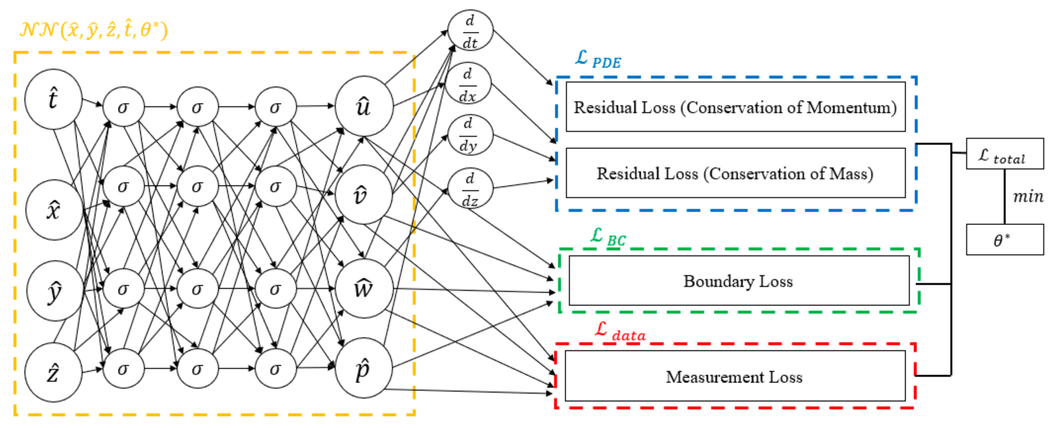
All calculations (PINN training) were performed on a workstation with a Xeon(R) Gold 5220, NVIDIA Tesla T4, and 64 GB of RAM (NVIDIA, Santa Clara, CA, USA). Schematic illustration of the proposed algorithm are shown in Figure 1.
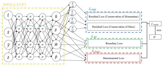
Figure 1.
The diagram delineates the distinct components of the loss function. The blue box signifies the portion related to residual losses, the green box corresponds to boundary losses, and the red box represents measurement loss. The amalgamation of these components constitutes the comprehensive loss function, where the tuning of neural network parameters is achieved through minimization.
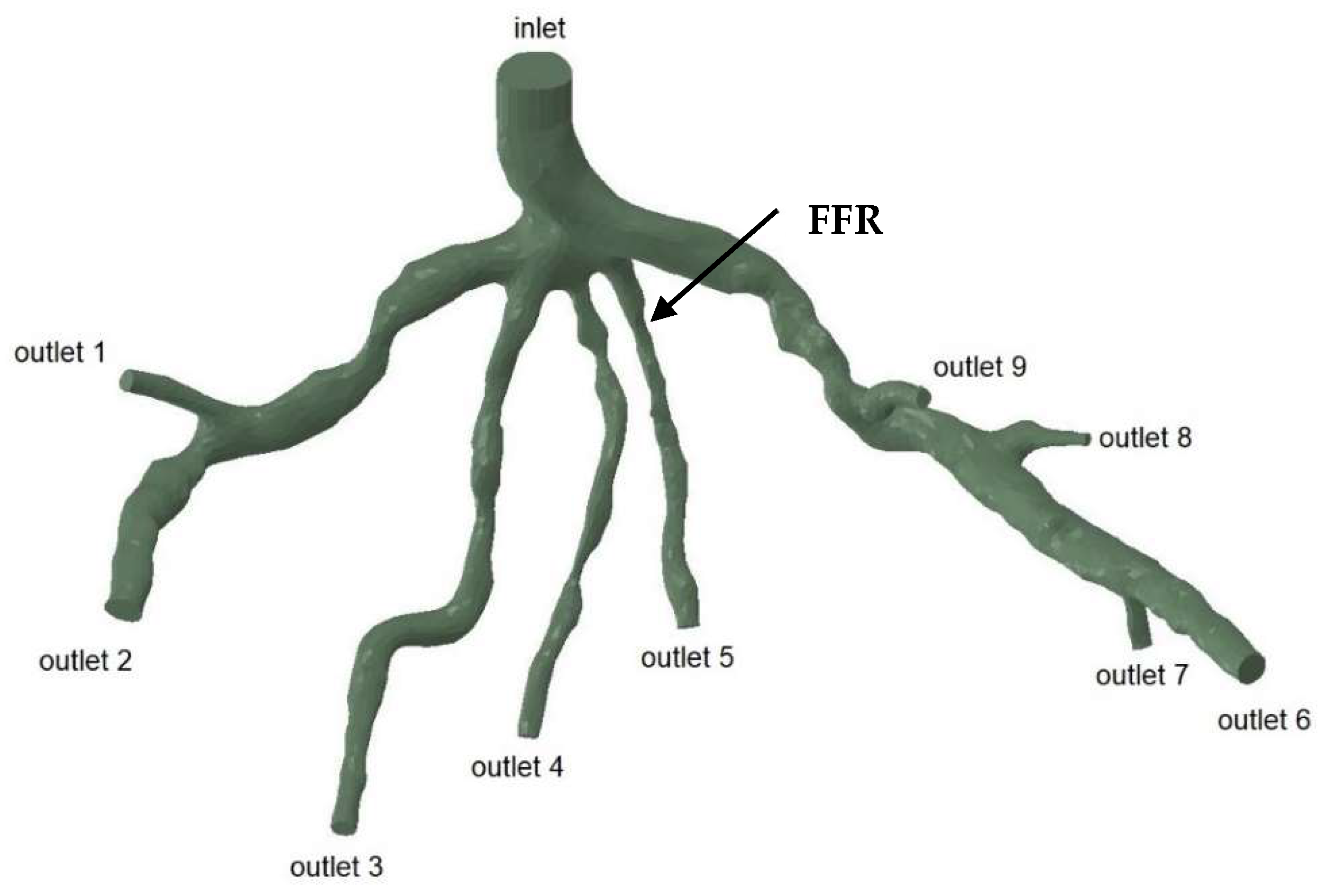
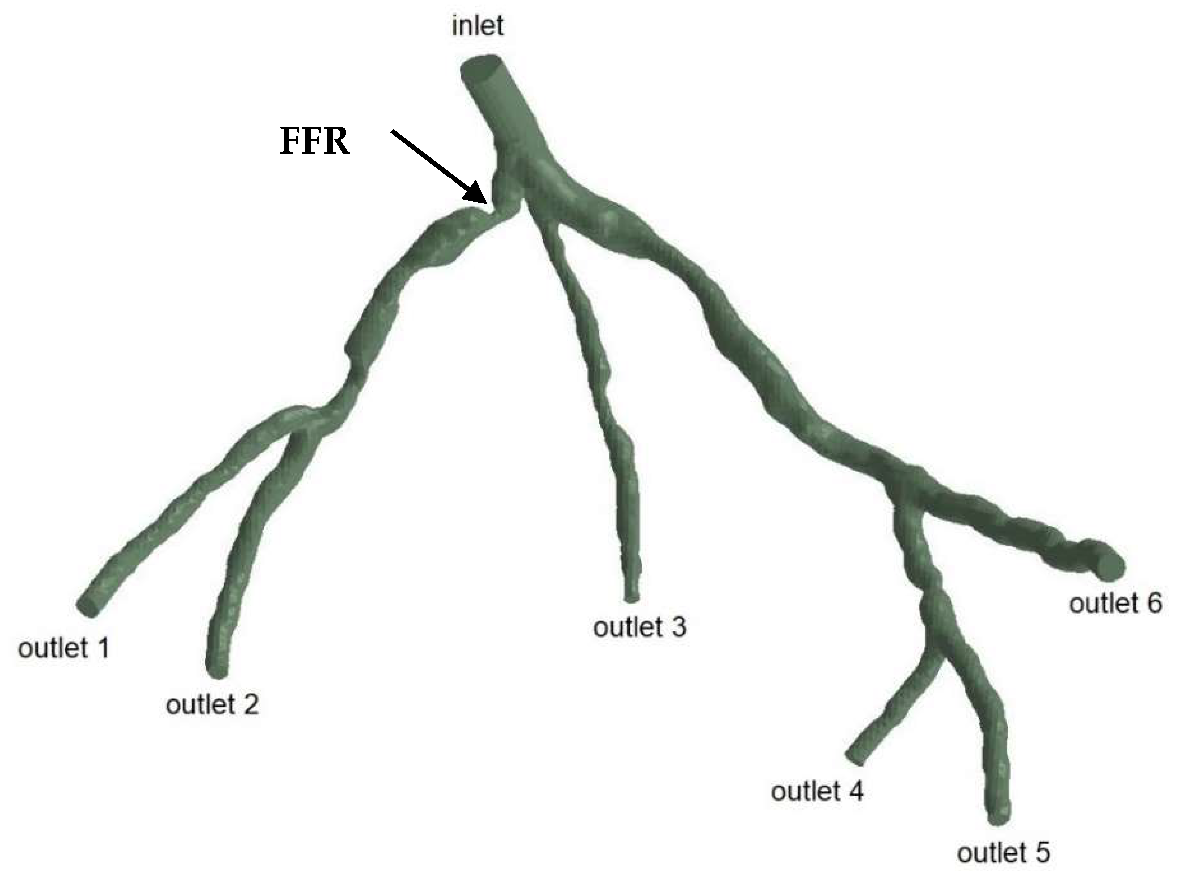
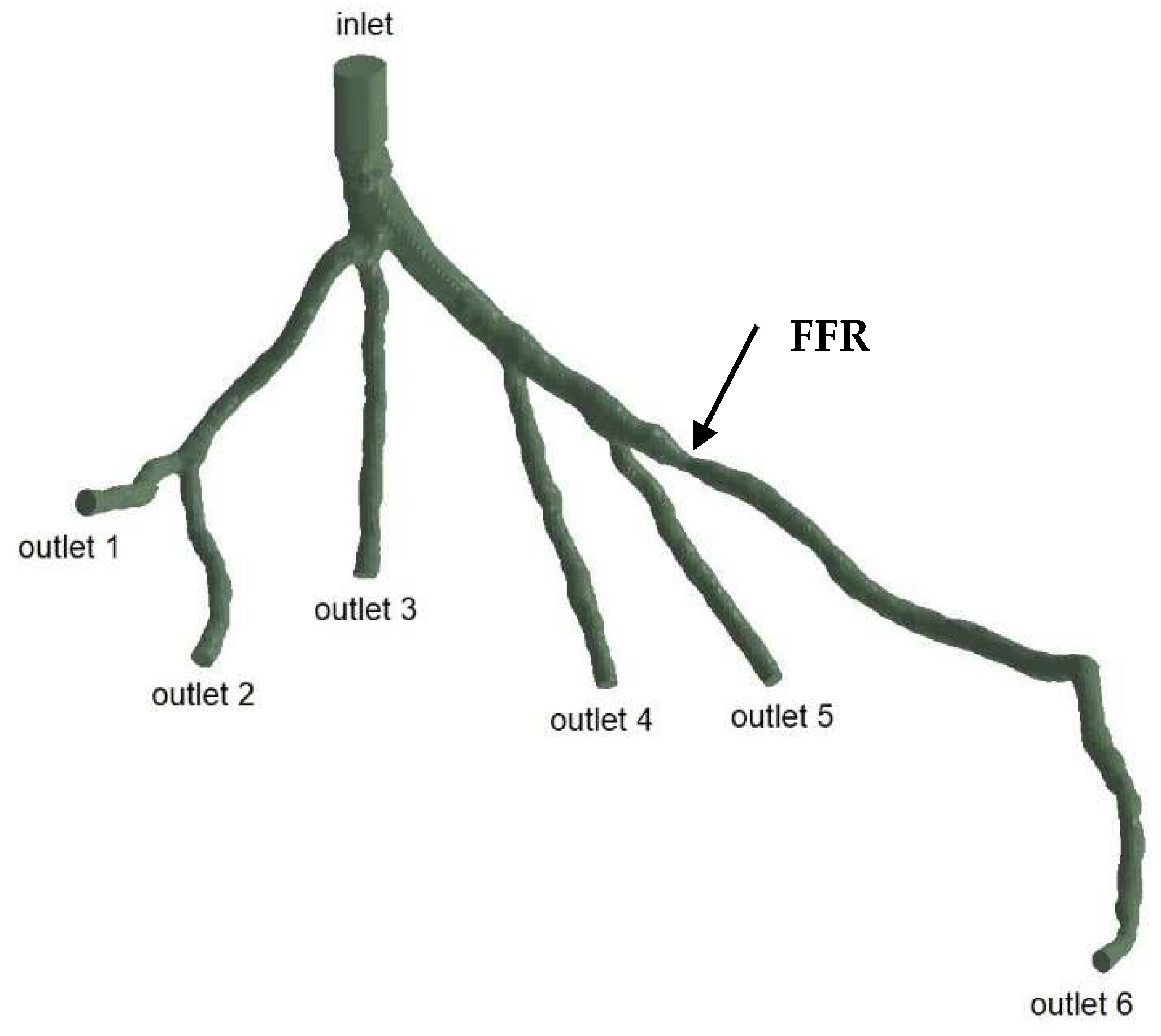
The geometries and outlets of CT209, CHN13, and CHN03 are presented in Figure 2, Figure 3 and Figure 4, respectively.

Figure 2.
Geometry and inlet/outlets of the CT209 model.
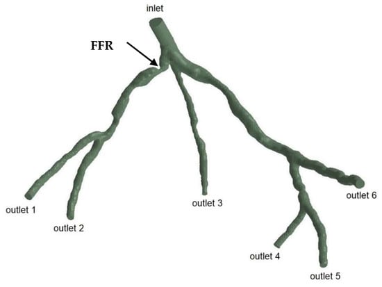
Figure 3.
Geometry and inlet/outlets of the CHN13 model.

Figure 4.
Geometry and inlet/outlets of the CHN03 model.
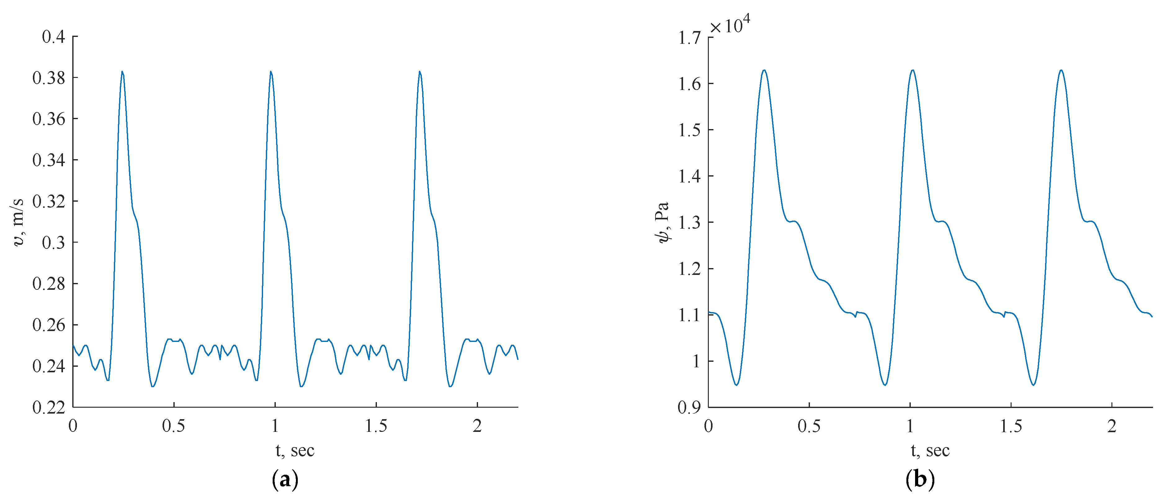
The transient inlet values are shown in Figure 5.
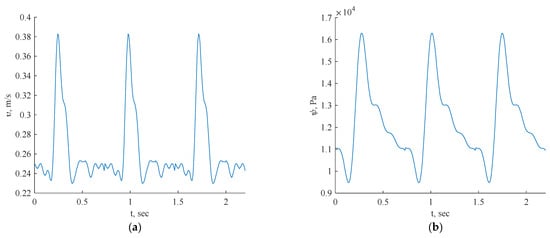
Figure 5.
Inlet boundary conditions: transient velocity (a) and pressure (b) waveforms of coronary blood flow.
For this investigation, uniform fluid properties and blood models were employed, featuring a Newtonian dynamic viscosity of 0.0035 Ns/m2 and a density of 1056 kg/m3 [24]. The simulations were conducted with velocity/pressure inlets as boundary conditions, defining the blood flow as laminar fluid flow. The inlet data for each artery specified the consistent use of three cycles in all the simulations.
In Figure 5, the pulsatile velocity vector v = [u(x), v(x), w(x)] represents the velocity magnitude, while p = p(x) denotes the pressure field. The inflow was set to be perpendicular to the inlet plane, with boundary conditions including a no-slip condition on the geometry walls (u, v, w = 0) and no pressure condition at the outlet. The blood was modeled as a laminar fluid, dependent on the geometry.
The FFR is computed using a formula as previously carried out in the CFD PBA method [18] (12).
4. Results and Discussion
4.1. Three-Dimensional Artery Tree Validation with Training Data
The proposed methodology will be tested in a scenario where we consider two inlet velocities and pressures without applying outlet boundary conditions. In this scenario, we examine prototypes of arterial networks depicted in Figure 2, Figure 3 and Figure 4. The key innovation lies in the fact that we use training data generated from the CFD PBA method [18] and without outlet boundary conditions, and the model will be trained based on both physics equations using DeepXDE (https://deepxde.readthedocs.io/en/latest/) library and training data, code added in Appendix A. This software can solve forward problems given initial and boundary conditions, and supports complex-geometry domains through the technique of constructing solid geometry. The authors noted from their experience that for smooth partial differential equation (PDE) solutions, L-BFGS tends to converge in fewer iterations than does Adam. This is attributed to L-BFGS’s utilization of second-order derivatives of the loss function, while Adam relies solely on first-order derivatives [25].
Additionally, a comprehensive systematic study will be conducted to assess the accuracy and robustness of the proposed method. The implementation of the proposed algorithms utilizes TensorFlow v1.10.
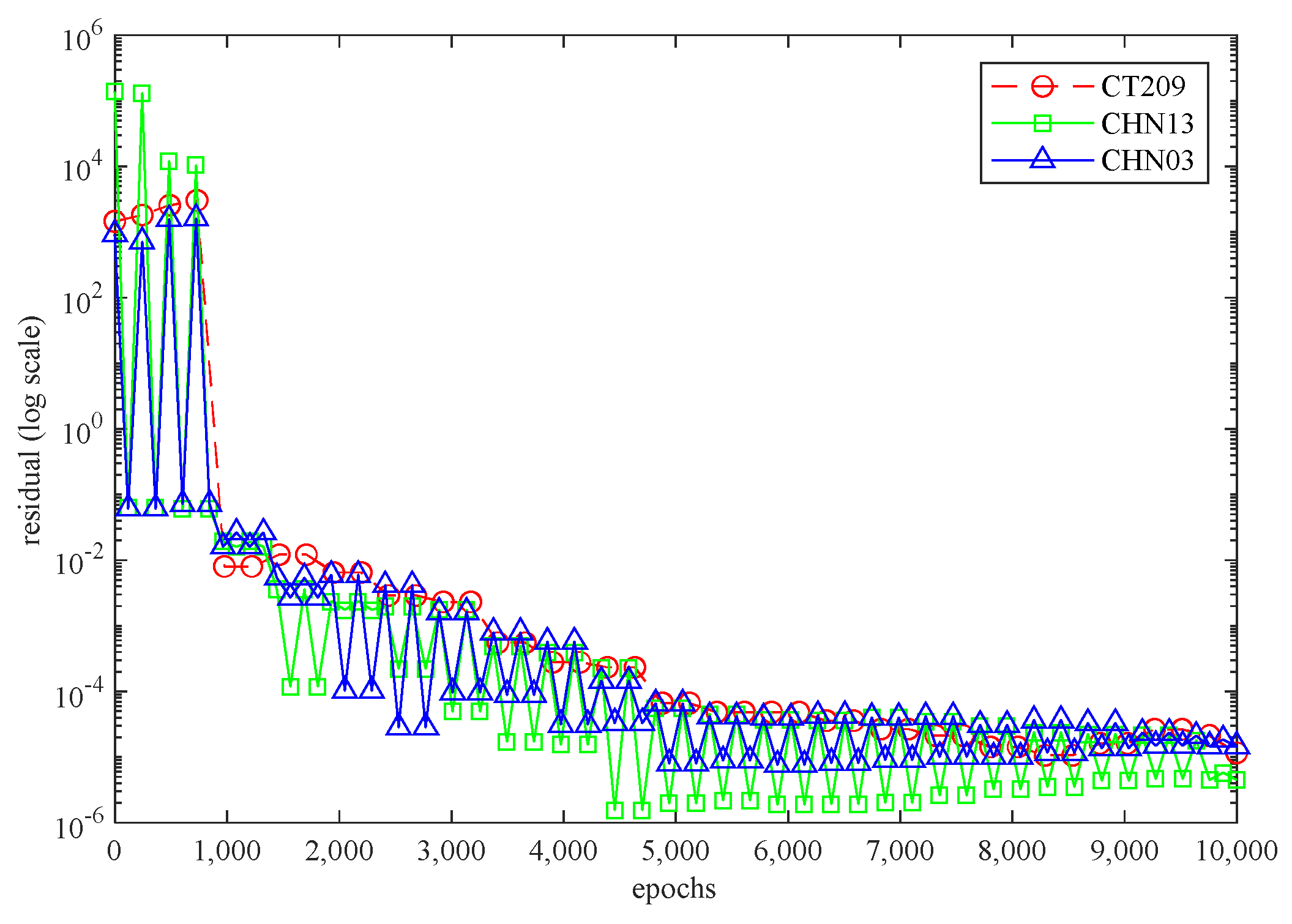
Figure 6 illustrates the 3D PINN residual history for each artery while the neural network is running. In all three scenarios, the residual values surpassed 10−4 and were within the range of 10−4 to 10−6. This suggests that all three cases exhibit satisfactory convergence, indicating accurate calculations by the code.
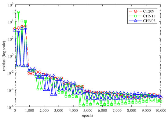
Figure 6.
The 3D PINN residual history for each artery.
4.2. Fractional Flow Reserve (FFR)
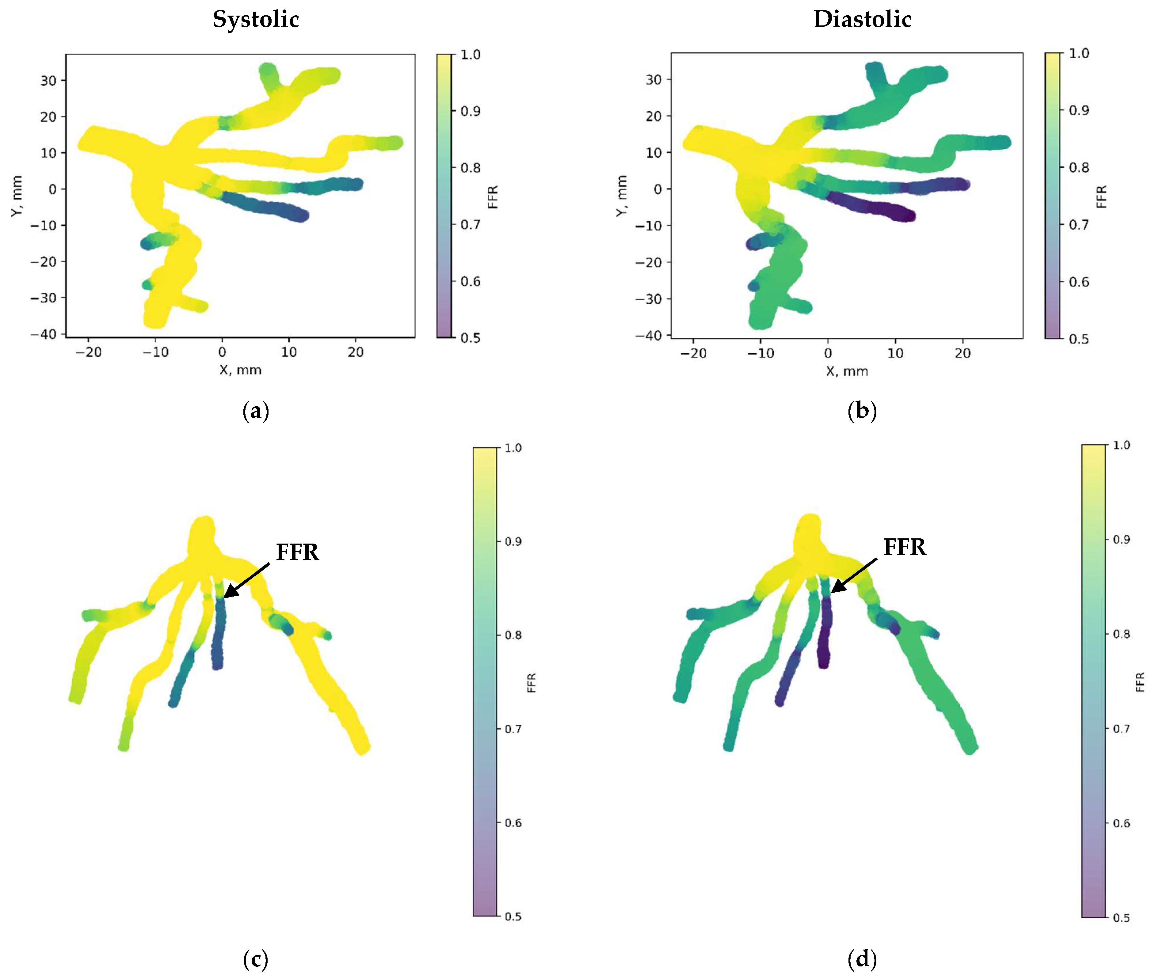
Figure 7 depicts the 3D PINN model of the CT209 coronary artery, where FFR validation is conducted at both the systolic and diastolic phases of the cardiac cycle. In Figure 7c,d, FFR values ranging between 0.9 and 0.7 are observed at the probe point, aligning with averaged invasive data for validation. This indicates an increase in the FFR to 0.9 during the systolic phase at higher pressure, followed by a decrease to 0.7 during the diastolic phase. The average FFR value of 0.77.

Figure 7.
FFR distribution in the CT209 coronary artery throughout the systolic and diastolic phases of the cardiac cycle with (a,b) 2D and (c,d) 3D views.
Figure 8 showcases the 3D PINN model of the CHN13 coronary artery, where FFR validation is performed at both the systolic and diastolic phases of the cardiac cycle. In Figure 8c,d, FFRs ranging between 0.84 and 0.6 are observed at the probe point, which is consistent with the average invasive data used for validation. This indicates an increase in the FFR to 0.84 during the systolic phase at higher pressure, followed by a decrease to 0.6 during the diastolic phase. The average FFR value of 0.67.
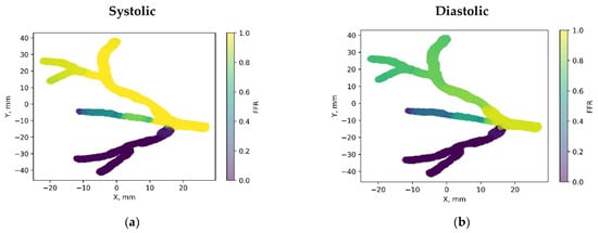
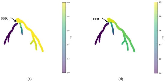
Figure 8.
FFR distribution in the CHN13 coronary artery throughout the systolic and diastolic phases of the cardiac cycle with (a,b) 2D and (c,d) 3D views.
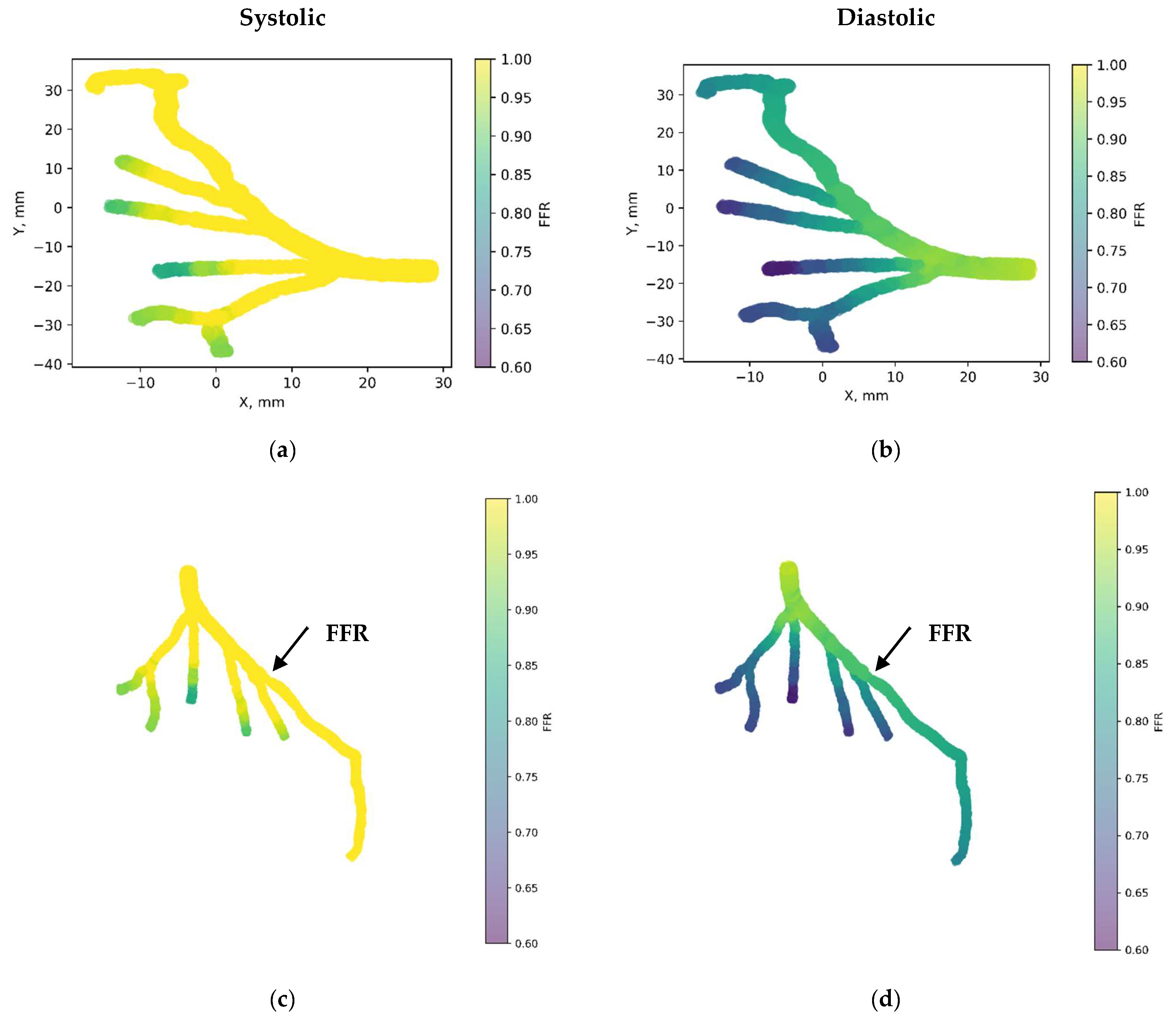
Figure 9 presents the 3D PINN model of the CHN03 coronary artery, validating the FFR at both the systolic and diastolic phases of the cardiac cycle. In Figure 9c,d, FFRs ranging between 1.1 and 0.8 are observed at the probe point, which is consistent with the average invasive data used for validation. This indicates an increase in the FFR to 1.1 during the systolic phase at higher pressure, followed by a decrease to 0.8 during the diastolic phase. The average FFR value of 0.89.
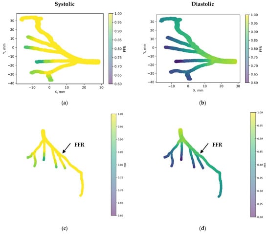
Figure 9.
FFR distribution in the CHN03 coronary artery throughout the systolic and diastolic phases of the cardiac cycle with (a,b) 2D and (c,d) 3D views.
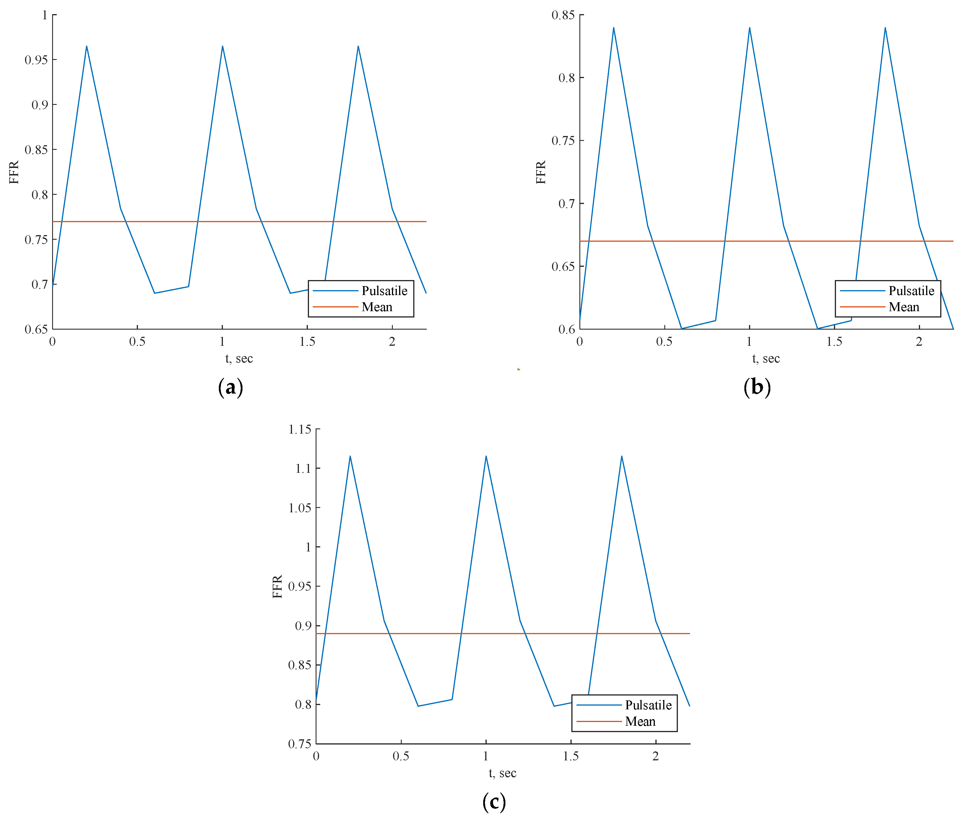
Each scenario depicted in Figure 10 exhibited a pulsatile FFR, with the resulting mean values closely compared to the invasive values, as shown in Table 4 for all three cases. The mean value error compared to invasive FFR was approximately 1.2% for CT209, 2.3% for CHN13, and 2.8% for artery CHN03. Notably, the greatest discrepancy was noted for artery CHN03 at 2.8%, consistent with errors observed in prior PBA [18], indicating its acceptability within this context. Hence, it can be inferred that the 3D Physics-Informed Neural Network (PINN) approach yielded reasonably accurate outcomes.
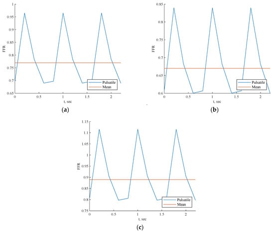
Figure 10.
FFR prediction across cardiac cycle by 3D PINN with training data for (a) CT209, (b) CHN13, and (c) CHN03.
Table 4.
The invasive FFRs values.
4.3. Three-Dimensional Artery Tree Validation without Training Data
The proposed methodology will be tested in a scenario where we consider the average inlet pressure while applying outlet boundary conditions of zero pressure. In this scenario, we examine prototypes of arterial networks depicted in Figure 2, Figure 3 and Figure 4. The key innovation lies in the fact that we do not use training data and predict the CHN03 and CT209 models based only on the training CHN13 case; therefore, by training only one model, we want to predict other models only by importing their coordinate points as an input value. The model will be trained based only on physics equations using the DeepXDE library. Additionally, a comprehensive systematic study will be conducted to assess the accuracy and robustness of the proposed method. The implementation of the proposed algorithms utilizes TensorFlow v1.10.
The 3D PINN residual history for the CHN13 artery revealed that in the current scenario, the residual values reached 10−5. This suggests that the CHN13 case exhibits satisfactory convergence, indicating accurate calculations by the code.
4.4. Fractional Flow Reserve (FFR)
Figure 11a illustrates the 3D PINN model for the CT209 coronary artery, showing FFR validation at averaged phases of the cardiac cycle. The FFR at the probe point is approximately 0.9, which does not match the average invasive value of 0.76, indicating an 18% error in the FFR.
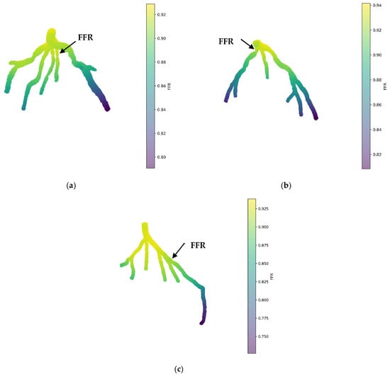
Figure 11.
FFR prediction of the mean pressure by the 3D PINN without training data for (a) CT209, (b) CHN13, and (c) CHN03.
Figure 11b displays the 3D PINN model for the CHN13 coronary artery, with FFR validation conducted at mean pressure phases of the cardiac cycle. The observed FFR value at the probe point is 0.88, which does not align with the average invasive value of 0.68, resulting in a 29% error in the FFR.
Figure 11c shows the 3D PINN model for the CHN03 coronary artery, with FFR validation performed at mean pressure phases of the cardiac cycle. The FFR value at the probe point was 0.88, closely matching the average invasive value of 0.86, indicating a 2.3% error in the FFR.
The artery used for training exhibited the largest error compared to other models that were not trained. This indicates that without training data, the PINN cannot accurately capture the unique characteristics of an artery, resulting in incorrect blood flow modeling. A PINN without training data tends to generate a pattern with higher pressure at the inlet and lower pressure at the outlets, with pressure uniformly distributed from upstream to downstream. Although the CHN03 coronary artery showed very accurate results, this is likely coincidental.
Despite these errors, there is potential for developing a universal point cloud model that can predict blood flow in various arteries without additional setup or training for each specific artery. This study aimed to demonstrate the feasibility of training a model once and using it to predict blood flow in other artery models with the same scale but different configurations, suggesting promising directions for future research.
Advances in physics-informed machine learning represent a pivotal step toward harmonizing theoretical frameworks with empirical data, a paradigm prominently exemplified in our endeavor utilizing 3D PINN for cardiovascular fluid dynamics simulations. Through the seamless fusion of physics-driven models with clinical datasets, we engineered deep neural networks capable of forecasting intricate hemodynamic parameters pivotal for CFD simulations, notably fractional flow reserve (FFR), whose noninvasive measurement poses a significant challenge. The momentum behind our adoption of 3D PINNs for CFD lies in extending the groundwork laid by [2,26], thereby enriching the approach to initializing real patient data. We acknowledge the inherent complexities in modeling intricate cardiovascular systems, particularly in capturing the nuanced dynamics of outflow boundary conditions. Our methodology capitalizes on the fundamental principles governing fluid flow in compliant arteries and supplements them with scattered CFD simulation data, thus bridging the chasm between theoretical constructs and clinical application.
Conventional 3D methodologies encounter barriers in accurately capturing the outflow boundary conditions in cardiovascular models, particularly when a cardiac network entails a variety of capillary branches interfacing with downstream microcirculation. The small diameters of these branches render experimental measurements of outflow border conditions more or less unfeasible. Consequently, conventional techniques resort to Wind–Kessel-type boundary conditions, predicated on lumped parameter models (LPMs) or lumped parameter network models (LPNMs), to approximate the intricate dynamic interplay between a network and its downstream microvasculature [27].
However, these conventional approaches accurately address the computing resistances, capacitances, and empirical correlations required for the circuit analogy theory underpinning LPMs and LPNMs. Moreover, interfacing the generated ordinary differential equations (ODEs) from these approaches with computational fluid dynamics (CFD) solvers often produces ambiguous boundary conditions, resulting in slow convergence or even numerical solution divergence.
In contrast, our approach utilizes a 3D PINN, providing a data-driven alternative to conventional methods that avoids the need for precise measurements and cumbersome parameter estimations. By integrating physics-driven models with CFD simulation data, our methodology provides a more flexible and physiologically grounded avenue for simulating blood flow in intricate cardiovascular systems.
Table 5 presents a comparison of different simulation methods in terms of their computational time and invasive FFR error percentage among all given patient arteries.
Table 5.
Comparative evaluation of computational efficiency and invasive FFR error analysis across various methods.
- CFD PBA: Utilizes computational fluid dynamics with a physiologically based algorithm. Requires significant computational resources and time, particularly for transient simulations, but achieves relatively low error rates.
- 3D PINN: Utilizes a three-dimensional physics-informed neural network. Training times are longer but still faster than CFD PBA, and prediction times are very short. Similar to 1D PINN, it depends on training data from CFD simulations and does not require outlet conditions.
In conclusion, while each method has its advantages and disadvantages, the 3D PINN method emerges as the most convenient and efficient option. It offers significantly reduced running times compared to CFD PBA, while still providing accurate results and enabling time-dependent simulations or predictions.
Despite the feasibility of previous methods like PBA, they suffered from complexity and automation issues. Our proposed method streamlined the process by requiring only mesh node coordinates and patch labelling, eliminating the need for setting up specific conditions for each artery.
In connection with conventional pure physics-based computational models, our data-driven approach circumvents the intricacies associated with mesh generation, initial and boundary condition prescriptions, and constitutive laws. By framing the problem as PDE-constrained filtering of scattered noisy data, our methodology offers flexibility and efficiency, potentially limiting the temporal transparency required to procure reliable prognoses in clinical settings. Nonetheless, challenges persist, particularly in improving the setup and training data of physics-informed neural networks and refining the accuracy and robustness of predictions.
The validation of our methodology entailed the meticulous scrutiny of a prototype arterial network and the numerical exploration of a real coronary artery tree model via CFD simulations and invasive methodologies. The integration of 3D PINN computations for outlet values in a rigid wall scenario underscored the pivotal nature of these values in resolving intricate simulations. Comparative analysis between 3D PINN and invasive methods for FFR further corroborated the consistency and accuracy of our methodology, positioning it as an invaluable tool for advancing cardiovascular simulations.
5. Conclusions
This study presents a pioneering approach to simulating fluid flow in coronary arteries using a 3D Physics-Informed Neural Network (PINN). By integrating deep learning with fundamental physics principles, the 3D PINN model accurately replicates fluid flow patterns and identifies potential areas of constriction within coronary artery networks. The model, trained using physics principles and validated against invasive mean FFR distributions, demonstrates remarkable accuracy and efficiency, outperforming the finite element method (FEM) by approximately tenfold. Further validation using Finite Element Analysis (FEA), CFD, and FSI emphasizes the versatility and importance of the 3D PINN results for various applications, suggesting a potential noninvasive and safer alternative for diagnosing coronary artery conditions, potentially superior to invasive coronary angiography (ICA).
Major Results
- Innovative 3D PINN Model:
- ◦
- Combines deep learning with fundamental physics principles.
- ◦
- Accurately replicates fluid flow patterns in coronary artery networks.
- ◦
- Identifies potential areas of constriction effectively.
- Training and Validation:
- ◦
- Trained using physics principles.
- ◦
- Validated against invasive mean FFR distributions.
- ◦
- Demonstrates exceptional accuracy and efficiency, surpassing FEM by approximately tenfold.
- Further Validation:
- ◦
- Validated using Finite Element Analysis (FEA), Computational Fluid Dynamics (CFD), and Fluid–Structure Interactions (FSI).
- ◦
- Highlights the importance of 3D PINN results for various applications.
- ◦
- Incorporates flexible nonlinear wall materials for the enhanced realism of FFRs.
- Potential for Noninvasive Diagnosis:
- ◦
- Suggests a noninvasive and safer alternative for diagnosing coronary artery conditions.
- ◦
- Potentially outperforms conventional methods like invasive coronary angiography (ICA).
- Ongoing Research:
- ◦
- Aims to refine the standalone PINN model for 3D fluid flow modeling and the diagnosis of stenosis in individual coronary arteries.
- ◦
- Introduces a novel approach for addressing experimental outflow boundary condition measurements in complex cardiac trees.
- Standalone Simulations:
- ◦
- Utilizes 3D PINN to establish standalone simulations based on physics principles and training data without requiring outlet conditions.
- ◦
- Shows promise for more effective and noninvasive stenosis diagnosis.
- Validation without Training Data:
- ◦
- Demonstrates promising results despite significant errors, indicating a physics-based approach’s potential.
- Final Outlet Conditions:
- ◦
- Determined based on tree geometry, conservation laws, numerical iterations, and patient-specific parameters.
- ◦
- Exclusively relies on 3D PINN for estimating initial conditions, setting it apart from data-driven models.
- Accuracy of 3D Artery Tree Validation with Training Data:
- ◦
- Mean value error compared to invasive FFR: 1.2% for CT209, 2.3% for CHN13, and 2.8% for CHN03.
- ◦
- Acceptable error rates, indicating reasonably accurate outcomes of the 3D PINN approach.
- Accuracy of 3D Artery Tree Validation without Training Data:
- ◦
- For CT209: 18% error in FFR.
- ◦
- For CHN13: 29% error in FFR.
- ◦
- For CHN03: 2.3% error in FFR, closely matching the average invasive value.
This approach, grounded in physiology, physics, and real-world data, shows significant promise for predicting stenosis locations and FFRs, with the potential to develop a novel numerical tool for early heart attack detection, aligning with WHO strategies for combating cardiovascular diseases globally.
Author Contributions
Conceptualization, N.A. and Y.Z.; Methodology, Y.Z.; Software, N.A. and Y.Z.; Validation, N.A.; Formal analysis, N.A.; Resources, E.Y.K.N. and Y.Z.; Data curation, N.A.; Writing—original draft, N.A.; Writing—review & editing, E.Y.K.N. and Y.Z.; Visualization, Y.Z.; Supervision, E.Y.K.N.; Project administration, Y.Z.; Funding acquisition, E.Y.K.N. All authors have read and agreed to the published version of the manuscript.
Funding
The research was supported by the Ministry of Science and Higher Education of the Republic of Kazakhstan, grant #1 number AP19678197 and grant #2 number OPCRP2022006.
Data Availability Statement
The original contributions presented in the study are included in the article, further inquiries can be directed to the corresponding author.
Acknowledgments
The authors would like to acknowledge the assistance and supply of the CT209, CHN13, and CHN03 models by Zhong Liang of the NHCS, as reported in [28]. This research was supported by two key projects: 1. CMM-SAND: Combined Multiscale/Multiphysics Experimental and Numerical Study of Sand Production Mechanisms in Oil Reservoirs (11022021CRP1506). 2. The Ministry of Science and Higher Education of the Republic of Kazakhstan under the project “Integrating Physics-Informed Neural Network, Bayesian and Convolutional Neural Networks for early breast cancer detection using thermography” (AP19678197).
Conflicts of Interest
The authors declare no conflict of interest.
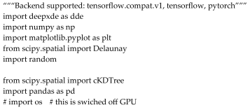
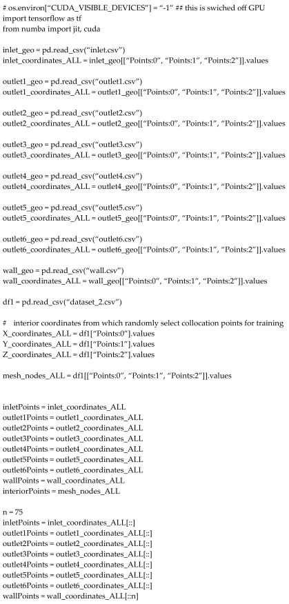
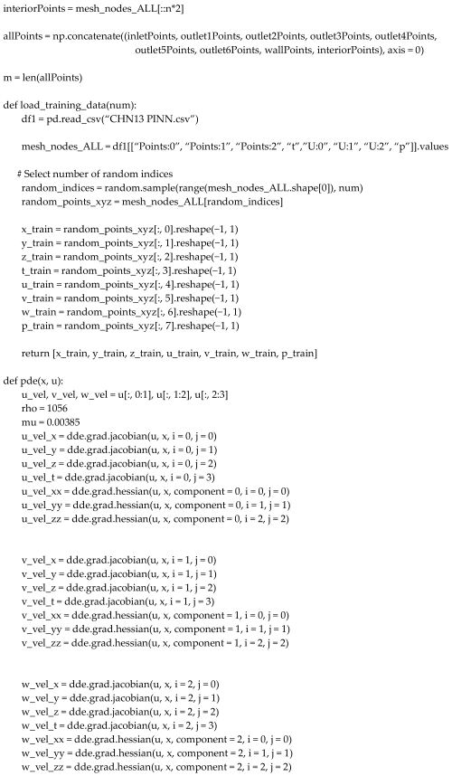
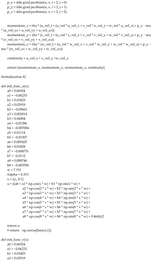
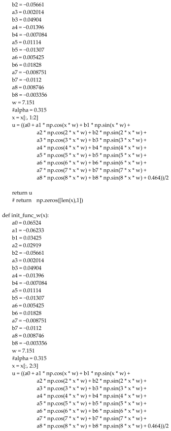
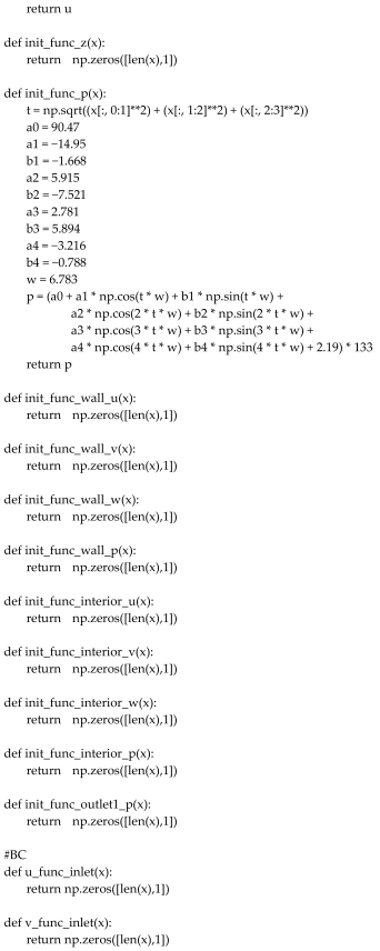
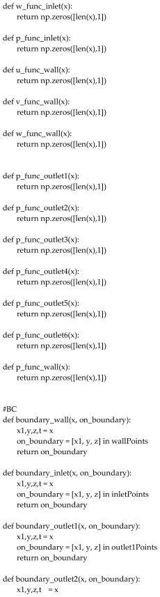
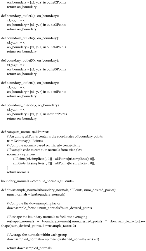
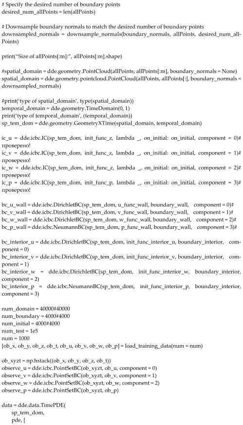
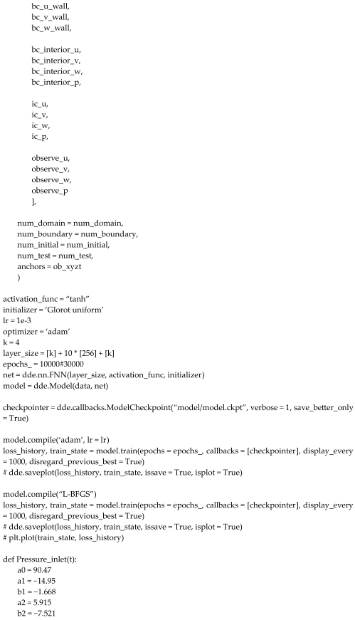
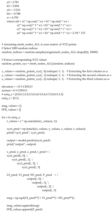
Appendix A. The 3D PINN PYTHON Code
References
- Cardiovascular Diseases (CVDs). Available online: https://www.who.int/news-room/fact-sheets/detail/cardiovascular-diseases-(cvds)?gad_source=1&gclid=CjwKCAjwoPOwBhAeEiwAJuXRhzC91fkkvSSroIMgBuzBt7BWvhkjLNgYIlo8OzlpUYmBvC5hrIDODhoC4roQAvD_BwE (accessed on 15 April 2024).
- Taebi, A. Deep learning for computational hemodynamics: A brief review of recent advances. Fluids 2022, 7, 197. [Google Scholar] [CrossRef]
- Moser, P.; Fenz, W.; Thumfart, S.; Ganitzer, I.; Giretzlehner, M. Modeling of 3D Blood Flows with Physics-Informed Neural Networks: Comparison of Network Architectures. Fluids 2023, 8, 46. [Google Scholar] [CrossRef]
- Arzani, A.; Wang, J.-X.; D’Souza, R.M. Uncovering near-wall blood flow from sparse data with physics-informed neural networks. Phys. Fluids 2021, 33, 071905. [Google Scholar] [CrossRef]
- Abdar, M.; Książek, W.; Acharya, U.R.; Tan, R.-S.; Makarenkov, V.; Pławiak, P. A new machine learning technique for an accurate diagnosis of coronary artery disease. Comput. Methods Programs Biomed. 2019, 179, 104992. [Google Scholar] [CrossRef] [PubMed]
- Chen, J.I.Z.; Hengjinda, P. Early Prediction of Coronary Artery Disease (CAD) by Machine Learning Method—A Comparative Study. March 2021, 3, 17–33. [Google Scholar]
- Li, X.; Liu, X.; Deng, X.; Fan, Y. Interplay between artificial intelligence and biomechanics modeling in the cardiovascular disease prediction. Biomedicines 2022, 10, 2157. [Google Scholar] [CrossRef] [PubMed]
- Zhang, X.; Mao, B.; Che, Y.; Kang, J.; Luo, M.; Qiao, A.; Liu, Y.; Anzai, H.; Ohta, M.; Guo, Y.; et al. Physics-informed neural networks (PINNs) for 4D hemodynamics prediction: An investigation of optimal framework based on vascular morphology. Comput. Biol. Med. 2023, 164, 107287. [Google Scholar] [CrossRef]
- Arzani, A.; Wang, J.-X.; Sacks, M.S.; Shadden, S.C. Machine Learning for Cardiovascular Biomechanics Modeling: Challenges and Beyond. Ann. Biomed. Eng. 2022, 50, 615–627. [Google Scholar] [CrossRef] [PubMed]
- Moradi, H.; Al-Hourani, A.; Concilia, G.; Khoshmanesh, F.; Nezami, F.R.; Needham, S.; Baratchi, S.; Khoshmanesh, K. Recent developments in modeling, imaging, and monitoring of cardiovascular diseases using machine learning. Biophys. Rev. 2023, 15, 19–33. [Google Scholar] [CrossRef]
- Farajtabar, M.; Larimi, M.M.; Biglarian, M.; Sabour, D.; Miansari, M. Machine Learning Identification Framework of Hemodynamics of Blood Flow in Patient-Specific Coronary Arteries with Abnormality. J. Cardiovasc. Transl. Res. 2023, 16, 722–737. [Google Scholar] [CrossRef]
- Sarabian, M.; Babaee, H.; Laksari, K. Physics-Informed Neural Networks for Brain Hemodynamic Predictions Using Medical Imaging. IEEE Trans. Med. Imaging 2022, 41, 2285–2303. [Google Scholar] [CrossRef] [PubMed]
- Isaev, A.; Dobroserdova, T.; Danilov, A.; Simakov, S. Physically Informed Deep Learning Technique for Estimating Blood Flow Parameters in Four-Vessel Junction after the Fontan Procedure. Computation 2024, 12, 41. [Google Scholar] [CrossRef]
- Lee, S.H.; Kang, S.; Hur, N.; Jeong, S.-K. A fluid-structure interaction analysis on hemodynamics in carotid artery based on patient-specific clinical data. J. Mech. Sci. Technol. 2012, 26, 3821–3831. [Google Scholar] [CrossRef]
- Nolte, D.; Bertoglio, C. Inverse problems in blood flow modeling: A review. Int. J. Numer. Method. Biomed. Eng. 2022, 38, e3613. [Google Scholar] [CrossRef] [PubMed]
- Ma, D. Quantitative Hemodynamics Using Magnetic Resonance Imaging, Computational Fluid Dynamics and Physics-Informed Neural Network; University Goettingen Repository: Goettingen, Germany, 2023. [Google Scholar]
- Du, M.; Zhang, C.; Xie, S.; Pu, F.; Zhang, D.; Li, D. Investigation on aortic hemodynamics based on physics-informed neural network. Math. Biosci. Eng. 2023, 20, 11545–11567. [Google Scholar] [CrossRef] [PubMed]
- Alzhanov, N.; Ng, E.Y.K.; Su, X.; Zhao, Y. {CFD} computation of flow fractional reserve ({FFR}) in coronary artery trees using a novel physiologically based algorithm ({PBA}) under {3D} steady and pulsatile flow conditions. Bioengineering 2023, 10, 309. [Google Scholar] [CrossRef] [PubMed]
- Raissi, M.; Karniadakis, G.E. Hidden physics models: Machine learning of nonlinear partial differential equations. J. Comput. Phys. 2018, 357, 125–141. [Google Scholar] [CrossRef]
- Raissi, M.; Perdikaris, P.; Karniadakis, G.E. Physics-informed neural networks: A deep learning framework for solving forward and inverse problems involving nonlinear partial differential equations. J. Comput. Phys. 2019, 378, 686–707. [Google Scholar] [CrossRef]
- Kingma, D.P.; Ba, J. Adam: A Method for Stochastic Optimization. arXiv 2017, arXiv:1412.6980. [Google Scholar]
- Jin, X.; Cai, S.; Li, H.; Karniadakis, G.E. NSFnets (Navier-Stokes flow nets): Physics-informed neural networks for the incompressible Navier-Stokes equations. J. Comput. Phys. 2021, 426, 109951. [Google Scholar] [CrossRef]
- Ramachandran, P.; Zoph, B.; Le, Q.V. Searching for activation functions. arXiv 2017, arXiv:1710.05941. [Google Scholar]
- Stiehm, M.; Wüstenhagen, C.; Siewert, S.; Grabow, N.; Schmitz, K.-P. Numerical simulation of pulsatile flow through a coronary nozzle model based on FDA’s benchmark geometry. Curr. Dir. Biomed. Eng. 2017, 3, 775–778. [Google Scholar] [CrossRef]
- Lu, L.; Meng, X.; Mao, Z.; Karniadakis, G.E. DeepXDE: A deep learning library for solving differential equations. SIAM Rev. 2021, 63, 208–228. [Google Scholar] [CrossRef]
- Kissas, G.; Yang, Y.; Hwuang, E.; Witschey, W.R.; Detre, J.A.; Perdikaris, P. Machine learning in cardiovascular flows modeling: Predicting arterial blood pressure from non-invasive 4D flow MRI data using physics-informed neural networks. Comput. Methods Appl. Mech. Eng. 2020, 358, 112623. [Google Scholar] [CrossRef]
- Kim, H.J.; Vignon-Clementel, I.E.; Coogan, J.S.; Figueroa, C.A.; Jansen, K.E.; Taylor, C.A. Patient-specific modeling of blood flow and pressure in human coronary arteries. Ann. Biomed. Eng. 2010, 38, 3195–3209. [Google Scholar] [CrossRef]
- Zhang, J.-M.; Zhong, L.; Luo, T.; Lomarda, A.M.; Huo, Y.; Yap, J.; Lim, S.T.; Tan, R.S.; Wong, A.S.L.; Tan, J.W.C.; et al. Simplified models of non-invasive fractional flow reserve based on {CT} images. PLoS ONE 2016, 11, e0153070. [Google Scholar] [CrossRef]


Disclaimer/Publisher’s Note: The statements, opinions and data contained in all publications are solely those of the individual author(s) and contributor(s) and not of MDPI and/or the editor(s). MDPI and/or the editor(s) disclaim responsibility for any injury to people or property resulting from any ideas, methods, instructions or products referred to in the content. |
© 2024 by the authors. Licensee MDPI, Basel, Switzerland. This article is an open access article distributed under the terms and conditions of the Creative Commons Attribution (CC BY) license (https://creativecommons.org/licenses/by/4.0/).