Dual-Parameter Prediction of Downhole Supercritical CO₂ with Associated Gas Using Levenberg–Marquardt (LM) Neural Network

Abstract

This research investigates the application of supercritical carbon dioxide (CO₂) within carbon capture, utilization, and storage (CCUS) technologies to enhance oil-well production efficiency and facilitate carbon storage, thereby promoting a low-carbon circular economy. We simulate the flow of supercritical CO₂ mixed with associated gas (flow rates 3–13 × 10⁴ Nm³/d) in a miniature venturi tube under high temperature and high-pressure conditions (30–50 MPa, 120–150 °C). Accurate fluid property calculations, essential for simulation fidelity, were performed using the R. Span and W. Wagner and GERG-2008 equations. A dual-parameter prediction model was developed based on the simulation data. However, actual measurements only provide fluid types and measurement data, such as pressure, temperature, and venturi differential pressure, to determine the liquid mass fraction (LMF) and total mass flow rate (m), presenting challenges due to complex nonlinear relationships. Traditional formula-fitting methods proved inadequate for these conditions. Consequently, we employed a Levenberg–Marquardt (LM) based neural network algorithm to address this issue. The LM optimizer excels in handling complex nonlinear problems with faster convergence, making it suitable for our small dataset. Through this approach, we formulated dual-parameter model equations to elucidate fluid flow factors, analyzing the impact of multiple parameters on the LMF and the discharge coefficient (C). The resulting model predicted dual parameters with a relative error for LMF of ±1% (Pc = 95.5%) and for m of ±1% (Pc = 95.5%), demonstrating high accuracy. This study highlights the potential of neural networks to predict the behavior of complex fluids with high supercritical CO₂ content, offering a novel solution where traditional methods fail.

1. Introduction

CCUS refers to the process where the CO₂ produced during industrial activities, such as oil and natural gas extraction, power generation, and ammonia synthesis, is captured or purified using carbon-capture technologies and then utilized in new production processes [1]. These processes include injection for enhanced oil recovery at wellheads, fire-extinguishing agents, dry-ice production, and the manufacture of various chemicals, fuels, or other valuable products [2,3,4], thereby contributing to the development of a low-carbon circular economy. Additionally, carbon sequestration ensures that CO₂ does not enter the atmosphere, with underground geological formations providing a long-term, safe storage solution [5].

For some industries, completely eliminating carbon emissions is challenging. CCUS provides a solution for these industries, aiding in achieving net-zero emission targets. While renewable energy plays a key role in reducing carbon emissions, fossil fuels will continue to be used for the foreseeable future [6]. CCUS ensures that carbon emissions from fossil fuels are minimized while transitioning to renewable energy sources. The wellhead CO₂ injection technique, with its benefits for economic efficiency, carbon reduction, and mitigating the greenhouse effect, has drawn attention from researchers and engineers. This technique not only enhances the productive life and efficiency of oil wells but also serves as a crucial method for carbon sequestration [7,8].

Supercritical CO₂ in underground flowing media is a uniform fluid with characteristics of both gas and liquid phases and is heavily influenced by operational pressure and temperature. The property data of supercritical CO₂ are vital for engineering design and process optimization. Hence, researchers continuously strive to measure and establish accurate property data to aid engineers in better designing processes involving supercritical CO₂ [9].

With a critical temperature of 30.08 °C and a critical pressure of 7.38 MPa, CO₂ easily reaches its supercritical state compared to other gases. At the critical point, CO₂ has a density of 467.6 kg/m³ and a viscosity of 3.4 × 10⁻⁵ Pa·s, resembling the density of a liquid and the viscosity of a gas. Beyond its critical point, CO₂ becomes a supercritical fluid, maintaining the properties of both the liquid and gas phases, exhibiting the viscosity of a gas and the density of a liquid.

Currently, many researchers have evaluated the computational accuracy of CO₂ property equations of state. D.P. Xi and others [10] introduced two types of property prediction models in their study: the R. Span and W. Wagner equation of state [11] and cubic equations of state. The R. Span and W. Wagner equation of state, published in 1996, is specifically designed for the accurate calculation of a wide range of CO₂ properties and phase-equilibrium parameters. This equation, based on extensive experimental data, fits the properties of pure substances and some common mixtures and extrapolates within a reasonable range. It can predict CO₂ properties, under conditions up to 800 MPa and 1100 K, such as density, viscosity, specific heat capacity, internal energy, and speed of sound.

The PR equation within the cubic equations is a commonly used property-calculation equation. This calculation method can compute the properties of mixtures by selecting appropriate mixing rules and interaction coefficients. Thus, researchers also use this classic equation for property calculations of uncommon mixtures [12,13,14]. Y.H. Yan and others [15] compared the accuracy of the BWR equation, the Exp-RK cubic equation, and the 81-type Martin–Hou equation for calculating the P-V-T properties of CO₂ under supercritical conditions. Michela Mazzoccoli and colleagues [16] compared the results of different equations, including cubic and non-analytical equations, with P-ρ-T experimental data obtained in the laboratory for CO₂ and binary mixtures of N₂, O₂, and Ar₂. Researcher Q. Wang and others [17] compared the accuracy of the Peng–Robinson (PR) equation, the standardized precipitation-kiln (SPK) equation, and the experimental precipitation-kiln (EXP-PK) equation for calculating the density, phase state, and viscosity of supercritical CO₂.

Z.R. Peng and others [18] conducted studies on supercritical CO₂ using the R. Span and W. Wagner equation of state. X. Rong and colleagues [19] compared the accuracy of the R. Span and W. Wagner equation of state with the PR equation for calculating CO₂ properties. The results calculated using the R. Span and W. Wagner method had an error of less than 3% when compared with laboratory measurements, whereas the PR equation had larger computational errors. B.J. Sun and others [20] compared the average calculation errors of density using DPR, DAK, Cranmer, PR, SPK, BWR, and R. Span and W. Wagner equations of state under supercritical drilling temperatures and pressures, where the R. Span and W. Wagner method showed the smallest error.

When calculating the physical properties of associated gas with high CO₂ content, we used the GERG-2008 equation [21]. The GERG-2008 equation is a generalized equation of state suitable for thermodynamic calculations of natural gas and natural gas mixtures, incorporating the R. Span and W. Wagner property-calculation equations. This equation has been incorporated into the international natural gas standard ISO 20765-2/3 [22]. GERG-2008 covers a pressure range of 0.03 to 99.9 MPa and can be used for property calculations of CH₄-CO₂ mixtures with molar fractions ranging from 0.06 to 0.98. The accuracy of the GERG-2008 equation has been compared with other physical property equations in the present research. M. Farzaneh-Gord et al. [23] compared the accuracy of the AGA8 equation of state with the GERG-2008 equation. The comparison results showed that the GERG-2008 equation generally had higher accuracy across all studied pressure and temperature ranges and component ranges than the AGA8 equation. D. Guerrero-Zárate et al. [24] used an iterative algorithm to compare the GERG-2008 equation with the PR, SRK, PSRK, SPHCT, and PC-SAFT equations for predicting the critical points of hydrocarbon, N₂, and CO₂ mixtures. The results indicated that the GERG-2008 equation of state could better predict critical points than some existing natural gas mixture equations of state. The research by F. Varzandeh et al. [25] showed that the GERG-2008 equation had high accuracy in calculating thermal properties, such as heat capacity and Joule–Thomson coefficients, for pure components and multicomponent mixtures over a wide range of pressures and temperatures.

From an engineering perspective, the study of supercritical CO₂ fluid is of significant importance because of its excellent solvency. The applications of its solubility properties have been explored, such as in the production of biofuels, chemicals, and pharmaceuticals [26,27,28]. Additionally, supercritical CO₂ is frequently utilized in catalyst preparation and reaction engineering, with ongoing studies into the kinetics and mechanisms of catalytic reactions under these conditions to enhance the efficiency and selectivity of the reactions [29,30,31]. Moreover, investigations have been conducted on the heat-transfer characteristics of supercritical CO₂ to optimize energy-conversion and storage processes. For instance, the development of supercritical CO₂ Brayton cycle power-generation technology as an efficient energy-conversion system has been a focal point of research [19]. J.L. Yang [32] analyzed the heat-transfer principles, characteristics, and mechanisms of supercritical CO₂ fluids. M. van der Kraan and others [33] performed computational fluid-dynamics simulations of heated supercritical CO₂ flowing upward or downward in vertical tubes, studying the effects of temperature-induced physical property changes and buoyancy on heat transfer. V.A. Kurganov and colleagues [34] conducted experimental studies on the turbulent heat transfer in tubes heated with supercritical CO₂ fluid.

Supercritical CO₂ also holds considerable potential in environmental protection projects, aiding in mitigating environmental issues. For example, CCUS can reduce greenhouse-gas emissions and treat wastewaters, such as supercritical water. Researchers like B.J. Sun [20] studied the property changes of supercritical CO₂ injected into wellbores. R.N. Wu and others [35] explored the use of supercritical CO₂’s solubility in heavy oil to reduce crude oil’s viscosity and improve its properties. Jhoan M.C. Cubas and others [36] investigated the injection of supercritical CO₂ into reservoirs using centrifugal pumps. W. Harbert and others [37] conducted detailed 4D seismic imaging of the injection points at the wellhead to aid in the development of CO₂ sequestration techniques and methods for different regions and geological structures. S. Bouzgarrou and others [38] used numerical methods to study the storage capacity of deep saline aquifers under supercritical conditions. A. Belhocine and others [39] numerically predicted free convection and mixed convection heat transfer from a non-isothermal vertical flat plate to supercritical water. S. Xin and others [40] simulated the transient behavior of printed circuit heat exchangers (PCHEs) in the Brayton cycle. J. Tan and others [41] reviewed experimental studies on supercritical CO₂ for viscosity reduction in heavy oils, summarizing the mechanisms and main factors influencing viscosity reduction by supercritical CO₂.

Despite numerous research on the flow mechanisms of supercritical CO₂ having been published, the challenge of measuring flow parameters of downhole supercritical CO₂ has not been fully addressed. This study, through comparative research, identified REFPROP [42] as the property-calculation method and determined the structural parameters of Venturis based on simulation results from the LedaFlow [43] transient multiphase flow simulator. Conducting simulation experiments on supercritical CO₂-associated gas downhole, the study analyzed the relationship between liquid mass fraction, discharge coefficient, and ratios of front differential pressure to upstream pressure, front differential pressure to total pressure loss, flow rate, temperature, and pressure.

In recent years, the rise of artificial neural network algorithms has challenged traditional modeling methods based on theoretical equations. When the coupling degree between parameters is high or the relationship between variables is nonlinear, it is often difficult to get the ideal effect from the modeling method based on a theoretical equation. However, the artificial neural network algorithm overcomes this drawback, and it is composed of adaptive neurons connected as neural networks to achieve the purpose of experiential learning [44,45]. ANNs can process a variety of large-scale data, exhibiting strong capabilities in self-learning, self-organization, self-adaptation, and nonlinear mapping. Therefore, an LM neural network method was employed to construct a dual-parameter model for liquid content and total flow rate.

Section 2 of this paper describes the calculation method for the simulated property parameters. Section 3 details the structure of the sensor and performs simulation calculations by LedaFlow, analyzes data, and identifies the most critical modeling parameters. Section 4 establishes a dual-parameter model for flow rate and water content using the LM neural network and analyzes the results.

2. CO₂ Property Calculation

In the downhole flowing media, supercritical CO₂ is a uniform fluid that exhibits characteristics of both the gas and liquid phases, with its density significantly influenced by the operational pressure and temperature. To ensure that simulations can accurately predict the fluid’s flow characteristics, it is essential to analyze the property parameters of CO₂.

2.1. Comparison of CO₂ Property-Calculation Methods

Over the past few decades, extensive research on CO₂ property-calculation equations has been conducted. The R. Span and W. Wagner equation of state is specifically designed for the accurate calculation of a wide range of CO₂ properties and phase-equilibrium parameters. Due to its small calculation error and wide applicability, meeting the practical engineering calculation needs, the R. Span and W. Wagner equation of state has also been widely used in the engineering field.

Some commonly used physical properties calculation equations have been integrated into several commercial software packages, such as REFPROP, PVTsim Version 20.0 [46], and Multiflash Version 6.2 [47]. REFPROP Version 9.1 is an internationally recognized authoritative software for the calculation of fluid properties developed by the National Institute of Standards and Technology (NIST) in the USA. It includes the latest standards for calculating the properties of natural gases and other substances and integrates the R. Span and W. Wagner property-calculation model. PVTsim, developed by the Danish conglomerate Calsep, is a PVT simulation software that includes some common property-calculation equations, such as PR, SRK, and PR78 equations. Multiflash, developed by KBC Advanced Technologies in the UK, is a multifunctional PVT simulation and analysis software, containing cubic equations, high-precision cubic equations, and some international standard property models.

Table 1. Results and relative errors of CO₂ property-calculation methods at 30 MPa, with density in units of kg/m³ and viscosity in Pa·s.

	T °C	116.85	126.85	136.85	146.85
Calculation Methods
R. and W.	ρ	596.59	561.50	529.46	500.50
	Viscosity	4.79 × 10−5	4.51 × 10−5	4.27 × 10−5	4.08 × 10−5
PVTsim	ρ	578.75	544.57	513.91	486.50
	RE	−2.99%	−3.02%	−2.94%	−2.80%
	Viscosity	5.61 × 10−5	5.25 × 10−5	4.95 × 10−5	4.70 × 10−5
	RE	17.12%	16.41%	15.93%	15.20%
Multiflash	ρ	571.28	537.99	508.08	481.29
	RE	−4.24%	−4.19%	−4.04%	−3.84%
	Viscosity	4.85 × 10−5	4.56 × 10−5	4.33 × 10−5	4.14 × 10−5
	RE	1.25%	1.11%	1.31%	1.37%

presents the calculation results and relative errors of various property-calculation methods, referencing the CO₂ density and viscosity data from the appendices of the R. Span and W. Wagner paper, for pressures of 30 MPa and temperatures ranging from 116.85 to 146.85 °C. In the table, R. and W. refers to the R. Span and W. Wagner equation of state, with density in units of kg/m³ and viscosity in Pa·s.

The data from Table 1 indicates that, within the range of 30 MPa and temperatures from 116.85 to 146.85 °C, the CO₂ density values listed in the appendices of the R. Span and W. Wagner paper range between 500.50 and 596.59 kg/m³, and the viscosity values are between 4.08 × 10⁻⁵ and 4.79 × 10⁻⁵ Pa·s. At these conditions, CO₂ is in a supercritical state. The relative error range for the density calculations by PVTsim is between −3.02% and −2.80%, and for viscosity calculations, it is between 15.20% and 17.12%. The relative error range for the density calculations by Multiflash is between −4.24% and −3.84%, and for the viscosity calculations, it is between 1.11% and 1.37%. The error-analysis results suggest that common commercial property-calculation methods exhibit significant errors in calculating CO₂ property parameters. The results in Table 1 demonstrate that the REFPROP software can provide accurate CO₂ property-calculation results.

Given the high methane content in the downhole gas injection working fluid, it becomes necessary to calculate the properties of the mixed fluid. The GERG-2008 equation [21] was widely used for the mixture properties calculations in the situation, which is also integrated into the REFPROP software.

Table 2. Results and relative errors of CO₂-CH₄ mixture property-calculation methods at 30 MPa, with density in units of kg/m³ and viscosity in Pa·s.

	T °C	116.85	126.85	136.85	146.85
Calculation Methods
REFPROP	ρ	311.3	298.42	286.66	275.91
	Viscosity	3.06 × 10−5	3.01 × 10−5	2.97 × 10−5	2.94 × 10−5
PVTsim	ρ	313.08	300.21	288.46	277.71
	RE	0.57%	0.60%	0.63%	0.65%
	Viscosity	3.29 × 10−5	3.23 × 10−5	3.17*10−5	3.13 × 10−5
	RE	7.71%	7.16%	6.67%	6.24%
Multiflash	ρ	303.80	291.37	280.03	269.66
	RE	−2.41%	−2.36%	−2.31%	−2.26%
	Viscosity	3.10 × 10−5	3.04 × 10−5	3.00 × 10−5	2.96 × 10−5
	RE	1.21%	0.96%	0.81%	0.75%

presents the calculation results and relative errors of various property-calculation methods, referencing the density and viscosity data of the CO₂-CH₄ mixture (molar fractions = 50:49.85) calculated using the REFPROP software.

The data from Table 2 show that, within a pressure of 30 MPa and temperatures ranging from 116.85 to 146.85 °C, the density of the CO₂-CH₄ mixture falls between 275.91 and 311.3 kg/m³, while the viscosity ranges from 2.94 × 10⁻⁵ to 3.06 × 10⁻⁵ Pa·s. Compared to the physical properties data of CO₂ in Table 1, the CO₂-CH₄ mixture exhibits lower density and viscosity under the same conditions.

Under these conditions, the CO₂-CH₄ mixture is in a supercritical state. The relative error for density calculations by PVTsim ranges from 0.57% to 0.65%, and for viscosity calculations, it ranges from 6.24% to 7.71%. The relative error for density calculations by Multiflash is between −2.41% and −2.26%, and for viscosity calculations, it is between 0.75% and 1.21%. The results in Table 1 and Table 2 demonstrate that REFPROP software, which incorporates the GERG-2008 equation, can provide accurate property calculations for CO₂ and CO₂-CH₄ mixtures. In the subsequent simulation experiments and actual flow experiments, the CO₂ and associated gas density calculations will utilize the REFPROP software.

2.2. Downhole Working Fluid Property-Calculation Results

In the downhole conditions ranging from 30 to 50 MPa and 120 to 150 °C,

Table 3. Density and viscosity table for supercritical CO_2, with density in units of kg/m³ and viscosity in Pa·s.

	T °C	120	130	140	150
P MPa
30	ρ	585.22	551.07	520.01	491.99
	Viscosity	4.69 × 10−5	4.43 × 10−5	4.21 × 10−5	4.03 × 10−5
40	ρ	692.87	662.75	634.12	607.11
	Viscosity	5.84 × 10−5	5.54 × 10−5	5.27 × 10−5	5.03 × 10−5
50	ρ	763.68	737.19	711.57	686.94
	Viscosity	6.80 × 10−5	6.46 × 10−5	6.16 × 10−5	5.90 × 10−5

presents the results of the supercritical CO₂ density and viscosity calculated using the REFPROP software.

From Table 3, it is observed that, under the specified conditions, supercritical CO₂ exhibits the density of a liquid and the viscosity of a gas, with density values ranging from 491.99 to 763.68 kg/m³ and viscosity values from 4.03 × 10⁻⁵ to 6.80 × 10⁻⁵ Pa·s. When the temperature is held constant, an increase in pressure leads to a simultaneous increase in both the density and viscosity of CO₂. Conversely, when the pressure is held constant, an increase in temperature results in a decrease in both the density and viscosity of CO₂.

Under downhole conditions ranging from 30 to 50 MPa and 120 to 150 °C, the molar ratio of the CO₂-CH₄ mixture is 50:49.85.

Table 4. Mixed density and viscosity table for CO₂ and CH₄, with density in units of kg/m³ and viscosity in Pa·s.

	T °C	120	130	140	150
P MPa
30	ρ	307.11	294.6	283.17	272.71
	Viscosity	3.04 × 10−5	3.00 × 10−5	2.96 × 10−5	2.93 × 10−5
40	ρ	379.28	365.93	353.44	341.77
	Viscosity	3.61 × 10−5	3.54 × 10−5	3.47 × 10−5	3.42 × 10−5
50	ρ	433.11	420.05	407.64	395.86
	Viscosity	4.07 × 10−5	3.97 × 10−5	3.89 × 10−5	3.82 × 10−5

presents the mixed density and viscosity results calculated using the REFPROP software.

According to Table 4, under the specified conditions, the density of the CO₂-CH₄ mixture ranges between 272.71 and 433.11 kg/m³, and the viscosity ranges between 2.93 × 10⁻⁵ and 4.07 × 10⁻⁵ Pa·s. With the temperature held constant, an increase in pressure leads to an increase in both the density and viscosity of the CO₂-CH₄ mixture. Conversely, with the pressure held constant, an increase in temperature results in a decrease in both the density and viscosity of the mixture. Compared to the properties of supercritical CO₂ under the same conditions, the CO₂-CH₄ mixture exhibits lower density and lower viscosity.

3. Simulation of Supercritical CO₂ with Associated Gas

In the typical conditions of downhole gas injection, the pressure range is 30 to 50 MPa, the temperature range is 120 to 150 °C, and the flow rate range is 3 to 13 × 10⁴ Nm³/d. The flowing medium consists of mixtures of supercritical CO₂ and CH₄ in varying proportions. This section designs homogeneous flow simulation experiments within these operational ranges, with the liquid mass fraction (LMF) representing the mass fraction of CO₂ between 23.40% and 96.12%. The study analyzes how the LMF and discharge coefficient C vary with changes in flow rate, pressure, temperature, and other flow parameters.

3.1. The Structure of Miniature Venturi Tube

In our prior investigation [42], we considered both simulation results and determined the optimal configuration for a miniature Venturi sensor. This design features an inlet diameter (D) of 15 mm, a throttling ratio value (β) of 0.4, and a throat diameter (d) of 6 mm. Adhering to the specifications outlined in the ISO 5167-4 [48] international standard, key design parameters encompass a contraction angle of 21°, an expansion angle of 7°, a straight tube section before the throat of 10 D, a throat length of 1 d, a straight tube section after the throat of 6 D, and a wall roughness of 0.006 mm.

Illustrated in Figure 1 are three pressure-tapping points, labeled P₁, P₂, and P₃, strategically positioned to enhance pressure measurement accuracy. The differential pressures across the front and rear sections of the Venturi are represented by Δp₁ and Δp₂, respectively, while the overall pressure loss is denoted as Δp_loss. The subsequent simulation work is based on the structure of this miniature Venturi sensor.

3.2. Simulation Conditions

Table 5. Homogeneous flow simulation conditions for supercritical CO₂ downhole-associated gas.

P MPa	T °C	F × 104 Nm3/d	U m/s	CO2 mol%	LMF %	LVF %	Re × 106	${\rho }_{\mathit{l}}/{\rho }_{\mathit{g}}$
30	120	2.5~13.0	5.5~38.8	10, 20, 30, 40, 50, 60, 70, 80, 90	23.4, 40.7, 54.1, 64.7, 73.3, 80.5, 86.5, 91.7, 96.1	7.0~85.9	0.8~5.4	4.1
	130	2.5~13.0	5.8~40.1	10, 20, 30, 40, 50, 60, 70, 80, 90	23.4, 40.7, 54.1, 64.7, 73.3, 80.5, 86.5, 91.7, 96.1	7.2~86.3	0.9~5.6	4.0
	140	2.5~13.0	6.1~41.4	10, 20, 30, 40, 50, 60, 70, 80, 90	23.4, 40.7, 54.1, 64.7, 73.3, 80.5, 86.5, 91.7, 96.1	7.4~86.6	0.9~5.8	3.8
	150	2.5~13.0	6.5~42.7	10, 20, 30, 40, 50, 60, 70, 80, 90	23.4, 40.7, 54.1, 64.7, 73.3, 80.5, 86.5, 91.7, 96.1	7.5~86.9	0.9~5.9	3.7
40	120	2.5~13.0	4.6~31.2	10, 20, 30, 40, 50, 60, 70, 80, 90	23.4, 40.7, 54.1, 64.7, 73.3, 80.5, 86.5, 91.7, 96.1	7.3~86.5	0.7~4.2	3.86
	130	2.5~13.0	4.8~32.2	10, 20, 30, 40, 50, 60, 70, 80, 90	23.4, 40.7, 54.1, 64.7, 73.3, 80.5, 86.5, 91.7, 96.1	7.4~86.7	0.7~4.4	3.81
	140	2.5~13.0	5.0~33.1	10, 20, 30, 40, 50, 60, 70, 80, 90	23.4, 40.7, 54.1, 64.7, 73.3, 80.5, 86.5, 91.7, 96.1	7.5~86.9	0.8~4.6	3.75
	150	2.5~13.0	5.2~34.1	10, 20, 30, 40, 50, 60, 70, 80, 90	23.4, 40.7, 54.1, 64.7, 73.3, 80.5, 86.5, 91.7, 96.1	7.7~87.0	0.9~4.9	3.69
50	120	2.5~13.0	4.1~27.0	10, 20, 30, 40, 50, 60, 70, 80, 90	23.4, 40.7, 54.1, 64.7, 73.3, 80.5, 86.5, 91.7, 96.1	7.7~87.0	0.7~3.9	3.69
	130	2.5~13.0	4.3~27.8	10, 20, 30, 40, 50, 60, 70, 80, 90	23.4, 40.7, 54.1, 64.7, 73.3, 80.5, 86.5, 91.7, 96.1	7.7~87.1	0.7~4.0	3.65
	140	2.5~13.0	4.4~28.5	10, 20, 30, 40, 50, 60, 70, 80, 90	23.4, 40.7, 54.1, 64.7, 73.3, 80.5, 86.5, 91.7, 96.1	7.8~87.3	0.7~4.2	3.62
	150	2.5~13.0	4.6~29.2	10, 20, 30, 40, 50, 60, 70, 80, 90	23.4, 40.7, 54.1, 64.7, 73.3, 80.5, 86.5, 91.7, 96.1	7.9~87.4	0.7~4.3	3.58

presents the simulation conditions for the homogeneous flow of supercritical CO₂ downhole-associated gas. There is a total of 540 simulation points, with the flowing medium being associated gas, which is a mixture of supercritical CO₂ and CH₄ in varying proportions.

The pressure P and temperature T ranges are the same as those discussed in Section 3.2, with the flow rate F ranging from 2.5 to 13 × 10⁴ Nm³/d. The liquid mass fraction LMF (i.e., the mass fraction of CO₂) ranges from 23.40% to 96.12%, which translates to a Volume Liquid Fraction LVF range of 7.0% to 87.4%, indicating a wide range of liquid content. In these simulation conditions, the density range for supercritical CO₂ is 492.0 to 763.7 kg/m³, the density range for methane CH₄ is 131.3 to 207.1 kg/m³, and the mixed density range for the associated gas is 156.4 to 685.4 kg/m³, with a liquid-to-gas density ratio range of 3.58 to 4.1.

3.3. Analysis of Influencing Factors for LMF and C

To establish models for the discharge coefficient (C) and the liquid mass fraction (LMF), this section analyzes the relationship between important operational parameters, such as density, flow rate, pressure, and temperature, with C and LMF based on simulation results. This analysis identifies the parameters required for modeling, laying the foundation for the subsequent neural network modeling.

3.3.1. Relationship between LMF and Various Flow Parameters

• The influence of LMF on Δp/p under constant pressure;

Figure 1 illustrates the relationship between the liquid mass fraction (LMF) and the ratio of front differential pressure to upstream pressure(Δp/p), categorized by pressure. The horizontal axis represents LMF, ranging from 20% to 100%, and the vertical axis represents the ratio of front differential pressure to upstream pressure(Δp/p), with a range from 0 to 0.6. These pictures display data for a pressure range of 30 to 50 MPa, a temperature range of 120 to 150 °C, and a flow rate range of 2.5 to 13 × 10⁴ Nm³/d.

From Figure 2, examining the curves at any given pressure, such as in Figure 2a, it is generally observed that, at 30 MPa, the LMF exhibits a monotonically increasing relationship with Δp/p. When the temperature is constant, an increase in the flow rate, i.e., faster flow velocity, results in a higher front differential pressure, and the curve of the relationship between LMF and Δp/p shifts upwards. Conversely, with a constant flow rate, an increase in temperature reduces the fluid density, and the curve shifts upwards. The trends in Figure 2b,c are consistent with Figure 2a.

• The influence of LMF on Δp/Δp_loss under constant pressure;

Figure 3 presents the relationship between liquid mass fraction (LMF) and the ratio of front differential pressure to total pressure loss (Δp/Δp_loss) categorized by pressure. The horizontal axis represents LMF, ranging from 20% to 100%, and the vertical axis represents Δp/Δp_loss, ranging from 1.90 to 3.66.

Observing the curves under any given pressure in Figure 3, such as in Figure 3a, it is generally seen that, at 30 MPa, the LMF exhibits a monotonically changing relationship with Δp/Δp_loss. When the temperature is constant, the curve of the relationship between LMF and Δp/Δp_loss shifts downwards with an increase in the flow rate. Conversely, with a constant flow rate, the curve shifts upwards as the temperature increases. The trends in Figure 3b,c are consistent with Figure 3a.

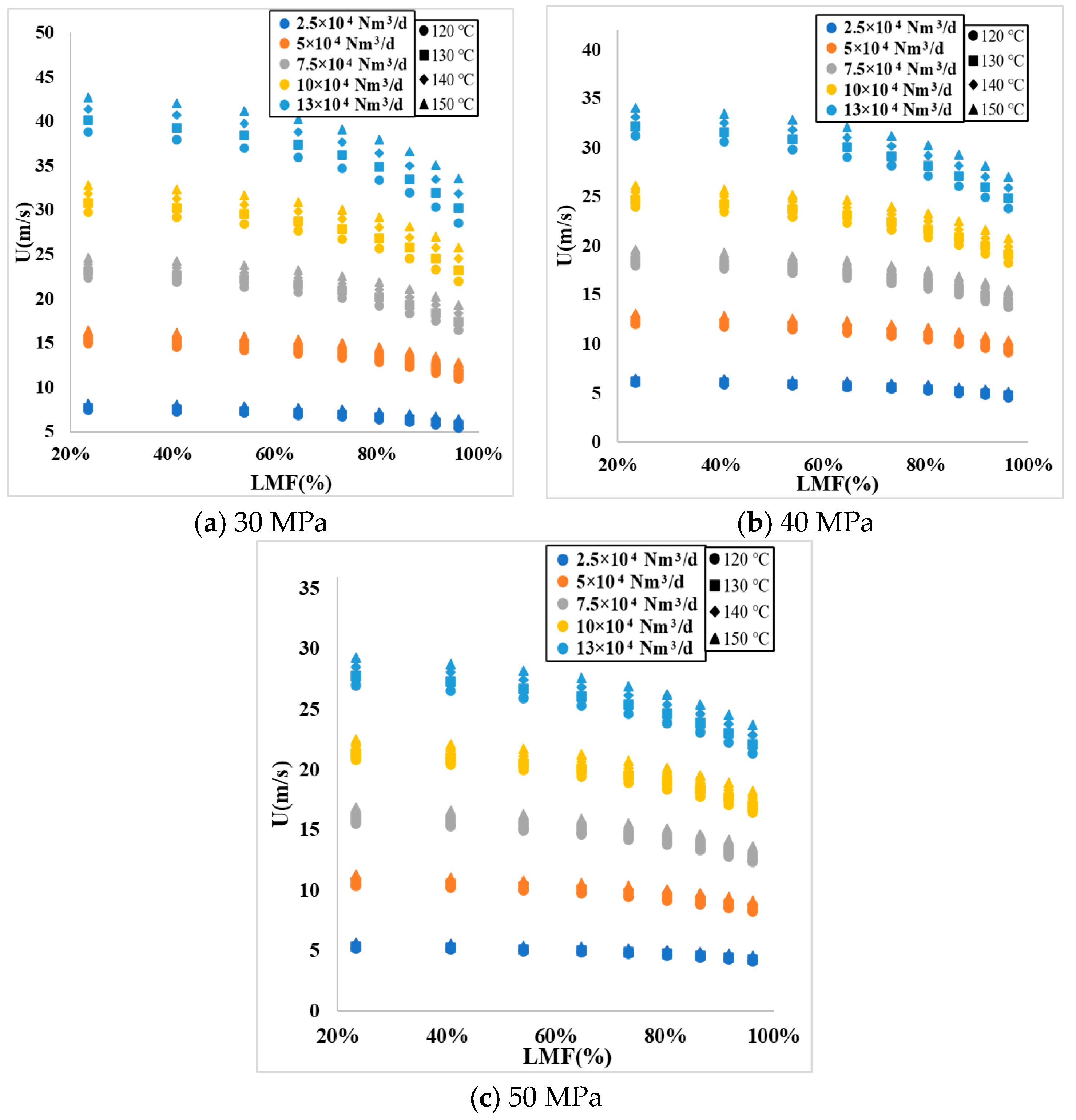
• The influence of LMF on U under constant pressure;

Figure 4 categorizes the relationship between the liquid mass fraction (LMF) and flow velocity U by pressure. The horizontal axis is the LMF, ranging from 20% to 100%, and the vertical axis is the flow velocity U, ranging from 0 to 45 m/s.

From Figure 4, observing the curves at any given pressure, like in Figure 4a, it is noted that, at 30 MPa, there is a generally monotonically decreasing relationship between LMF and the flow velocity U. With constant temperature, the curve of the relationship between LMF and U shifts downwards as the flow rate increases. With a constant flow rate, the curve shifts upwards as the temperature increases. The patterns in Figure 4b,c are consistent with Figure 4a.

The above analysis indicates that the factors Δp/p, Δp/Δp_loss, U, P, and T have a systematic impact on LMF, and P and T, along with the components, determine the liquid–gas density ratio ρ_l/ρ_g. Therefore, the function predicting LMF can be represented by Equation (1).

$$LMF=f_1({\displaystyle \frac{\Delta p}{p}},{\displaystyle \frac{\Delta p}{\Delta p_{loss}}},U,{\displaystyle \frac{{\rho }_l}{{\rho }_g}})$$

(1)

3.3.2. Relationship between Discharge Coefficient C and Various Flow Parameters

Figure 5 illustrates the influence of the Reynolds number (Re) on the discharge coefficient (C) across all simulated conditions. The horizontal axis represents Re, ranging from 0 to 7 × 10⁶, while the vertical axis is for C, ranging from 0.7 to 0.9.

The legend in the lower left corner of Figure 5 indicates that the size of the scatter points represents the magnitude of pressure (30 MPa, 40 MPa, and 50 MPa with decreasing scatter size, respectively). Different colors represent different temperatures (yellow for 120 °C, gray for 130 °C, orange for 140 °C, blue for 150 °C), and different symbols represent the flow rates (horizontal line for 2.5 × 10⁴ Nm³/d, diamond for 5.0 × 10⁴ Nm³/d, triangle for 7.5 × 10⁴ Nm³/d, circle for 10.0 × 10⁴ Nm³/d, square for 13.0 × 10⁴ Nm³/d).

First, the influence of LMF variation on C is observed (top-right subplot). Under unchanged conditions, such as 30 MPa, 120 °C, 13.0 × 10⁴ Nm³/d, Re and C exhibit a generally monotonically increasing relationship, as indicated by the red circle in the lower right corner of the figure. The top-right corner plots the relationship between LMF and C under these conditions, showing that C monotonically increases with an increasing LMF.

Second, the effect of pressure changes on C is observed (lower-left subplot). With other conditions constant, as the pressure increases, the relationship curve of Re and C contracts towards the upper left. The lower left shows an enlarged view of some curves, illustrating that the curves contract upwards as the pressure increases.

Third, the impact of temperature changes on C is examined. With other conditions constant, as the temperature increases, the relationship curve of Re and C expands downwards.

Lastly, the influence of flow rate changes on C is reviewed. With other conditions constant, as the flow rate increases, the relationship curve of Re and C expands downwards.

A comprehensive observation of Figure 5 reveals clear patterns in the relationships between LMF, pressure, temperature, flow rate, and C. Subsequently, the relationships between velocity, LMF, and C are separately analyzed to further explore these patterns.

• The influence of flow velocity U on the discharge coefficient C;

Figure 6 shows the impact of flow velocity on C across all simulated conditions. The horizontal axis is the flow velocity, ranging from 0 to 45 m/s, and the vertical axis is C, ranging from 0.67 to 0.89.

In Figure 6, different colors and shapes indicate different pressures, with blue circles for 30 MPa, orange squares for 40 MPa, and gray circles for 50 MPa.

With constant pressure, the relationship between flow velocity and C shows a monotonically decreasing trend. As the pressure varies, the range of operational flow velocities widens with decreasing pressure; at 30 MPa, the curve-relating flow velocity to C shifts downward, with its higher flow velocity portion overlapping with the curves at 40–50 MPa.

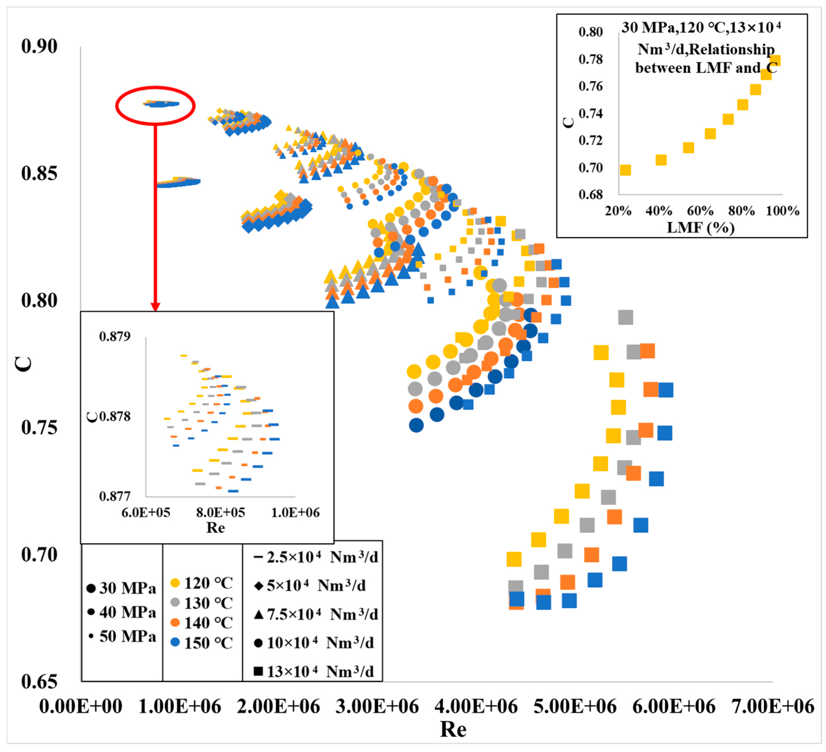
• The influence of LMF on the discharge coefficient C under constant pressure.

Figure 7 illustrates the impact of LMF on C across all simulated conditions. The horizontal axis represents LMF, ranging from 20 to 100%, and the vertical axis is C, ranging from 0.67 to 0.88.

From Figure 7, examining the curves at any given pressure, like in Figure 7a, it is observed that LMF and C generally have a monotonically increasing relationship. With constant temperature, the relationship curve between LMF and C shifts downwards as the flow rate increases. With constant flow rate, the relationship curve between LMF and C also shifts downwards as the temperature increases, with a zoomed-in view of some curves at the bottom. The patterns in Figure 7b,c are consistent with Figure 7a.

The analysis indicates that LMF, flow velocity (U), pressure (P), and temperature (T) have systematic influences on C, P, and T, along with the components and determine the liquid–gas density ratio. Hence, a function predicting LMF can be represented by Equation (2).

$$C=f_2(LMF,U,{\displaystyle \frac{{\rho }_l}{{\rho }_g}})$$

(2)

4. Dual-Parameter Prediction Method of Supercritical CO₂ Associated Gas

The previous sections analyzed the changing characteristics of the liquid mass fraction (LMF) and the discharge coefficient (C) with various flow parameters. This section aims to construct a homogeneous flow liquid mass fraction (LMF) measurement model and a dual-parameter model for the total mass flow rate (m) based on the Levenberg–Marquardt (LM) artificial neural network (ANN) method and to evaluate the predictive accuracy of the model.

4.1. LM Neural Network Method and Dual-Parameter Influence Factor Equations

Artificial neural networks (ANNs), a subset of machine learning and the core of deep learning algorithms, consist of adaptable neurons. They mimic the method of signal transmission between biological neurons, connecting in a network to achieve experiential learning. A typical neural network architecture includes input, hidden, and output layers, with neurons in the hidden and output layers possessing activation functions. There are no intra-layer or cross-layer connections between neurons, and such a network structure is often referred to as a “multilayer feedforward neural network”. In this study, model fitting is implemented based on Matlab’s (2019b) Neural Network Fitting toolbox, which utilizes the Levenberg–Marquardt algorithm (LM) [49].

The variations in LMF and C, as analyzed previously, show complex patterns influenced by multiple parameters. In practical measurement scenarios, the flow velocity (U) is an unknown quantity in the function composing the homogeneous flow LMF and C, hence necessitating the use of other measurement parameters for assistance. This subsection establishes a dual-parameter model for the homogeneous flow LMF and the total mass flow rate (m) using the LM neural network method, with the dual-parameter influence factor equations presented as Equation (3).

$$\left\{\begin{array}{l}LMF=f_1({\displaystyle \frac{\Delta p}{p}},{\displaystyle \frac{\Delta p}{\Delta p_{loss}}},U,{\displaystyle \frac{{\rho }_l}{{\rho }_g}})\\ C=f_2(LMF,U,{\displaystyle \frac{{\rho }_l}{{\rho }_g}})\\ {\rho }_{mix}=f_3({\rho }_g,{\rho }_l,LMF)\\ m={\displaystyle \frac{C{\beta }^2}{\sqrt{1-{\beta }^4}}}\epsilon {\displaystyle \frac{\pi D^2}{4}}\sqrt{2{\rho }_{mix}\Delta p}\\ U={\displaystyle \frac{m}{A{\rho }_{mix}}}\end{array}\right\}$$

(3)

In this equation, flow velocity (U) is combined with the total mass flow rate (m) and the mixture density ρ_l/ρ_g to be determined. Therefore, parameters such as Δp, Δp/p, Δp/Δp_loss, ρ_g, ρ_l, and ρ_l/ρ_g are used as input values for the neural network, with LMF and m as the output values.

The data are divided into training, validation, and test sets, retaining the default settings. The training set is used to compute the gradient and update connection weights and biases; the validation set is used to verify the network’s generalization and to stop training before overfitting; the test set is used for the independent testing of network generalization.

All 540 simulated data points are used, with the operational pressure P ranging from 30 to 50 MPa, temperature T from 120 to 150 °C, flow rate F from 2.5 to 13 × 10⁴ Nm³/d, and LMF ranging from 23.40 to 96.12%. The training dataset includes 432 data points, the validation dataset includes 54 data points, and the test dataset includes 54 data points. The network employs three hidden layers, with the Sigmoid activation function, and a linear transfer function for the output layer. The LM algorithm optimizes training, stopping the training if the validation error increases consistently over six iterations, with a maximum of 1000 iterations; 20, 15, and 10 are determined as the neuron numbers of the three hidden layers, respectively.

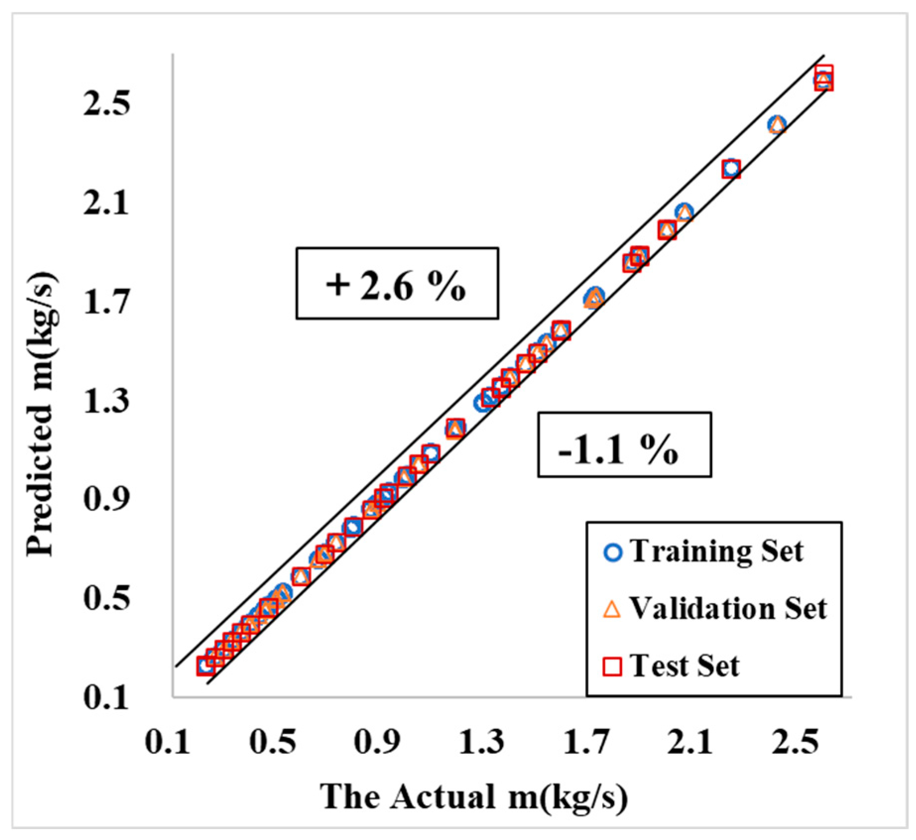
4.2. Prediction Results and Error Analysis

To quantitatively evaluate the predictive performance of the model, and take the prediction performance of LMF as an example, the definition of relative error (Rel) is introduced as follows.

$$RE={\displaystyle \frac{LM{F}_e-LM{F}_p}{LM{F}_e}}$$

(4)

In Equation (4), LMF_e represents the true LMF value inputted into the simulation (referred to as the true value), and LMF_p is the value predicted by the LM neural network model.

As illustrated in Figure 8, with the actual LMF on the x-axis, the plot shows the predicted LMF results. Here, blue circles represent the training data, yellow triangles indicate the validation data, and red squares denote the testing data. The data points are well-clustered, with Rel ranging from −2.3% to +6.5%. Figure 9, with the actual LMF on the x-axis, shows the predicted LMF relative error results. At a confidence probability of Pc = 95.5%, corresponding to twice the standard deviation, the error band for LMF is ±1%.

Figure 10, with the actual total mass flow rate m on the x-axis, plots the predicted total mass flow rate m results. The data points are well-clustered, with the relative error Rel ranging from −1.1% to +2.6%. Figure 11, with the actual m input into the simulation on the x-axis, displays the relative error results of m predicted by the LM neural network model. At a confidence probability of Pc = 95.5% corresponding to twice the standard deviation, the error band for m is ±1%.

Taking the prediction performance of LMF as an example, the definitions for the maximum relative error (ME), the mean absolute error (AE), and the root-mean-square error (RMSE) are given.

$$ME=\max \left|{\displaystyle \frac{LM{F}_{\mathrm{e},i}-LM{F}_{\mathrm{p},i}}{LM{F}_{\mathrm{e},i}}}\right|$$

(5)

$$AE={\displaystyle \frac{{\displaystyle \sum _{i=1}^N\left|\frac{LM{F}_{\mathrm{e},i}-LM{F}_{\mathrm{p},i}}{LM{F}_{\mathrm{e},i}}\right|}}{N}}$$

(6)

$$RMSE=\sqrt{{\displaystyle \frac{{\displaystyle \sum _{i=1}^N{\left(\frac{LM{F}_{\mathrm{e},i}-LM{F}_{\mathrm{p},i}}{LM{F}_{\mathrm{e},i}}\right)}^2}}{N}}}$$

(7)

In Equation (7), N represents the number of test points, LMF_e,i is the given value, and LMF_p,i is the predicted LMF value.

Table 6. Error results of LMF and m predicted by the LM neural network model.

Data Set	Predicting LMF			Predicting m
	ME	AE	RSME	ME	AE	RSME
Training Set	0.88%	0.07%	0.08%	1.46%	0.06%	0.06%
Validation Set	2.29%	0.00%	0.14%	1.04%	0.03%	0.13%
Test Set	6.45%	0.44%	0.36%	2.62%	0.22%	0.45%

presents the ME, AE, and RMSE for the predicted LMF and m using the LM neural network model. It shows that, compared to the training and validation datasets, the test dataset has larger prediction errors. Based on the test data, the ME for predicting LMF is 6.45%, AE is 0.44%, and RMSE is 0.36%. The ME for predicting m is 2.62%, AE is 0.22%, and RMSE is 0.45%.

5. Conclusions

The property-calculation methods for supercritical CO₂ have been reviewed, and the REFPROP software has been selected as the tool for property calculations through comparative research. It combined the R. Span and W. Wagner property-calculation equations and the GERG-2008 equation to compute the density and viscosity properties of the downhole mixed fluid, providing a foundation for simulation and experimental studies. The supercritical CO₂-associated gas simulation experiment conditions were designed based on the gas injection operational range, analyzing factors influencing the liquid mass fraction (LMF) and the discharge coefficient (C), thus laying the groundwork for the dual-parameter prediction of the liquid content and the total flow rate. The LM neural network algorithm was used to predict the mass liquid content LMF (i.e., the mass fraction of CO₂) and the total mass flow rate (m) in the downhole gas injection medium. The relative error of the mass liquid content LMF was ±1% (with a confidence probability Pc of 95.5%), and the predicted total mass flow rate (m) had a relative error of ±1% (Pc = 95.5%). The application of the LM neural network model significantly enhanced the accuracy of flow parameter predictions, with the predicted maximum relative error, mean absolute error, and root-mean-square error all within acceptable limits, demonstrating the model’s effectiveness and practicality for CCUS applications. This provides a method for measuring the flow rate of fluids with high supercritical CO₂ content, predicting both the phase fraction and the flow-rate parameters using limited measurement information. To ensure its applicability and accuracy under more complex conditions, a broader range of experiments will be carried out in future research to validate and adjust the model.

References

1. Storrs, K.; Lyhne, I.; Drustrup, R. A comprehensive framework for feasibility of CCUS deployment: A meta-review of literature on factors impacting CCUS deployment. Int. J. Greenh. Gas Control 2023, 125, 103878. [Google Scholar] [CrossRef]
2. Wang, F.; Liao, G.; Su, C.; Wang, F.; Ma, J.; Yang, Y. Carbon emission reduction accounting method for a CCUS-EOR project. Pet. Explor. Dev. 2023, 50, 989–1000. [Google Scholar] [CrossRef]
3. Aneesh, A.M.; Sam, A.A. A mini-review on cryogenic carbon capture technology by desublimation: Theoretical and modeling aspects. Front. Energy Res. 2023, 1, 1167099. [Google Scholar] [CrossRef]
4. Luo, N.; Dou, B.; Zhang, H.; Yang, T.; Wu, K.; Wu, C.; Chen, H.; Xu, Y.; Li, W. Process design and energy analysis on synthesis of liquid fuels in an integrated CCUS system. Appl. Energy 2023, 351, 121903. [Google Scholar] [CrossRef]
5. Yuan, S.; Ma, D.; Li, J.; Zhou, T.; Ji, Z.; Han, H. Progress and prospects of carbon dioxide capture, EOR-utilization and storage industrialization. Shiyou Kantan Yu Kaifa/Pet. Explor. Dev. 2022, 49, 828–834. [Google Scholar] [CrossRef]
6. Wang, H.; Xu, J.-J.; Yu, Y. Status of CCUS research and governance by worldwide geological surveys and organizations. China Geol. 2023, 6, 536–540. [Google Scholar]
7. Wellenstein, E.; Slagter, M. Strategies for CCS-chain development. A qualitative comparison of different infrastructure configurations. Energy Procedia 2011, 4, 2778–2784. [Google Scholar] [CrossRef]
8. Svensson, R.; Odenberger, M.; Johnsson, F.; Strömberg, L. Transportation system for CO2—Application to carbon capture and storage. Energy Convers. Manag. 2004, 45, 2343–2353. [Google Scholar] [CrossRef]
9. Nikolai, P.; Rabiyat, B.; Aslan, A.; Ilmutdin, A. Supercritical CO2: Properties and Technological Applications-A Review. J. Therm. Sci. 2019, 28, 394–430. [Google Scholar] [CrossRef]
10. Xi, D.P.; Liu, M.Y.; Liu, X.T.; Fei, J.J.; Zang, J.G.; Huang, Y.P. Preliminary Analysis of CO2-SF6 Mixed Working Fluid Brayton Cycle Characteristics. At. Energy Sci. Technol. 2023, 57, 1691–1698. [Google Scholar]
11. Span, R.; Wagner, W. A New Equation of State for Carbon Dioxide Covering the Fluid Region from the Triple-Point Temperature to 1100 K at Pressures up to 800 MPa. J. Phys. Chem. Ref. Data 1996, 25, 1509–1596. [Google Scholar] [CrossRef]
12. Haroon, M.; Sheikh, N.A.; Ayub, A.; Tariq, R.; Sher, F.; Baheta, A.T.; Imran, M. Exergetic, economic and exergo-environmental analysis of bottoming power cycles operating with CO2-based binary mixture. Energies 2020, 13, 5080. [Google Scholar] [CrossRef]
13. Haroon, M.; Ayub, A.; Sheikh, N.A.; Imran, M. Exergetic performance and comparative assessment of bottoming power cycles operating with carbon dioxide-based binary mixture as working fluid. Int. J. Energy Res. 2020, 44, 7957–7973. [Google Scholar] [CrossRef]
14. Tu, Y.P.; Yuan, Z.K.; Luo, B.; Wang, C.; Zeng, X.; Dong, X. Calculation of Dew Point Temperature for Binary Mixed Gases SF6/N2 and SF6/CO2 under Air Pressures of 0.4~0.8 MPa. High Volt. Eng. 2015, 41, 1446–1450. [Google Scholar]
15. Yan, H.J.; Liu, H.; Li, J.H. Study on PVT Properties of Supercritical Carbon Dioxide. Guangzhou Chem. Ind. 2015, 43, 33–35. [Google Scholar]
16. Mazzoccoli, M.; Bosio, B.; Arato, E.; Brandani, S. Comparison of equations-of-state with P-ρ-T experimental data of binary mixtures rich in CO2 under the conditions of pipeline transport. J. Supercrit. Fluids 2014, 95, 474–490. [Google Scholar] [CrossRef]
17. Wang, Q.; Wu, X.D. Research on Phase State and Physical Properties Calculation Models of Gas, Liquid, and Supercritical CO2. J. China Univ. Pet. Shengli Coll. 2012, 26, 11–14. [Google Scholar]
18. Peng, Z.R.; Zheng, Q.Y.; Zhang, X.R. Study on Rapid Calculation Method of Supercritical CO2 Properties in a Large Operating Range. Energy Conserv. Environ. Prot. 2023, 1, 39–41. [Google Scholar]
19. Xie, R.; Yu, J.Y. Study on Supercritical CO2 Brayton Cycle Performance Based on Aspen. J. Eng. Thermophys. 2021, 42, 2544–2552. [Google Scholar]
20. Sun, B.J.; Sun, X.H.; Wang, Z.Y.; Wang, J.T.; Liu, S.J.; Xia, Q.; Cai, D.J. Variation Law of Flow Parameters Inside the Wellbore in Supercritical CO2 Drilling. J. China Univ. Pet. (Ed. Nat. Sci.) 2016, 40, 88–95. [Google Scholar]
21. Kunz, O.; Wagner, W. The GERG-2008 wide range equation of state for natural gases and other mixtures: An expansion of GERG-2004. J. Chem. Eng. Data 2012, 57, 3032–3091. [Google Scholar] [CrossRef]
22. ISO 20765–2:2015; Natural Gas—Calculation of Thermodynamic Properties—Part 2: Single-Phase Properties (Gas, Liquid, and Dense Fluid) for Extended Ranges of Application. Available online: https://www.iso.org/standard/59222.html (accessed on 25 May 2022).
23. Farzaneh-Gord, M.; Mohseni-Gharyehsafa, B.; Toikka, A.; Zvereva, I. Sensitivity of natural gas flow measurement to AGA8 or GERG2008 equation of state utilization. J. Nat. Gas Sci. Eng. 2018, 57, 305–321. [Google Scholar] [CrossRef]
24. Guerrero-Za’rate, D.; Estrada-Baltazar, A.; Iglesias-Silva, G.A. Calculation of critical points for natural gas mixtures with the GERG-2008 equation of state. Fluid Phase Equilibria 2017, 437, 69–82. [Google Scholar] [CrossRef]
25. Varzandeh, F.; Stenby, E.H.; Yan, W. Comparison of GERG-2008 and simpler EoS models in calculation of phase equilibrium and physical properties of natural gas related systems. Fluid Phase Equilibria 2017, 434, 21–43. [Google Scholar] [CrossRef]
26. Wang, X. Research on Supercritical CO2 Extraction Process. Liaoning Chem. Ind. 2000, 29, 191–193. [Google Scholar]
27. Guo, N.P. Extraction of Bitter Melon Seed Oil by Supercritical CO2 Extraction Method and Its GC-MS Analysis. Guangdong Agric. Sci. 2013, 40, 77–79. [Google Scholar]
28. Sun, L.P. Supercritical Fluid Extraction Technology in Modern Food Industry. Chem. Equip. Technol. 2001, 22, 18–29. [Google Scholar]
29. Shao, R.; Qian, R.Y.; Qin, J.P.; Yun, Z.; Shi, M.R. Application of Supercritical CO2 Extraction Technology in the Separation of Oils and Fatty Acids. China Oils Fats 2001, 26, 9–12. [Google Scholar]
30. Nie, L.H.; Zhou, R.J.; Peng, H.S.; Ning, Z.X. Research on the Application of Supercritical Carbon Dioxide. For. Chem. Ind. Newsl. 2003, 37, 29–34. [Google Scholar]
31. Arunajatesan, V.; Subramaniam, B.; Hutchenson, K.W.; Herkes, F.E. Fixed bed hydrogenation of organic com pounds in supercritical carbon dioxide. Chem. Eng. Sci. 2001, 56, 1363–1369. [Google Scholar] [CrossRef]
32. Yang, J.L.; Ma, Y.T.; Li, M.X. Analysis of Supercritical CO2 Fluid and Its Heat Transfer Characteristics. Fluid Mach. 2013, 41, 66–71. [Google Scholar]
33. Van der Kraan, M.; Peeters, M.M.W.; Cid, M.F.; Woerlee, G.F.; Veugelers, W.J.T.; Witkamp, G.J. The influence of variable physical properties and buoyancy on heat exchanger design for near- and supercritical conditions. J. Supercrit. Fluids 2005, 34, 99–105. [Google Scholar] [CrossRef]
34. Kurganov, V.A.; Zeigarnik, Y.A.; Maslakova, I.V. Heat transfer and hydraulic resistance of supercritical-pressure coolants. Part I: Specifics of thermophysical properties of supercritical pressure fluids and turbulent heat transfer under heating conditions in round tubes (state of the art). Int. J. Heat Mass Transf. 2012, 55, 3061–3075. [Google Scholar] [CrossRef]
35. Wu, R.N.; Wei, B.; Zou, P.; Zhang, X.; Shang, J.; Gao, K. The Influence of Supercritical CO2 on the Physical Properties of Ordinary Heavy Oil and Extra-Heavy Oil. Oilfield Chem. 2018, 35, 440–446. [Google Scholar]
36. Cubas, J.M.; Stel, H.; Neto, M.A.M.; Da Silva, L.C.; Romero, G.A.; Morales, R.E. Numerical simulation of the flow of supercritical CO2 in a multistage centrifugal pump. In Proceedings of the SPE Brazil Flow Assurance Technology Congress, Rio de Janeiro, Brazil, 15–18 November 2022. [Google Scholar]
37. Harbert, W.; Purcell, C.; Mur, A. Seismic reflection data processing of 3D surveys over an EOR CO2 injection. Energy Procedia 2011, 4, 3684–3690. [Google Scholar] [CrossRef]
38. Bouzgarrou, S. CO2 storage in porous media unsteady thermosolutal natural convection—Application in deep saline aquifer reservoirs. Int. J. Greenh. Gas Control 2023, 125, 103890. [Google Scholar] [CrossRef]
39. Belhocine, A.; Stojanovic, N.; Abdullah, O.I. Numerical predictions of laminar flow and free convection heat transfer from an isothermal vertical flat plate. Arch. Mech. Eng. 2022, 69, 749–773. [Google Scholar] [CrossRef]
40. Xin, S.; Hugh, R.; Halim, G. Dynamic modelling of print circuit heat exchanger in 10MWe supercritical CO2 recompression Brayton cycle. AIP Conf. Proc. 2023, 2815, 030021. [Google Scholar]
41. Tan, J.; Wang, Z.; Chen, S.; Hu, H. Progress and Outlook of Supercritical CO2—Heavy Oil Viscosity Reduction Technology: A Minireview. Energy Fuels 2023, 37, 11567–11583. [Google Scholar] [CrossRef]
42. Marcia, L.H.; Lemmon, E.W.; Bell, I.H.; McLinden, M.O. The NIST REFPROP Database for Highly Accurate Properties of Industrially Important Fluids. Ind. Eng. Chem. Res. 2022, 61, 15449–15472. [Google Scholar]
43. Xu, Y.; Jia, S.-J.; Yuan, C. A Study of Downhole Gas Injection Flow Measurement Method. In Proceedings of the IEEE Instrumentation and Measurement Technology Conference, Kuala Lumpur, Malaysia, 22–25 May 2023. [Google Scholar]
44. Zhou, Z.H. Machine Learning; Tsinghua University Press: Beijing, China, 2016; pp. 97–117. [Google Scholar]
45. Kohonen, T. An introduction to neural computing. Neural Netw. 1988, 1, 3–16. [Google Scholar] [CrossRef]
46. Kevin, I.; Emmanuel, O.E.; Anawe, P.A.L.; Okolie, S.T.A.; Onisobuana, A. Flow Assurance Operational Problems in Natual Gas Pipeline Transportation Networks in Nigeria and its Modeling Using OLGA and PVsim Simulators. Pet. Coal 2018, 60, 79–98. [Google Scholar]
47. Chen, Y.; Yan, T.; Sun, X.F.; Qv, J.; Yao, D. Study on influence factors and rules of gas hydrate phase equilibrium based on multiflash software. J. Chengdu Univ. Technol. 2020, 47, 358–366. [Google Scholar]
48. ISO 5167-4:2022; Measurement of Fluid Flow by Means of Pressure Differential Devices Inserted in Circular Cross-Section Conduits Running Full. ISO: Geneva, Switzerland, 2022.
49. Zhang, K.; Zhang, Z.; Han, Y.N.; Gu, Y.G.; Qiu, Q.G. Artificial Neural Network Modeling of Steam Ejectors. Fluid Mach. 2023, 51, 99–104. [Google Scholar] [CrossRef]
Figure 1. Schematic diagram of the miniature Venturi sensor.
Fluids 09 00177 g001
Figure 2. Relationship between LMF and Δp/p.
Fluids 09 00177 g002
Figure 3. Relationship between LMF and Δp/Δploss.
Fluids 09 00177 g003
Figure 4. Relationship between LMF and U.
Fluids 09 00177 g004
Figure 5. Relationship between Re and C.
Fluids 09 00177 g005
Figure 6. Relationship between U and C.
Fluids 09 00177 g006
Figure 7. Relationship between LMF and C.
Fluids 09 00177 g007aFluids 09 00177 g007b
Figure 8. Neural network model predicted LMF results.
Fluids 09 00177 g008
Figure 9. Relative error of LMF predicted by the neural network model.
Fluids 09 00177 g009
Figure 10. Neural network model predicted m results.
Fluids 09 00177 g010
Figure 11. Relative error of m predicted by the neural network model.
Fluids 09 00177 g011