Article

Pressure Drop Estimation of Two-Phase Adiabatic Flows in Smooth Tubes: Development of Machine Learning-Based Pipelines

by
Farshad Bolourchifard
1,
Keivan Ardam
1,
Farzad Dadras Javan
1,
Behzad Najafi
1,
Paloma Vega Penichet Domecq
2,
Fabio Rinaldi
1 and
Luigi Pietro Maria Colombo
1,*
1
Dipartimento di Energia, Politecnico di Milano, Via Lambruschini 4, 20156 Milano, Italy
2
Escuela Técnica Superior de Ingenieros Industriales, Universidad Politecnica de Mardrid, c/Jose Gutiérrez Abascal 2, 28006 Madrid, Spain
*
Author to whom correspondence should be addressed.
Fluids 2024, 9(8), 181; https://doi.org/10.3390/fluids9080181 (registering DOI)
Submission received: 13 June 2024 / Revised: 30 July 2024 / Accepted: 3 August 2024 / Published: 11 August 2024
(This article belongs to the Special Issue Numerical Modeling and Experimental Studies of Two-Phase Flows)

Abstract

:
The current study begins with an experimental investigation focused on measuring the pressure drop of a water–air mixture under different flow conditions in a setup consisting of horizontal smooth tubes. Machine learning (ML)-based pipelines are then implemented to provide estimations of the pressure drop values employing obtained dimensionless features. Subsequently, a feature selection methodology is employed to identify the key features, facilitating the interpretation of the underlying physical phenomena and enhancing model accuracy. In the next step, utilizing a genetic algorithm-based optimization approach, the preeminent machine learning algorithm, along with its associated optimal tuning parameters, is determined. Ultimately, the results of the optimal pipeline provide a Mean Absolute Percentage Error (MAPE) of 5.99% on the validation set and 7.03% on the test. As the employed dataset and the obtained optimal models will be opened to public access, the present approach provides superior reproducibility and user-friendliness in contrast to existing physical models reported in the literature, while achieving significantly higher accuracy.

1. Introduction

Gas and liquid multiphase systems are commonly encountered in pipe flows within the petrochemical, energy, and healthcare industries, where accurate estimation of pressure drop is essential. In applications such as oil and gas transportation [1,2,3], pipelines handle mixtures of liquids and gases, necessitating precise pressure drop calculations to ensure efficient and cost-effective transportation. Similarly, in cryogenic applications like liquefied natural gas (LNG) transport, understanding pressure drops helps in maintaining optimal flow rates and preventing equipment failure due to excessive pressure differentials, especially during loading and unloading operations [4]. These calculations not only influence the design and operation of systems but also impact safety and reliability, making them essential for achieving desired performance levels without compromising operational integrity. However, estimating the frictional pressure drop of two-phase flow is considered to be a complex problem [5], as the corresponding governing physical phenomena depend on several parameters including the ones corresponding to the flow conditions, properties of the fluids involved, and the specific geometry of the system. This field has been the subject of extensive research since the 20th century. Numerous investigations have been undertaken in this field, leading to the development of multiple empirical correlations suitable for various applications [6]. This research area has specifically received notable attention since the accurate estimation of energy conversion plants, which include two-phase processes, requires an accurate prediction of two-phase flow pressure drop.
The literature commonly utilizes two approaches to determine the frictional pressure gradient of two-phase flow in pipes: the homogeneous and separated flow models. These models are chosen for their independence from the specific flow pattern. The first methodology considers the two-phase flow as if it were a single-phase flow, with the physical properties determined through an appropriate weighting of the properties associated with the individual phases. The second approach is instead based on the assumption that the two-phase pressure gradient is correlated with the pressure gradient of each individual phase, which is considered separately. In the field of separated flow models (liquid or gas), the groundbreaking work was conducted by Lockhart and Martinelli [7] with experimental data corresponding to air and liquids such as water, along with various types of oils and organic fluids. Chisholm [8] subsequently pursued this research, presenting a straightforward model relying on Lockhart–Martinelli charts. Additional enhancement on Chisholm’s model was conducted by Mishima and Hibiki [9] (for viscous gas, viscous liquid flows), Zhang et al. [10] (for adiabatic and diabatic viscous flows), and Sun and Mishima [11] (refrigerants, water, CO2, and air). The Lockhart and Martinelli approach can also be successfully applied to non-straight pipes; for instance, Colombo et al. (2015) introduced adjustments to account for centrifugal forces in steam-water two-phase flow within helical tubes [12], incorporating pressure drop estimates from a previous study for single-phase laminar flow [13]. Different models were proposed by Chisholm [14] (transformation of the Baroczy plots [15]) and MullerSteinhagen and Heck [16] (a solely empirical model based on a very broad dataset). Other studies in this approach include the works conducted by Souza and Pimenta [17] based on data obtained from the experimental activity on refrigerants, Friedel [18] (a large dataset taking into account the effects of surface tension and gravity), Cavallini et al. [19] (condensing refrigerants), and Tran et al. [20] (refrigerants during the phase transition).
Most of the proposed models in the above-mentioned studies are simple empirical models (for the sake of reproducibility and ease of use), which are obtained from the regression of the experimentally acquired data. Such data fitting provides acceptable accuracy for datasets with limited flow conditions; however, often the models cannot be easily extended to include different conditions. Furthermore, while attempting to fit large datasets with a wide range of flow and geometric conditions, the accuracy of these types of models is notably reduced. An alternative methodology to the latter approach is utilizing complex machine learning-based models, which can provide significantly higher accuracy compared to simple empirical ones while being fed with large datasets.
Considering their higher accuracy, machine learning-based models have been employed in several studies for simulating the multi-phase flow phenomena [21,22]. An Artificial Neural Network (ANN) was employed to predict the pressure drop in both horizontal and vertical circular pipes conveying a mixture of oil, water, and air from the production well [2,3]. Artificial Neural Network (ANN) was additionally utilized to predict pressure drop in piping components for the conveyance of non-Newtonian fluids [23], predicting the performance of a parallel flow condenser utilizing air and R134a as working fluids [24], and the pressure drop production of R407C two-phase flow inside horizontal smooth tubes [25]. The integration of the Group Method Data Handling with an Artificial Neural Network (ANN) was employed to forecast frictional pressure drops in mini-channel multi-port tubes for flows involving five different refrigerant fluids [26]. Various machine learning-based approaches were employed to predict the pressure drop associated with the evaporation of R407C [27] and through the condensation process of several fluids in inclined smooth tubes [28]. An Artificial Neural Network has been utilized to predict the pressure drop in horizontal long pipes for two-phase flow [29]. In a reverse approach, by measuring pressure drop and other physical parameters, flow rates of the multiphase flow could be predicted [30]. Shaban and Tavoularis [31] implemented the latter approach for predicting the flow rate of two-phase water/air flows in vertical pipes. A new universal correlation for predicting frictional pressure drop in adiabatic and diabatic flow is developed employing machine learning methods [32]. In a work conducted by Faraji et al. [33], a comparison between various ANN models including six multilayer perceptron (MLP) and one Radial Basis Function (RBF) was performed to assess their performance in estimating the pressure drop in two-phase flows. It was shown that the multilayer perceptron neural network incorporated with the genetic algorithm obtained the best results with a Root Mean Square Error of 0.525 and an Average Absolute Relative Error percentage of 6.722. Consequently, a sensitivity analysis was performed to indicate features with positive and negative impacts on the flow pressure drop. Similarly, Moradkhani et al. [34] investigated the performance of MLP, RBF, and Gaussian process regression (GPR) in developing dimensionless predictive models based on the separated model suggested by Lockhart and Martinelli, where GPR was shown to be the most effective model with a coefficient of determination of 99.23%. Additionally, the order of importance of features was established using a sensitivity analysis. The investigation into the prediction performance of frictional pressure drop in helically coiled tubes at different conditions and orientations was detailed in a work by Moradkhani et al. [35]. Employing the dataset from 64 published papers, including 25 distinct fluids and various operating conditions, Nie et al. [32] attempted to implement the ML methods to develop a universal correlation for predicting the frictional pressure drop in adiabatic and diabatic flow. ANN and extreme gradient boosting (XGBoost) were employed, obtaining an MARD of 8.59%. It was shown that the newly established correlations can offer more reliable predictive accuracy compared to the current correlations for the employed database with a MARD of 24.84%. Ardam et al. [22] investigated the application of machine learning-based pipelines with a focus on feature selection and pipeline optimization in estimating the pressure drop in R134a flow in micro-fin tube setup and obtained a MARD of 18.08% on the test set. Alternatively, the pressure drop of two-phase adiabatic air–water flow was investigated by Najafi et al. [21] in a set-up of horizontal micro-finned tubes.

Research Gap and Contributions of the Present Work

The present study aims to develop optimized ML-based pipelines to estimate pressure drop in a two-phase adiabatic flow of water/air mixture using experimentally obtained data in horizontal smooth copper tubes. Each row of the dataset used to train the pipelines corresponds to an individual experiment performed at various flow conditions. In the next step, the physical phenomena-based models, which have been proposed in the studies available in the literature, have been implemented and the corresponding obtained accuracies are compared. Taking into account the MAPE (Mean Absolute Percentage Error) as the key accuracy index, the best model has been determined. Next, pipelines utilizing machine learning algorithms are implemented to predict pressure drop, with two-phase flow multipliers considered as targets and non-dimensional parameters (chosen according to the physics of the subject) serving as inputs.
Within the existing body of literature, a gap emerges in the domain of pipeline optimization and feature selection specific to the case study at hand. This gap underscores a need for a more refined methodology aimed at optimizing state-of-the-art machine learning (ML) as well as a systematic approach for selecting the features in the investigated setup with smooth tubes. By employing a systematic framework for feature selection, it is possible to identify and eliminate those features that make negligible contributions, thus enhancing the interpretability of results and providing a deeper understanding of the complex dynamics inherent within the system.
Therefore, in order to obtain optimal pipelines, a comprehensive search grid is first implemented to determine the optimal Random Forest as the benchmark algorithm employing all the features. Next, a feature selection procedure has been conducted in order to identify the most promising set of features, resulting in the highest accuracy. In this approach, the features are first ordered based on their ranking according to their correlation with the target. Next, the features are added incrementally, making predictions at each step, and tracking the resulting accuracy. After choosing the initial most promising combination of features, a feature elimination procedure is carried out to evaluate the potential increase in accuracy by adding further features and removing the existing features that do not enhance the accuracy. Following the above process, the features yielding the maximum accuracy are identified. Finally, employing the chosen features as inputs, an optimization approach based on genetic algorithms is utilized to identify the optimal ML pipeline. The optimized pipeline and the utilized dataset are shared as an open-source tool, aiming to improve the accessibility and reproducibility of the proposed models, while ensuring elevated accuracy.

2. Frictional Pressure Gradient in Two-Phase Flow

Owing to the increased complexity of the motion, predicting frictional pressure drop in two-phase flows is more intricate compared to single-phase flows. The phases flowing together show a variety of arrangements, called flow patterns, strongly affecting their mutual interaction, as well as the interaction between each phase and the pipe’s wall. For the sake of simplicity, models designated as “flow pattern independent” have been introduced despite their considerable approximation. In this context, two different approaches are possible:
  • Homogeneous flow model: The two-phase mixture is modeled as an equivalent single-phase fluid, using properties that are averaged to reflect the characteristics of both phases.
  • Separated flow model: The two-phase mixture is presumed to consist of two independent single-phase streams flowing separately. The resulting pressure gradient is determined through an appropriate combination of the pressure gradients from each individual single-phase stream.
The specifics of the two approaches are outlined in the subsequent section.

2.1. Homogeneous Models

The homogeneous approach determines the frictional pressure gradient of a two-phase flow as
d p f d z = 2 f t p G t p 2 ρ b D
ρ b = ρ g x v + ρ l ( 1 x v ) = x ρ g + 1 x ρ l 1
where f t p is typically assessed as a function of a two-phase Reynolds number, incorporating the definition of an average two-phase dynamic viscosity denoted as μ t p . Table 1 showcases some of the most promising predictive models proposed in the literature [36,37,38] that have utilized the homogeneous approach.

2.2. Separated Flow Models

It is frequently convenient to establish a dimensionless factor by referencing the two-phase frictional pressure gradient to a single-phase counterpart. The following conventions can be employed for this purpose:
  • l —liquid alone: refers to the liquid moving independently, specifically at the liquid superficial velocity.
  • lo —liquid only: refers to the liquid moving with the total flow rate, specifically at the mixture velocity.
  • g —gas alone: refers to the gas moving alone, specifically at the gas superficial velocity.
  • go —gas only: refers to the gas flowing with the total flow rate, specifically at the mixture velocity.
Accordingly, the four distinct, but equivalent, two-phase multiplier factors are defined as follows:
Φ l 2 = d p f d z d p f d z l , Φ l o 2 = d p f d z d p f d z l o , Φ g 2 = d p f d z d p f d z g , Φ g o 2 = d p f d z d p f d z g o
Likewise, Table 2 lists some of the most promising predictive models from the literature [8,9,10,11,14,16,17,18,19,20] that have employed the separated flow approach.

3. Experimental Procedures and Utilized Dataset

The measurement procedure for frictional pressure drop was performed on the adiabatic stream of the air–water mixture at various flow rates [39], within a horizontal, smooth copper pipe.

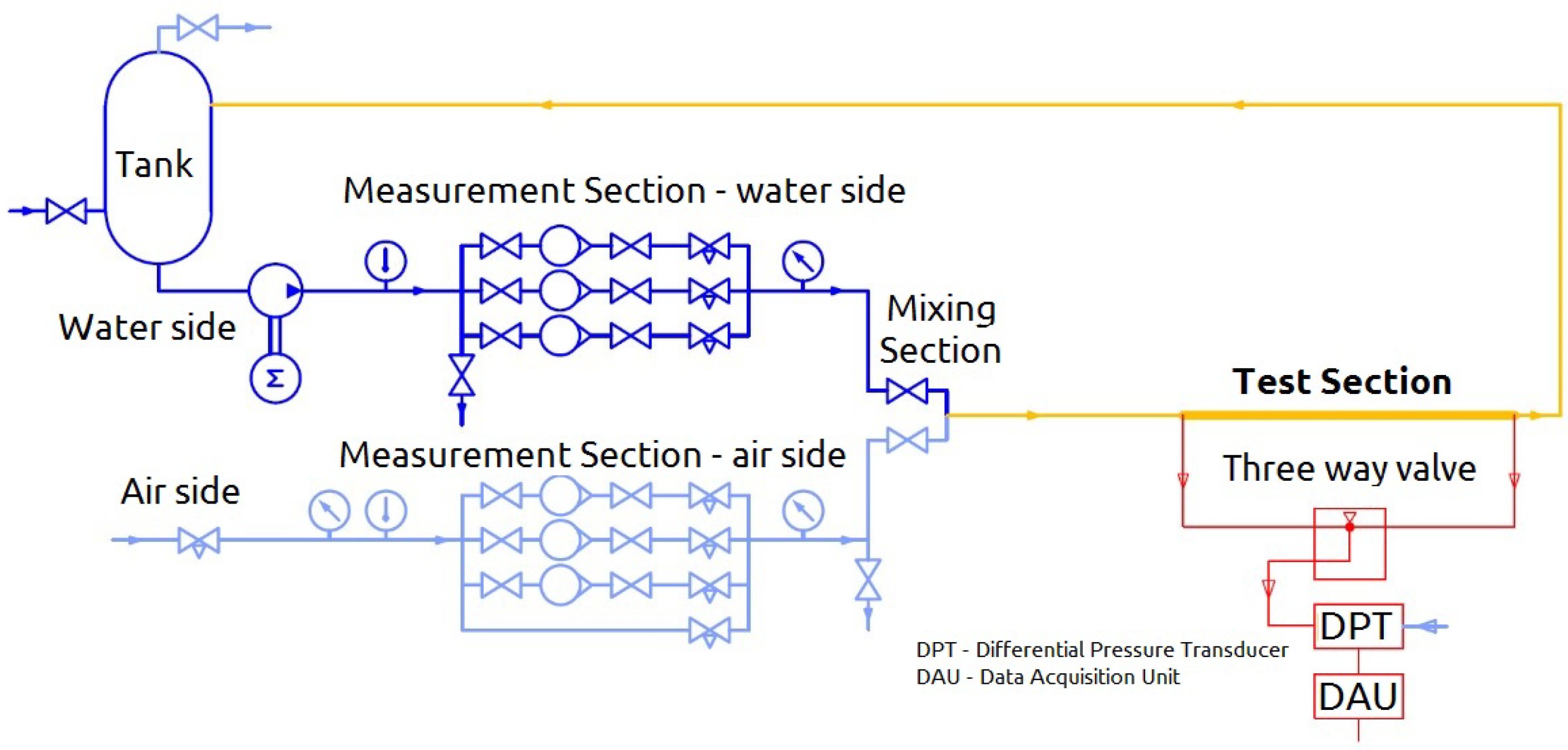
3.1. Overview of the Laboratory Setup

The simplified configuration of the laboratory setup is depicted in Figure 1. Water is pumped from the storage tank, passing through the temperature, pressure, and volume flow rate measurement section, then proceeding to the mixing section and subsequently to the test section. Finally, it flows back to the tank. The volumetric flow rate is assessed using a trio of parallel rotameters, with each specifically designed to accommodate a distinct range of flow rates. Compressed air, provided by the building’s auxiliary supply system, passes through the temperature, pressure, and volumetric flow rate measurement section, proceeds to the mixing section, and finally to the test section. Next, it flows to the tank where, after separation from the water, it is vented to the environment. Similarly, the volumetric flow rate of the air is gauged by a set of three parallel rotameters.
The test section is a copper tube, the properties of which are provided in Table 3. Pressure taps are installed at both the inlet and outlet of the test section, and these taps are connected to a differential pressure transducer (DPT). The DPT then sends electrical signals to a data-acquisition unit (DAU). Each pressure tap is connected to the pressure transducer through a pair of nylon tubes filled with water, enabling the hydraulic transmission of pressure variations. A bypass valve enables measuring either the pressure drop between the two pressure taps or the pressure difference between each tap and the ambient, which is more convenient for reducing the signal-to-noise ratio under specific operating conditions. The data-acquisition unit operates at a sampling frequency of 1 kHz with an acquisition time of 15 s. The maximum measurable pressure difference is about 70 kPa. Table 4 reports the uncertainties of the employed measurement devices. It is noteworthy to emphasize that, given the adiabatic nature of the studied flow in this investigation, temperature measurements are solely utilized in the data processing phase. Consequently, the inherent uncertainty associated with the thermometer has a negligible influence on the final results.
The investigated range of the water and air volume flow rate were 10 to 100 [ Nl h ] with a step of 10 [ Nl h ] and 500 to 4000 [ Nl h ] with a step of 500 [ Nl h ], respectively. The pressure of both water and air in the measurement section was maintained at a constant value of 2.2 [bar] and 3 [bar]. The temperature was measured at the initiation of each test, being insignificantly variable between 22 and 25 °C for water and 19 to 21 °C for air. Starting from the minimum water flow rate, the airflow rate was systematically adjusted to cover the entire range. At each stage, steady-state conditions were achieved through iterative adjustments of the volume flow rates using regulation valves, ensuring constant pressure in the measurement section. Measurements at each step were repeated 5 to 10 times, depending on the observed fluctuations, and averaged as a single data point which resulted in 119 measured data points.

3.2. Data Processing

All of the fluid properties were evaluated at the inlet temperature and at the arithmetic average between the inlet and outlet pressure. The airflow meter readings are calibrated to normal conditions, defined as T 0 = 20 °C and P 0 = 101,325 Pa. According to the manufacturer’s specifications, by taking the actual temperature ( T m s ) and pressure ( p m s ) at the measurement segment and the average pipe pressure ( p a v ) , the actual volume flow rate flowing in the pipe is calculated as
Q = Q 0 p m s p 0 p a v 2 T m s T 0
Consequently, the air superficial velocity in the test section ranges between 5 and 34 [ m s ] . On the other hand, the water superficial velocity varies between 0.05 and 0.45 [ m s ] , which causes the observed flow regimes to vary from wavy to annular flow (at low water velocity) and from slug flow to annular/annular-mist flow, approximately in accordance with the Mandhane map [40]. The pressure drop across the test section was determined from the difference between inlet and outlet measured pressures. With the flow being fully developed, the pressure gradient was determined by calculating the ratio of the pressure drop to the distance between the pressure taps. A summary of the operating conditions are provided with the test section specifications (Table 3).

4. Machine Learning

4.1. Overall Framework

Since, in the present study, the machine learning algorithms are utilized for predicting a known target, which is a continuous value, the overall framework is a supervised regression problem. Accordingly, the machine learning models are employed in order to predict the target value, while being provided a set of features (input parameters). The provided dataset is randomly divided into two subsets: a training subset used to optimize the machine learning algorithms, and a test subset which comprises 20% of the dataset and is utilized to determine the corresponding accuracy. In order to evade the dependence of the determined accuracy on the choice of training and validation subsets, the k-fold cross-validation methodology is employed (with the k = 10). In this procedure, the training is divided into k subsets, and each subset is once used as the validation set, while the remaining subsets are used for the training. In an iterative procedure, all of the subsets will then play the role of the validation set thus predictions, are provided for all of the samples of the training set.
In order to compare the accuracy of different models, several metrics including the Mean Percentage Error (MPE) (Equation (18)), and the Mean Absolute Percentage Error (MAPE) (Equation (19)), were considered. MPE and MAPE were chosen as the primary metrics since the current study aims to compare its achieved performance with the one obtained using existing physical models. As the performance of these physical (empirical) models, in the previous studies, has been reported using MPE and MAPE, for the sake of coherence, these metrics have also been utilized in the present study. Additionally, these metrics are among the most commonly used evaluation metrics in other studies focused on data-driven models in this area, which thus facilitates performing comparisons with previously proposed models. The Mean Absolute Percentage Error (MAPE) is then utilized as the primary accuracy metric for selecting the most promising models.
M P E = 1 N i = 1 N y i , p r e d y i , e x p y i , e x p [ % ]
M A P E = 1 N i = 1 N y i , p r e d y i , e x p y i , e x p [ % ]

4.2. Machine Learning Algorithms

In the present study, the machine learning pipelines have been first developed employing Random Forest [41] as the benchmark algorithm, which is an ensemble method built upon decision trees.

4.3. Optimisation of Machine Learning Pipelines

Following the implementation of machine learning-based pipelines using the selected benchmark algorithms, a genetic algorithm-based optimization procedure is carried out in order to improve the model accuracy by selecting the most effective combination of preprocessing steps and machine learning models with their corresponding optimal hyperparameters.
The optimization procedure is conducted employing TPOT, a Tree-Based Pipeline Optimization Tool [42], while defining a custom objective function that considers MAPE as the key accuracy metric. This AutoML employs various combinations of preprocessing methods, feature selection techniques, and machine learning models to find the best pipeline.

4.3.1. Optimization Settings

The corresponding key settings include the following:
  • Generations (generations = 100): number of iterations for the genetic algorithm.
  • Population Size (population size = 100): number of candidate pipelines in each generation.
  • Scoring Function (MAPE): Mean Absolute Percentage Error used to evaluate pipeline performance.
  • Cross-Validation (cv = 10): 10-fold cross-validation to assess pipeline generalizability.

4.3.2. Pool of Hyperparameters

The hyperparameters search pool includes a variety of preprocessors and machine learning algorithms [43] with their respective hyperparameters such as the depth of decision trees, the number of trees in a Random Forest, regularization parameters in linear models, and learning rates in gradient boosting machines. The major optimized hyperparameters for the considered machine learning algorithms are provided in Table 5.
The pipeline structure optimization enhances the overall pipeline, refining the combination and sequence of preprocessing steps and model training components. Although feature selection methods are included in the optimization process, they are not implemented in this study since a more comprehensive feature selection procedure has been performed in the previous step.

5. Methodology and Implemented Pipelines

Various machine learning-based pipelines are employed to identify the most promising one that yields the most accurate prediction of the pressure drop, given the considered features. In the initial stage, a comprehensive grid search (GridSearchCV [43]) was conducted to determine the optimal Random Forest as the benchmark algorithm by exploring the hyperparameters listed in Table 5. Subsequently, all potential features are fed into the benchmark algorithm, and the corresponding accuracies are recorded. In the next step, the feature selection procedure, explained in the next sub-section, is executed to ascertain the most promising combination of features, employing the benchmark algorithm, resulting in the highest achievable accuracy. Finally, the pipeline optimization procedure, as explained in Section 4.3, considering the selected features as the input is conducted to identify the optimal machine learning algorithm along with their associated tuning parameters.

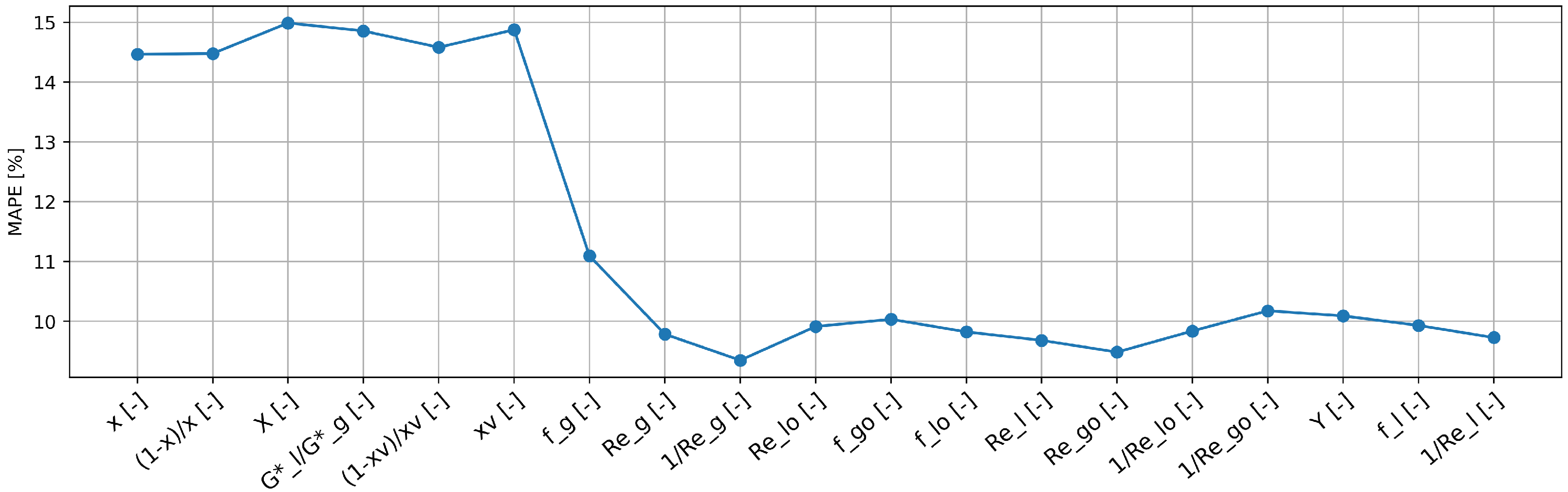
5.1. Feature Selection Procedure

As was previously pointed out, the objective of the feature selection procedure is to determine the most promising set of features that leads to the highest accuracy. An ideal solution to achieve the mentioned goal is evaluating all possible combinations of features, though the latter leads to an excessive computational cost, which makes it practically infeasible. Accordingly, an alternative procedure is implemented, in which the features are first ordered based on their rank ((determined by their Pearson’s correlation coefficient [44] to the target (two-phase pressure drop multipliers)). The features are then added one by one and the resulting set is provided to the machine learning model as input features and the resulting MAPE value at each step is registered. The employed machine learning model in this procedure is Random Forest, which is considered as the key benchmark algorithm for the studied case. The set of features, that results in the lowest MAPE (initial chosen set), is next selected. The remaining features are divided into two categories: the ones that had increased the MAPE, and the ones that had decreased it. The features that had increased the MAPE are discarded, while the ones that had decreased MAPE are sorted in descending order (based on the MAPE achieved while adding them) and added at the beginning of the initial chosen set. The obtained chosen set is again provided to the Random Forest algorithm as the set of features; the features are then dropped one by one, and the resulting MAPE at each step is registered again. The set of features that leads to the lowest possible MAPE value is chosen as the updated set of selected features. Subsequently, the Random Forest is initially fitted with each selected feature individually (as a single input), and the one yielding the lowest Mean Absolute Percentage Error (MAPE) is chosen as the first feature. In the next step, the model is trained utilizing solely two variables (the first one is already chosen), where each of the remained features is given as the second feature. Similarly, the one that leads to the lowest MAPE is chosen as the second feature. This procedure persists until all selected features are incorporated. Evidently, the result obtained in the last step is the same as the one provided in the previous step. The final set of selected features is the one that results in the minimum MAPE value. Finally, it is noteworthy that only the dimensionless numbers that represent the governing phenomena are employed in this work, which results in a rather limited number of features. Thus, executing the proposed gradual selection method results in a limited computational cost. Therefore, taking into account the fact that the feature selection procedure is performed offline (and not in real-time or in-operando), the corresponding execution time does not limit the application of the method in the present work’s context.

5.2. Feature Selection Based on Random Forest-Derived Feature Importance

To compare the effectiveness of the utilized feature selection procedure in the current study, another feature selection approach based on the feature importance of Random Forest algorithm [45] has been applied. The Random Forest algorithm quantifies the significance of a feature by assessing the extent to which the model’s accuracy decreases when that feature is randomly permuted or shuffled while maintaining all other features unchanged [45]. In this approach, features are initially ranked by their importance employing the optimal benchmark. The process begins by using the most important feature for predictions and recording the accuracy achieved. Subsequently, each additional feature is sequentially incorporated, and predictions are made at each step. This iterative process continues until all features have been included. The elbow method is then applied to determine the optimal set of features. Finally, the performance of the model using this optimal feature set is evaluated on both the training/validation set and the test set, and the results are reported accordingly.

6. Results and Discussions

6.1. Accuracy of Existing Standard Physical Models

The accuracies of pressure gradient prediction from various models for the two-phase dataset are presented in Table 6. The model proposed by Muller-Steinhagen and Heck [16] is identified as the most accurate, resulting in a Mean Absolute Percentage Error (MAPE) of 15.79%.

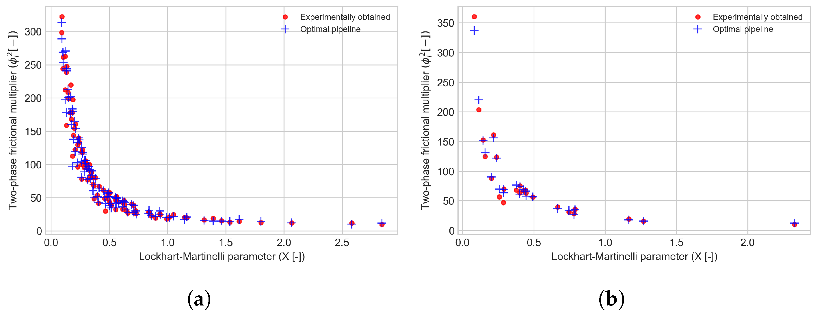
6.2. Implemented Hybrid Data-Driven/Physical-Based Models

As was previously mentioned, two-phase flow multipliers are taken into account as targets, while the non-dimensional parameters are given as inputs. Consequently, four general machine learning-based pipelines were defined, in which the target wasn defined as a liquid, liquid only, gas, or gas-only multiplier. For each of the above-mentioned targets, the Random Forest-based pipelines were first implemented both with all features and selected features. Next, the optimal pipeline, given the selected features, was determined for each scenario, and the resulting accuracies were compared.
Table 7 represents the prediction accuracies that are obtained while employing the abovementioned pipelines. The most accurate optimal pipeline was determined to be the one with the Φ l 2 as the target and utilizing selected features which leads to an MAPE of 5.99% on the validation set and 7.03% on the test set.
The comprehensive grid search was conducted for each target employing all the input features (Table 8). The optimal benchmark algorithm for Φ l 2 is defined as described in Table A1. Table 8, in addition to the list of all of the input features, provides their corresponding Pearson correlation with respect to the targets. These correlations are used initially to rank the features in the feature selection step. The feature selection results in Table 9 demonstrate that the model requires only three input parameters (x, R e g , and X), significantly simplifying it with respect to physical models. Clearly, the reason behind the fact that only three parameters are selected is that only one pair of fluids (water and air) is utilized in this study; accordingly, the other parameters that depend on the material properties do not provide additional information.
Next, the performance of the three-step feature selection performed was compared with the methodology provided in Section 5.2. The accuracy obtained by progressively adding features, based on their importance as determined by the Random Forest algorithm, is depicted in Figure 2. It can be observed that by expanding the list of input features, improvements in results are obtained up to a certain point. The plot illustrates that improvements in results are observed as more input features are included, reaching an optimal point. Using the elbow method, the optimal set of features, consisting of nine features, is identified. Finally, the identified set of features is used to make predictions on both the training/validation and test sets, resulting in accuracies of 9.35% and 15.70% in terms of MAPE, respectively. It is evident that the three-step feature selection method employed in this study (pipeline B) outperforms the feature importance-driven method, achieving higher prediction accuracies with only three selected features.
Next, the details of the optimal pipeline identified in the current work are provided. Figure 3 provides the ML algorithms of the optimized pipeline and the corresponding additional feature processing. Additionally, Table A2 in Appendix A section provides the attributes and the detailed description of each parameter utilized in the various steps of the optimal pipeline.
Figure 4 compares the estimated two-phase multiplier values generated by this pipeline and the corresponding experimental data, with respect to the Lockhart–Martinelli parameter X [-].
Figure 5 illustrates the comparison between the measured pressure gradient values, those estimated by Muller-Steinhagen and Heck [16], and the predictions of the proposed optimal pipeline. Using the obtained Φ l o 2 and employing Equation (6) the pressure gradient values were calculated (as mentioned in Section 6.1) and are compared to experimental data. It can be observed that the model proposed by Muller-Steinhagen and Heck [16] overestimates the low-pressure gradient ranges and underestimates high-pressure gradient values. Additionally, it can be noted that the optimal model demonstrates a significantly higher accuracy in estimating the two-phase pressure drop compared to the Muller-Steinhagen and Heck [16], which is the most precise physical model currently available in the literature.
Furthermore, since both the dataset and the optimal pipeline are made publicly accessible as tools, the latter approach also enhances reproducibility and ease of use.

7. Conclusions

In the present study, an experimental study was first conducted in which the frictional pressure drop of the water–air mixture (two-phase), while passing through a smooth horizontal tube at various flow conditions was measured. In the next step, on the acquired dataset, the state-of-the-art standard physical models, proposed in the literature, were applied and the corresponding accuracy, being implemented to the experimentally acquired dataset, was calculated and the most accurate models were determined. Next, machine learning-based pipelines, while following dimensionless approaches, were implemented. In this approach, the two-phase flow multipliers were employed as the targets while only non-dimensional parameters were employed as features. Feature selection and pipeline optimization procedures were applied to each pipeline in order to determine the most promising set of features along with the most accurate machine learning algorithm (and the associated tuning parameters), respectively. The optimal pipeline was determined to be the one where the liquid two-phase multiplier serves as the target, and three dimensionless parameters (chosen from 19 provided features) are utilized as input features. Employing the latter pipeline, a MAPE of 5.99% on the validation set and 7.03% on the test set can be achieved that is notably more accurate than the most promising physical model (Muller-Steinhagen and Heck [16] leading to a MAPE of 15.79% on the whole dataset). It can be mentioned that other methods such as Bayesian optimization are also available for pipeline optimization, and while AutoML methods that are based on Bayesian optimization methods, such as those implemented in tools like auto-sklearn [46], offer advantages in certain aspects, including efficient handling of continuous parameters and better performance with limited data, they may not always outperform genetic algorithms in terms of scalability and ability to handle diverse types of hyper-parameters. However, there are Bayesian optimization methods designed for scalability and handling mixed variables, thus eliminating the need for the extensive evaluations required by genetic algorithms. Therefore, it is recommended for future work to explore Bayesian optimization methods for optimizing machine learning-based pipelines in predicting pressure drops in smooth tubes. This approach could significantly enhance the efficiency and accuracy of the optimization process.
The feature selection procedure provided in the current work effectively assessed the performance of various combinations of input features in predicting the pressure drop, allowing for the identification of the most promising set. This study demonstrated that a significant reduction in the number of input parameters can be achieved while maintaining accuracy, thereby enhancing the interpretability of the results. Nevertheless, other methods regarding explainable machine learning such as the Sindys [47,48] via Neural Networks can be employed to achieve/enhance the explainability of the model in future works. Finally, with the public accessibility of both the dataset and the optimal pipelines, the proposed model offers superior reproducibility and user-friendliness compared to state-of-the-art physical models.

Author Contributions

F.B.: Software, Formal analysis, Methodology, Validation, Data Curation, Writing—Original Draft; K.A.: Formal analysis, Methodology, Validation, Data Curation, Writing—Original Draft; F.D.J.: Software, Data Curation, Writing—Original Draft; B.N.: Conceptualization, Methodology, Supervision, Writing—Review & Editing; P.V.P.D.: Validation, Data Curation; F.R.: Supervision, Funding acquisition; L.P.M.C.: Supervision, Conceptualization, Methodology. All authors have read and agreed to the published version of the manuscript.

Funding

This research received no external funding.

Data Availability Statement

The processed dataset and the resulting optimal pipelines, including the most promising feature sets and the most suitable algorithms, are available in an online repository: https://github.com/FarzadJavan/Pressure-Drop-Estimation-of-Two-Phase-Adiabatic-Flows-in-Smooth-Tubes (accessed on 12 June 2024).

Conflicts of Interest

The authors declare that they have no known competing financial interests or personal relationships that could have appeared to influence the work reported in this paper.

Nomenclature

Δ p Pressure drop [Pa]
Δ p Δ z Pressure gradient [ Pa m ]
N l h Normal litter per hour
A I Artificial intelligence
A N N Artificial Neural Network
C V Cross-Validation
D i n t Pipe internal diameter [m]
fFriction factor (by Fanning) [-]
F r Froude number [-]
GMass flux [ kg m 2 s ]
G * Apparent mass flux [ kg m 2 s ]
JSuperficial velocity m s
L a Laplace constant [-]
M A P E Mean Absolute Percentage Error [%]
M L Machine learning
M P E Mean Percentage Error [%]
pPressure [Pa]
QVolume flow rate [ m 3 s ]
R e Reynolds number [-]
R F Random Forest algorithm
SInternal wetted perimeter [m]
S V M Support Vector Machines
UPhase velocity m s
W e Weber number [-]
XLockhart–Martinelli parameter [-]
xAverage mass quality [-]
x v Average volume quality [-]
YChisholm parameter [-]
Greek symbols
α Void fraction [-]
Γ Mass flow rate [ kg s ] , non-dimensional parameter (Equation (13))
μ Dynamic viscosity [ Pa s ]
Ω Cross-section [ m 2 ]
Φ 2 Two-phase flow friction multiplier [-]
ρ Density [ kg m 3 ]
σ Surface tension [ N m ]
τ w Shear stress [Pa]
Subscripts
aAccelerative
a v Average
bBulk
e x p Experimental value
fFrictional
g o Gas only
lLiquid
l o Liquid only
mMicro-finned
m s Manufacturer’s specifications
p r e d Predicted value
sSmooth
t p Two-phase
t t Turbulent liquid, turbulent gas flow
t v Turbulent liquid, laminar gas flow
v t Laminar liquid, turbulent gas flow
v v Laminar liquid, Laminar gas flow

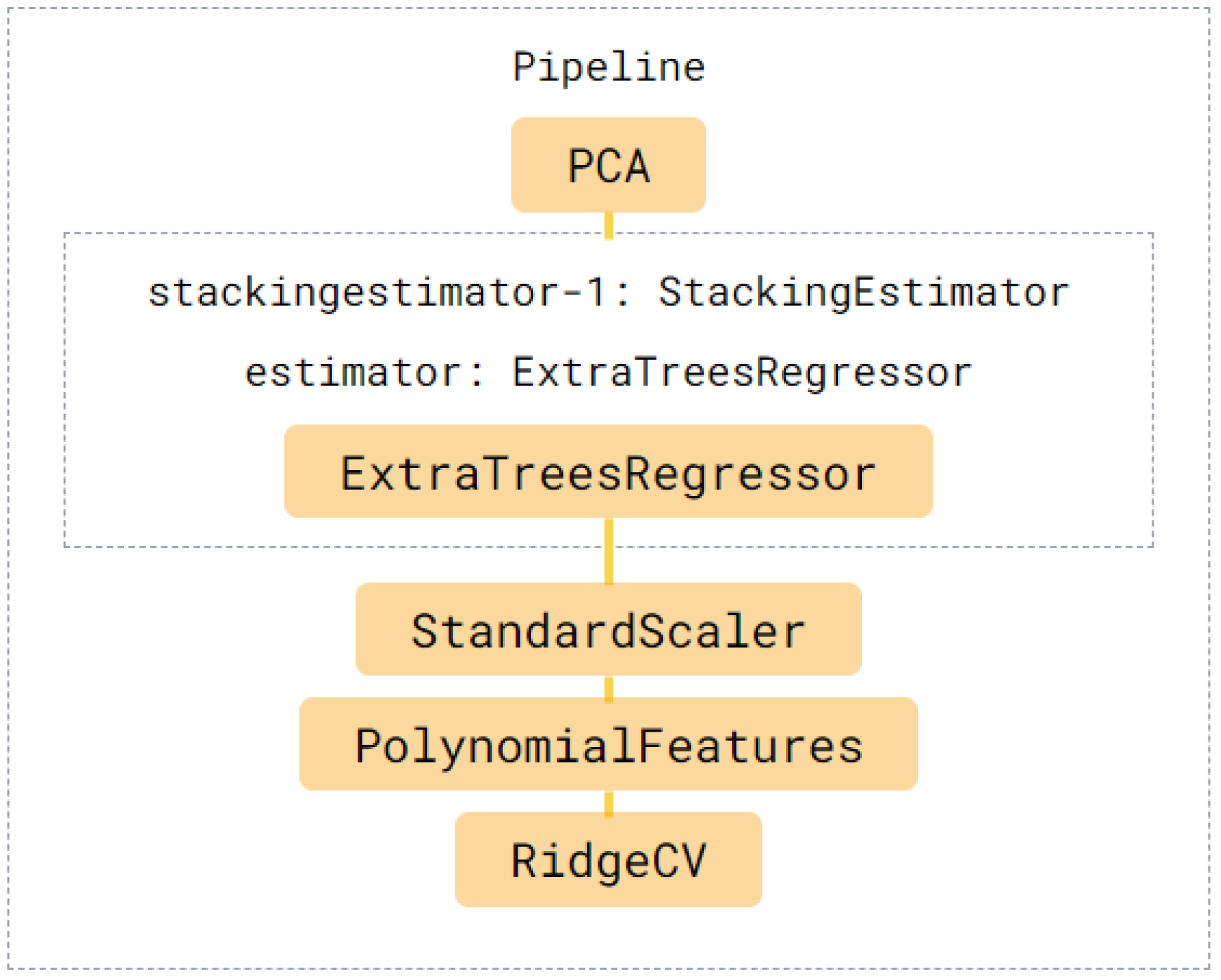
Appendix A. Optimal Pipeline

Table A1. Attributes of the identified optimal Random Forest (pipelines A and B) along with the description of each parameter (defined by scikit-learn guidelines [43]).
Optimal Benchmark AlgorithmArgumentsDefinitionsValues
RandomForestRegressorbootstrapWhether bootstrap samples are used
when building trees
False
max-featuresThe number of features to consider
when looking for the best split
0.2
min-samples-leafThe minimum number of samples
required to be at a leaf n
1
min-samples-splitThe minimum number of samples
required to split an internal node
2
n-estimatorsThe number of trees in the forest100
Table A2. Attributes of the identified optimal pipeline (Pipeline C) along with the description of each parameter (defined by scikit-learn guidelines [43]).
Optimal Pipeline StepsArgumentsDefinitionsValues
Step 1: PCA 1iterated-powerThe number of iterations used by the
randomized SVD solver to improve accuracy
3
svd-solverSelects the algorithm for computing SVD,
balancing speed and accuracy
randomized
Step 2: StackingEstimator:
estimator = ExtraTreesRegressor
bootstrapWhether bootstrap samples are used
when building trees
False
max-featuresThe number of features to consider
when looking for the best split
0.95
min-samples-leafThe minimum number of samples
required to be at a leaf n
15
min-samples-splitThe minimum number of samples
required to split an internal node
8
n-estimatorsThe number of trees in the forest100
Step 3: StandardScaler 2---
Step 4: PolynomialFeatures 3degreeThe degree of the polynomial features2
include-biasbias column is consideredFalse
interaction-onlyinteraction features are producedFalse
Step 5: RidgeCV---
1 A pre-processing step that reduces dimensionality by transforming data into a set of orthogonal principal components that capture the maximum variance. 2 A pre-processing step that standardizes features by removing the mean and scaling them to unit variance. 3 A pre-processing step that generates a new feature matrix consisting of all polynomial combinations of the features with degree less than or equal to the specified degree.

References

  1. Szilas, A.P. Production and Transport of Oil and Gas; Elsevier: Amsterdam, The Netherlands, 2010. [Google Scholar]
  2. Ebrahimi, A.; Khamehchi, E. A robust model for computing pressure drop in vertical multiphase flow. J. Nat. Gas Sci. Eng. 2015, 26, 1306–1316. [Google Scholar] [CrossRef]
  3. Osman, E.S.A.; Aggour, M.A. Artificial neural network model for accurate prediction of pressure drop in horizontal and near-horizontal-multiphase flow. Pet. Sci. Technol. 2002, 20, 1–15. [Google Scholar] [CrossRef]
  4. Taccani, R.; Maggiore, G.; Micheli, D. Development of a process simulation model for the analysis of the loading and unloading system of a CNG carrier equipped with novel lightweight pressure cylinders. Appl. Sci. 2020, 10, 7555. [Google Scholar] [CrossRef]
  5. Xu, Y.; Fang, X. A new correlation of two-phase frictional pressure drop for evaporating flow in pipes. Int. J. Refrig. 2012, 35, 2039–2050. [Google Scholar] [CrossRef]
  6. Xu, Y.; Fang, X.; Su, X.; Zhou, Z.; Chen, W. Evaluation of frictional pressure drop correlations for two-phase flow in pipes. Nucl. Eng. Des. 2012, 253, 86–97. [Google Scholar] [CrossRef]
  7. Lockhart, R.; Martinelli, R. Proposed correlation of data for isothermal two-phase, two-component flow in pipes. Chem. Eng. Prog. 1949, 45, 39–48. [Google Scholar]
  8. Chisholm, D. A theoretical basis for the Lockhart-Martinelli correlation for two-phase flow. Int. J. Heat Mass Transf. 1967, 10, 1767–1778. [Google Scholar] [CrossRef]
  9. Mishima, K.; Hibiki, T. Some characteristics of air-water two-phase flow in small diameter vertical tubes. Int. J. Multiph. Flow 1996, 22, 703–712. [Google Scholar] [CrossRef]
  10. Zhang, W.; Hibiki, T.; Mishima, K. Correlations of two-phase frictional pressure drop and void fraction in mini-channel. Int. J. Heat Mass Transf. 2010, 53, 453–465. [Google Scholar] [CrossRef]
  11. Sun, L.; Mishima, K. Evaluation analysis of prediction methods for two-phase flow pressure drop in mini-channels. In Proceedings of the International Conference on Nuclear Engineering, Orlando, FL, USA, 11–15 May 2008; Volume 48159, pp. 649–658. [Google Scholar]
  12. Colombo, M.; Colombo, L.P.; Cammi, A.; Ricotti, M.E. A scheme of correlation for frictional pressure drop in steam–water two-phase flow in helicoidal tubes. Chem. Eng. Sci. 2015, 123, 460–473. [Google Scholar] [CrossRef]
  13. De Amicis, J.; Cammi, A.; Colombo, L.P.; Colombo, M.; Ricotti, M.E. Experimental and numerical study of the laminar flow in helically coiled pipes. Prog. Nucl. Energy 2014, 76, 206–215. [Google Scholar] [CrossRef]
  14. Chisholm, D. Pressure gradients due to friction during the flow of evaporating two-phase mixtures in smooth tubes and channels. Int. J. Heat Mass Transf. 1973, 16, 347–358. [Google Scholar] [CrossRef]
  15. Baroczy, C. Systematic Correlation for Two-Phase Pressure Drop. Chem. Eng. Progr. Symp. Ser. 1966, 62, 232–249. [Google Scholar]
  16. Müller-Steinhagen, H.; Heck, K. A simple friction pressure drop correlation for two-phase flow in pipes. Chem. Eng. Process. Process. Intensif. 1986, 20, 297–308. [Google Scholar] [CrossRef]
  17. Lobo de Souza, A.; de Mattos Pimenta, M. Prediction of pressure drop during horizontal two-phase flow of pure and mixed refrigerants. ASME-Publ.-FED 1995, 210, 161–172. [Google Scholar]
  18. Friedel, L. Improved friction pressure drop correlation for horizontal and vertical two-phase pipe flow. In Proceedings of the European Two-Phase Group Meeting, Ispra, Italy, 5–8 June 1979. [Google Scholar]
  19. Cavallini, A.; Censi, G.; Del Col, D.; Doretti, L.; Longo, G.A.; Rossetto, L. Condensation of halogenated refrigerants inside smooth tubes. Hvac&R Res. 2002, 8, 429–451. [Google Scholar]
  20. Tran, T.; Chyu, M.C.; Wambsganss, M.; France, D. Two-phase pressure drop of refrigerants during flow boiling in small channels: An experimental investigation and correlation development. Int. J. Multiph. Flow 2000, 26, 1739–1754. [Google Scholar] [CrossRef]
  21. Najafi, B.; Ardam, K.; Hanušovský, A.; Rinaldi, F.; Colombo, L.P.M. Machine learning based models for pressure drop estimation of two-phase adiabatic air-water flow in micro-finned tubes: Determination of the most promising dimensionless feature set. Chem. Eng. Res. Des. 2021, 167, 252–267. [Google Scholar] [CrossRef]
  22. Ardam, K.; Najafi, B.; Lucchini, A.; Rinaldi, F.; Colombo, L.P.M. Machine learning based pressure drop estimation of evaporating R134a flow in micro-fin tubes: Investigation of the optimal dimensionless feature set. Int. J. Refrig. 2021, 131, 20–32. [Google Scholar] [CrossRef]
  23. Bar, N.; Bandyopadhyay, T.K.; Biswas, M.N.; Das, S.K. Prediction of pressure drop using artificial neural network for non-Newtonian liquid flow through piping components. J. Pet. Sci. Eng. 2010, 71, 187–194. [Google Scholar] [CrossRef]
  24. Tian, Z.; Gu, B.; Yang, L.; Liu, F. Performance prediction for a parallel flow condenser based on artificial neural network. Appl. Therm. Eng. 2014, 63, 459–467. [Google Scholar] [CrossRef]
  25. Garcia, J.J.; Garcia, F.; Bermúdez, J.; Machado, L. Prediction of pressure drop during evaporation of R407C in horizontal tubes using artificial neural networks. Int. J. Refrig. 2018, 85, 292–302. [Google Scholar] [CrossRef]
  26. López-Belchí, A.; Illan-Gomez, F.; Cano-Izquierdo, J.M.; García-Cascales, J.R. GMDH ANN to optimise model development: Prediction of the pressure drop and the heat transfer coefficient during condensation within mini-channels. Appl. Therm. Eng. 2018, 144, 321–330. [Google Scholar] [CrossRef]
  27. Khosravi, A.; Pabon, J.; Koury, R.; Machado, L. Using machine learning algorithms to predict the pressure drop during evaporation of R407C. Appl. Therm. Eng. 2018, 133, 361–370. [Google Scholar] [CrossRef]
  28. Zendehboudi, A.; Li, X. A robust predictive technique for the pressure drop during condensation in inclined smooth tubes. Int. Commun. Heat Mass Transf. 2017, 86, 166–173. [Google Scholar] [CrossRef]
  29. Shadloo, M.S.; Rahmat, A.; Karimipour, A.; Wongwises, S. Estimation of Pressure Drop of Two-Phase Flow in Horizontal Long Pipes Using Artificial Neural Networks. J. Energy Resour. Technol. 2020, 142, 112110. [Google Scholar] [CrossRef]
  30. Yan, Y.; Wang, L.; Wang, T.; Wang, X.; Hu, Y.; Duan, Q. Application of soft computing techniques to multiphase flow measurement: A review. Flow Meas. Instrum. 2018, 60, 30–43. [Google Scholar] [CrossRef]
  31. Shaban, H.; Tavoularis, S. Measurement of gas and liquid flow rates in two-phase pipe flows by the application of machine learning techniques to differential pressure signals. Int. J. Multiph. Flow 2014, 67, 106–117. [Google Scholar] [CrossRef]
  32. Nie, F.; Yan, S.; Wang, H.; Zhao, C.; Zhao, Y.; Gong, M. A universal correlation for predicting two-phase frictional pressure drop in horizontal tubes based on machine learning. Int. J. Multiph. Flow 2023, 160, 104377. [Google Scholar] [CrossRef]
  33. Faraji, F.; Santim, C.; Chong, P.L.; Hamad, F. Two-phase flow pressure drop modelling in horizontal pipes with different diameters. Nucl. Eng. Des. 2022, 395, 111863. [Google Scholar] [CrossRef]
  34. Moradkhani, M.; Hosseini, S.; Song, M.; Abbaszadeh, A. Reliable smart models for estimating frictional pressure drop in two-phase condensation through smooth channels of varying sizes. Sci. Rep. 2024, 14, 10515. [Google Scholar] [CrossRef] [PubMed]
  35. Moradkhani, M.; Hosseini, S.H.; Mansouri, M.; Ahmadi, G.; Song, M. Robust and universal predictive models for frictional pressure drop during two-phase flow in smooth helically coiled tube heat exchangers. Sci. Rep. 2021, 11, 20068. [Google Scholar] [CrossRef] [PubMed]
  36. McAdams, W. Vaporization inside horizontal tubes-II, Benzene oil mixtures. Trans. ASME 1942, 64, 193–200. [Google Scholar] [CrossRef]
  37. Beattie, D.; Whalley, P. A simple two-phase frictional pressure drop calculation method. Int. J. Multiph. Flow 1982, 8, 83–87. [Google Scholar] [CrossRef]
  38. Awad, M.; Muzychka, Y. Effective property models for homogeneous two-phase flows. Exp. Therm. Fluid Sci. 2008, 33, 106–113. [Google Scholar] [CrossRef]
  39. Vega-Penichet Domecq, P. Pressure Drop Measurement for Adiabatic Single and Two Phase Flows inside Horizontal Micro-Fin Tubes. Available online: https://oa.upm.es/52749/ (accessed on 12 June 2024).
  40. Mandhane, J.; Gregory, G.; Aziz, K. A flow pattern map for gas–liquid flow in horizontal pipes. Int. J. Multiph. Flow 1974, 1, 537–553. [Google Scholar] [CrossRef]
  41. Breirnan, L. Arcing classifiers. Ann. Stat. 1998, 26, 801–849. [Google Scholar]
  42. Olson, R.S.; Bartley, N.; Urbanowicz, R.J.; Moore, J.H. Evaluation of a tree-based pipeline optimization tool for automating data science. In Proceedings of the Genetic and Evolutionary Computation Conference 2016, Denver, CO, USA, 20–24 July 2016; pp. 485–492. [Google Scholar]
  43. Pedregosa, F.; Varoquaux, G.; Gramfort, A.; Michel, V.; Thirion, B.; Grisel, O.; Blondel, M.; Prettenhofer, P.; Weiss, R.; Dubourg, V.; et al. Scikit-learn: Machine learning in Python. J. Mach. Learn. Res. 2011, 12, 2825–2830. [Google Scholar]
  44. Pearson, K. VII. Note on regression and inheritance in the case of two parents. Proc. R. Soc. Lond. 1895, 58, 240–242. [Google Scholar]
  45. Breiman, L. Random forests. Mach. Learn. 2001, 45, 5–32. [Google Scholar] [CrossRef]
  46. Feurer, M.; Klein, A.; Eggensperger, K.; Springenberg, J.; Blum, M.; Hutter, F. Efficient and robust automated machine learning. Adv. Neural Inf. Process. Syst. 2015, 28. Available online: https://proceedings.neurips.cc/paper/2015/hash/11d0e6287202fced83f79975ec59a3a6-Abstract.html (accessed on 12 June 2024).
  47. Brunton, S.L.; Proctor, J.L.; Kutz, J.N. Discovering governing equations from data by sparse identification of nonlinear dynamical systems. Proc. Natl. Acad. Sci. USA 2016, 113, 3932–3937. [Google Scholar] [CrossRef] [PubMed]
  48. Loiseau, J.C.; Brunton, S.L. Constrained sparse Galerkin regression. J. Fluid Mech. 2018, 838, 42–67. [Google Scholar] [CrossRef]
Figure 1. A schematic depiction illustrating the laboratory configuration employed for conducting the experimental procedures.
Fluids 09 00181 g001
Figure 2. Obtained accuracy by progressively adding features based on Random Forest algorithm-derived importance, focusing on ϕ l 2 as the target.
Fluids 09 00181 g002
Figure 3. A schematic description of the identified optimal pipeline (Pipeline C).
Fluids 09 00181 g003
Figure 4. Comparison between the experimentally obtained two-phase flow multiplier and the estimation by the optimal pipeline (Pipeline C) with respect to the Lockhart–Martinelli parameter X. (a) Training set (CV). (b) Test set.
Fluids 09 00181 g004
Figure 5. Experimentally acquired pressure gradient vs. the optimal pipeline estimations (Pipeline C) and juxtaposed with the values estimated by Muller-Steinhagen and Heck [16] model. (a) Training set (CV). (b) Test set.
Fluids 09 00181 g005
Table 1. Selected models, proposed in the literature, which have utilized the homogeneous approach.
Author(s) and the Respective Reference(s)EquationEq. No
McAdams et al. [36] 1 μ t p = x μ g + 1 x μ l (3)
Beattie and Whalley [37] μ t p = μ l ( 1 β ) ( 1 + 2.5 β ) + μ g β
β = x x + ( 1 x ) ρ g ρ l
(4)
Awad and Muzychka [38] μ t p = μ g 2 μ g + μ l 2 ( μ g μ l ) ( 1 x ) 2 μ g + μ l + ( μ g μ l ) ( 1 x ) (5)
Table 2. Selected models that have employed the separated flow approach.
Author(s) and the Respective Reference(s)EquationEq. No
Chisholm [8] Φ l 2 = 1 + C X + 1 X 2
X 2 = ( Δ p Δ z ) l ( Δ p Δ z ) g
C = 5 for v v , C = 10 for t v
C = 12 for v t , C = 20 for t t
(7)
Mishima and Hibiki [9] C = 21 [ 1 exp ( 0.319 D i n t ) ] (8)
Zhang et al. [10] C = 21 [ 1 exp ( a L a ) ]
L a = σ g ( ρ l ρ g ) D i n t
For gas and liquid a = 0.647
For vapor and liquid a = 0.142
(9)
Sun and Mishima [11]For viscous flow:
C = 26 ( 1 + R e l 1000 ) 1 exp ( 0.153 0.8 + 0.27 L a )
For turbulent flow:
Φ l 2 = 1 + C X 1.19 + 1 X 2
C = 1.79 ( R e g R e l ) 0.4 1 x x
where R e g = G t p x D i n t μ g ,
R e l = G t p ( 1 x ) D i n t μ l
(10)
Chisholm [14] Φ l o 2 = 1 + ( Y 2 1 ) { B [ x ( 1 x ) ] 0.875 + x 1.75 }
Y 2 = ( Δ p Δ z ) g o ( Δ p Δ z ) l o
if 0 < Y < 9.5 , B = 4.8 G t p 500 2400 500 < G t p < 1900 55 G t p 0.5 G t p 1900
if 9.5 < Y < 28 , B = 520 Y G t p 0.5 G t p 600 21 Y G t p > 600
if Y > 28 , B = 15000 Y 2 G t p 0.5
(11)
Muller-Steinhagen and Heck [16] Φ l o 2 = Y 2 x 3 + ( 1 x ) 0.333 [ 1 + 2 x ( Y 2 1 ) ] (12)
Souza and Pimenta [17] Φ l o 2 = 1 + ( Γ 2 1 ) x 1.75 ( 1 + 0.9524 Γ X t t 0.4126 )
Γ = ( ρ l ρ g ) 0.5 ( μ g μ l ) 0.125 ,   X t t = 1 Γ ( 1 x x ) 0.875
(13)
Friedel [18] Φ l o 2 = ( 1 x ) 2 + x 2 ρ l f g o ρ g f l o + 3.24 x 0.78 ( 1 x ) 0.224 H F r t p 0.045 W e t p 0.035
H = ( ρ l ρ g ) 0.91 ( μ g μ l ) 0.19 ( 1 μ g μ l ) 0.7
W e t p = G t p 2 D i n t σ ρ t p ,   F r t p = G t p 2 g D i n t ρ t p 2 ,   1 ρ t p = x ρ g + 1 x ρ l
(14)
Cavallini et al. [19] Φ l o 2 = ( 1 x ) 2 + x 2 ρ l f g o ρ g f l o + 1.262 x 0.6987 H W e g o 0.1458
H = ( ρ l ρ g ) 0.3278 ( μ g μ l ) 1.181 ( 1 μ g μ l ) 3.477
W e g o = G t p 2 D i n t σ ρ g ,
(15)
Tran et al. [20] Φ l o 2 = 1 + ( 4.3 Y 2 1 ) { [ x ( 1 x ) ] 0.875 L a + x 1.75 } (16)
Table 3. Specification of the test section and experimental setup conditions of the flow.
ParametersUnitsValues
Utility-E-C-A
External diameter of the tube[mm]9.52
Thickness of the tube[mm]0.3
Internal diameter of the tube[mm]8.92
Length of the test section[m]1.295
Wet perimeter[mm]28.02
Cross-section area[mm2]62.49
Number of two-phase data points-119
Mass fluxes range of the air [ kg ( m 2 s ) ] 5.30–47.42
Mass fluxes range of the water [ kg ( m 2 s ) ] 44.29–442.91
Mass quality range [ ] 0.01–0.52
Pressure gradient range [ Pa m ] 450.05–20,047.16
Table 4. Specifications of the employed measurement devices.
DeviceRangeUncertainty
Manometer0–6 bar (gauge)0.2 bar
Thermometer5–120 [°C]1 [°C]
Differential Pressure Transducer0–70 kPa1.5% full scale
Air Flow Meter4–190 Nl h 3% of the observed value
Air Flow Meter85–850 Nl h 3% of the observed value
Air Flow Meter400–4000 Nl h 3% of the observed value
Water Flow Meter10–100 Nl h 3% of the observed value
Water Flow Meter40–400 Nl h 3% of the observed value
Table 5. Algorithm search pool and their corresponding hyperparameter range.
ModelHyperparameters
ElasticNetCV
• 
l1_ratio: { 0.0 , 0.05 , 0.1 , , 1.0 }
• 
tol: { 1 × 10 5 , 1 × 10 4 , 1 × 10 3 , 1 × 10 2 , 1 × 10 1 }
ExtraTreesRegressor
• 
n_estimators: 100
• 
max_features: { 0.05 , 0.1 , , 1.0 }
• 
min_samples_split: { 2 , 3 , , 20 }
• 
min_samples_leaf: { 1 , 2 , , 20 }
• 
bootstrap: True or False
GradientBoostingRegressor
• 
n_estimators: 100
• 
loss: {“ls”, “lad”, “huber”, “quantile”}
• 
learning_rate: { 0.001 , 0.01 , 0.1 , 0.5 , 1.0 }
• 
max_depth: { 1 , 2 , , 10 }
• 
min_samples_split: { 2 , 3 , , 20 }
• 
min_samples_leaf: { 1 , 2 , , 20 }
• 
subsample: { 0.05 , 0.1 , , 1.0 }
• 
max_features: { 0.05 , 0.1 , , 1.0 }
• 
alpha: { 0.75 , 0.8 , 0.85 , 0.9 , 0.95 , 0.99 }
AdaBoostRegressor
• 
n_estimators: 100
• 
learning_rate: { 0.001 , 0.01 , 0.1 , 0.5 , 1.0 }
• 
loss: {“linear”, “square”, “exponential”}
DecisionTreeRegressor
• 
max_depth: { 1 , 2 , , 10 }
• 
min_samples_split: { 2 , 3 , , 20 }
• 
min_samples_leaf: { 1 , 2 , , 20 }
KNeighborsRegressor
• 
n_neighbors: { 1 , 2 , , 100 }
• 
weights: {“uniform”, “distance”}
• 
p: { 1 , 2 }
LassoLarsCV
• 
normalize: True or False
LinearSVR
• 
loss: {“squared_epsilon_insensitive”, “epsilon_insensitive”}
• 
dual: True or False
• 
tol: { 1 × 10 5 , 1 × 10 4 , 1 × 10 3 , 1 × 10 2 , 1 × 10 1 }
• 
C: { 1 × 10 4 , . . . , 1 × 10 1 , 0.5 , 1.0 , 5.0 , 10.0 , 15.0 , 20.0 , 25.0 }
• 
epsilon: { 1 × 10 4 , 1 × 10 3 , 1 × 10 2 , 1 × 10 1 , 1.0 }
RandomForestRegressor
• 
n_estimators: 100
• 
max_features: { 0.05 , 0.1 , , 1.0 }
• 
min_samples_split: { 2 , 3 , , 20 }
• 
min_samples_leaf: { 1 , 2 , , 20 }
• 
bootstrap: True or False
XGBRegressor
• 
n_estimators: 100
• 
max_depth: { 1 , 2 , , 10 }
• 
learning_rate: { 0.001 , 0.01 , 0.1 , 0.5 , 1.0 }
• 
subsample: { 0.05 , 0.1 , , 1.0 }
• 
min_child_weight: { 1 , 2 , , 20 }
• 
nthread: 1
• 
objective: {“reg:squarederror”}
SGDRegressor
• 
loss: {“epsilon_insensitive”, “squared_loss”, “huber”}
• 
penalty: {“elasticnet”}
• 
alpha: { 0.0 , 0.01 , 0.001 }
• 
learning_rate: {“invscaling”, “constant”}
• 
fit_intercept: True or False
• 
l1_ratio: { 0.25 , 0.0 , 1.0 , 0.75 , 0.5 }
• 
eta0: { 0.1 , 1.0 , 0.01 }
• 
power_t: { 0.5 , 0.0 , 1.0 , 0.1 , 100.0 , 10.0 , 50.0 }
RidgeCV
Preprocessors
ModelHyperparameters
Binarizer
• 
threshold set to { 0.0 , 0.05 , 0.1 , , 1.0 }
FastICA
• 
tol set to { 0.0 , 0.05 , 0.1 , , 1.0 }
FeatureAgglomeration
• 
linkage set to {“ward”, “complete”, “average”}
• 
affinity set to {“euclidean”, “l1”, “l2”, “manhattan”, “cosine”}
MaxAbsScaler
MinMaxScaler
Normalizer
• 
norm set to {“l1”, “l2”, “max”}
Nystroem
• 
kernel set to {“rbf”, “cosine”, “chi2”, “laplacian”, “polynomial”, “poly”, “linear”, “additive_chi2”, “sigmoid”}
• 
gamma set to { 0.0 , 0.05 , 0.1 , , 1.0 }
• 
n_components set to { 1 , 2 , , 10 }
PCA
• 
svd_solver set to {“randomized”}
• 
iterated_power set to { 1 , 2 , , 10 }
PolynomialFeatures
• 
degree set to 2
• 
include_bias set to False
• 
interaction_only set to False
RBFSampler
• 
gamma set to { 0.0 , 0.05 , 0.1 , , 1.0 }
RobustScaler
StandardScaler
ZeroCount
OneHotEncoder
• 
minimum_fraction set to { 0.05 , 0.1 , 0.15 , 0.2 , 0.25 }
• 
sparse set to False
• 
threshold set to 10
Table 6. Results derived from the conventional physical phenomena-based models (the deviation between the estimated pressure gradient ( d p d z [ P a m ] ) and the experimentally acquired values).
Author(s) and the Respective Reference(s)MPE [%]MAPE [%]
McAdams et al. [36]−10.0518.56
Bettiel and Whalley [37]−28.2728.38
Awad and Muzychka [38]6.6717.58
Chisholm [8]−13.2516.69
Mishima and Hibiki [9]−4.3717.13
Zhang et al. [10]−8.7518.29
Sun and Mishima [11]−35.9436.52
Chisholm [14]65.9166.18
Muller-Steinhagen and Heck [16]7.8015.79
Souza and Pimenta [17]32.9354.93
Friedel [18]23.9736.04
Cavallini et al. [19]−89.0389.03
Tran et al. [20]−65.4565.45
Table 7. Implemented machine learning pipelines and their corresponding results.
PipelineTwo-Phase Flow
Multiplier ( Φ i 2 [ ] )
PipelineValidation (CV)Test
MPE [%] MAPE [%] MPE [%] MAPE [%]
AlAll Features—Random Forest3.979.899.9718.01
BSelected Features—Random Forest1.959.167.9915.04
CSelected Features—Optimal Pipeline0.405.992.867.03
DloAll Features—Random Forest4.0111.7611.7117.28
ESelected Features—Random Forest5.2510.418.4411.80
FSelected Features—Optimal Pipeline−0.317.293.299.33
GgAll Features—Random Forest2.078.345.439.97
HSelected Features—Random Forest0.207.494.909.83
ISelected Features—Optimal Pipeline0.456.054.218.68
JgoAll Features—Random Forest2.459.423.0810.09
KSelected Features—Random Forest0.818.16−0.206.56
LSelected Features—Optimal Pipeline0.666.092.637.79
Table 8. Employed input features and their corresponding correlation to each target (sorted by ϕ e x p , l 2 ).
Features ϕ exp , l 2 ϕ exp , lo 2 ϕ exp , g 2 ϕ exp , go 2
x [-]0.960.850.600.96
R e g [-]0.730.740.530.78
X [-]0.640.690.980.70
f g [-]0.630.670.620.68
1 R e l [-]0.620.460.470.63
x v [-]0.610.660.980.68
1 x v x v [-]0.600.650.990.66
R e l [-]0.600.600.640.60
G l * G g * [-]0.590.640.980.65
1 x x [-]0.590.640.980.65
f l [-]0.570.400.420.60
1 R e g [-]0.560.610.630.61
R e g o [-]0.520.520.590.51
R e l o [-]0.520.520.590.51
f g o [-]0.490.420.530.50
1 R e g o [-]0.420.320.450.45
1 R e l o [-]0.420.320.450.45
f l o [-]0.230.020.240.27
Y [-]0.090.180.020.15
Table 9. Selected input features associated with each target.
TargetsSelected Features
ϕ e x p , l 2 x R e g X
ϕ e x p , l o 2 x v R e g R e l o 1 R e g f l 1 x v x v Y f l o 1 R e l o R e l
ϕ e x p , g 2 x v f l x
ϕ e x p , g o 2 x R e g
Disclaimer/Publisher’s Note: The statements, opinions and data contained in all publications are solely those of the individual author(s) and contributor(s) and not of MDPI and/or the editor(s). MDPI and/or the editor(s) disclaim responsibility for any injury to people or property resulting from any ideas, methods, instructions or products referred to in the content.

