Abstract
This work investigates the interaction between water waves and multiple ice shelf fragments in front of a semi-infinite ice sheet. The hydrodynamics are modelled using shallow water wave theory and the ice shelf vibration is modelled using Euler–Bernoulli beam theory. The ensuing multiple scattering problem is solved in the frequency domain using the transfer matrix method. The appropriate conservation of energy identity is derived in order to validate our numerical calculations. The transient scattering problem for incident wave packets is constructed from the frequency domain solutions. By incorporating multiple scattering, this paper extends previous models that have only considered a continuous semi-infinite ice shelf. This paper serves as a fundamental step towards developing a comprehensive model to simulate the breakup of ice shelves.
1. Introduction
The melting of ice shelves, i.e., ice sheets that originated from glaciers that are either grounded or floating and connected to land, has significantly contributed to sea level rise over the last century, in turn having serious consequences for coastal communities [1]. Ice shelf calving, which refers to the breaking off of a substantial chunk of ice from an ice shelf, is widely considered to be a contributing factor to glacier acceleration, which in turn results in sea level rise [2,3]. Understanding the dynamics of ice shelves is therefore important in predicting the consequences of their disintegration, and the need for improved theoretical models to better understand them has long been recognised [2].
Ocean wave-induced ice shelf vibrations have attracted the attention of researchers because the fatigue associated with repeated ice shelf flexure is a plausible mechanism for calving [4,5,6,7,8,9,10]. Seismometer measurements have confirmed a causal link between swell waves, i.e., ocean waves that are distantly generated by wind, and the vibrations of the Ross Ice Shelf [11,12,13]. Specifically, significant vibrations at a period around 2 s, which is typical for water waves, demonstrate a strong correlation between the vibrations of the ice shelf and ocean waves [11]. By integrating satellite imagery and ocean-wave data, Massom et al. provided evidence that vibrations caused by swell waves result in calving [14]. Moreover, several investigations of the Ross Ice Shelf have also indicated that longer period waves, namely tsunami waves or infragravity waves, can also trigger vibration-induced iceberg calving [7,8,10,12,15,16]. Modelling the vibrations of ice shelves is therefore essential for understanding and predicting potential disintegration.
Various ocean wave–ice shelf interaction models have been developed to investigate ice shelf vibration under different conditions [17,18]. Global positioning system studies of the tidal wave-induced displacement profiles of the Rufford Ice Stream and Ronne Ice Shelf in Antarctica have suggested that ice shelf flexure can be modelled as an elastic beam [17]. Schmeltz et al. [18] contrasted interferometric synthetic aperture radar (InSAR) observations of tidal flexure on glaciers in Antarctica and Greenland with finite-element simulations of tidal forcing on an elastic ice plate. Their findings indicate that the elastic-plate model can accurately replicate the tidal flexure patterns observed using InSAR. The inherent complexity of these ice shelf vibration models has motivated a more recent trend of simplifying the hydrodynamic component of the model by assuming that the water is shallow [19,20,21,22]. Although this assumption is a significant limitation of these studies (as it becomes invalid for periods shorter than 50,100 s [23]), we will also adopt this simplifying assumption here.
Several authors have sought to model ice shelf breakup. Sergienko et al. [19] developed a thin elastic plate model based on the shallow water approximation. They determined the vibrational modes of this interconnected system by employing a thin-plate approximation for the ice shelf and considering the potential water flow within the ice shelf cavity. They found that long ocean waves and shorter sea swell waves affect ice shelves, and can cause iceberg calving and disintegration under certain circumstances. England et al. [24] presented a model to predict iceberg fracture based on the “footloose mechanism”, which is a natural process in which icebergs rapidly become isolated in open water with surface temperatures significantly above freezing. Their model, which they parametrised using data from the Antarctic Iceberg Tracking Database, gave more accurate predictions of the survival times of large Antarctic icebergs than existing models. In addition to the aforementioned works, there is a relative scarcity of mathematical models exploring ice shelf breakup dynamics. However, several mathematical models have examined the related problem of ocean wave-induced breakup of sea ice. Mokus and Montiel [25] proposed a numerical model to predict the pattern of sea ice breakup. In their model, breakup occurs in a successive manner, meaning that it occurs in a sequence of instantaneous breakup events, each occurring in a single location. This method enables a granular examination of the breakup process. However, a significant limitation of their study is that they only considered time-harmonic vibrations. In this paper, we develop and solve a mathematical model of time-dependent shallow water wave interaction with a partially fragmented semi-infinite ice shelf. Our reason for developing this model is so that we can later include it in a sequential ice shelf breakup model, which is analogous to the sequential sea ice breakup model considered by Mokus and Montiel [25] except that we will consider the problem in the time domain. Figure 1 shows a schematic describing the sequential breakup of ice shelves.
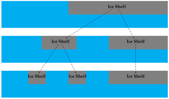
Figure 1.
Schematic showing the proposed sequential ice shelf breakup model. The upper panel shows the initial state in which there is a semi-infinite ice shelf. The middle and lower panels show the state after the first and second breakup events, respectively.
In this paper, we investigate the interaction between water waves and a row of multiple ice shelf fragments, or icebergs, positioned in front of a semi-infinite ice shelf. Our work extends the model of McNeil and Meylan [21], which studied the interaction of water waves with a single semi-infinite ice shelf (i.e., finite ice shelf fragments in front of the ice shelf were not considered). Following McNeil and Meylan, we cast the problem as a one-dimensional problem by invoking shallow water wave theory to model the hydrodynamics and Euler–Bernoulli beam theory to model the ice shelf vibrations. The resulting multiple scattering problem is solved using the transfer matrix method (TMM). In Section 2, we introduce the mathematical formulation of the problem and its solution in the frequency domain using the TMM. In Section 3, we use our frequency domain solutions to construct the solution in the time domain. Results are given in Section 4 to illustrate the capabilities of the model. In particular, we provide figures that describe wave energy reflection by the partially-fragmented ice shelf and show the temporal evolution of incident Gaussian wave packets. A brief conclusion is given in Section 5. Energy balance calculations, which are used to validate our results, are relegated to Appendix A.
2. Mathematical Model
2.1. Preliminaries
We consider the interaction of water waves with floating ice shelf fragments with rectangular cross sections in front of a semi-infinite floating ice shelf, also having a rectangular cross section. The assumptions of shallow water hydroelasticity [26] are used to simplify the theoretical framework. The geometry and motions are assumed to be transitionally invariant in one horizontal direction. In addition, the motion of the fluid and of the ice shelves is assumed to be independent of depth, so that the problem becomes one-dimensional. In order to do so, we have assumed that the motion of the fluid is governed by shallow water wave theory, that is, the fluid is assumed to be incompressible and inviscid and undergoing irrotational motion, and the depth of the fluid is assumed to be small compared with the radius of curvature of the free surface [27]. Moreover, the motion of the ice shelves is modelled using Euler–Bernoulli beam theory, which assumes that (i) the ice shelf is straight with a uniform cross section throughout its length, (ii) the deflections are minimal relative to the length of the ice shelf, (iii) the ice shelves are uniform and isotropic in composition, with the cross-sectional dimensions being significantly smaller than the ice shelves’ lengths, and (iv) the beam is subjected only to axial and transverse forces [28]. The infinite horizontal domain of our problem is spanned by the coordinate and divided into regions , in which the fluid is bounded above by an ice shelf, and , in which the fluid is bounded above by a free surface, such that . Our paper builds towards the case where is the union of disjoint intervals of finite length and one semi-infinite interval, that is, . The simpler cases of a single finite ice shelf fragment and a single semi-infinite ice shelf (where and , respectively) are considered first.
The motion of the ocean–ice shelf system is determined by the displacement and the velocity potential of the fluid . In particular, describes the vertical displacement of the free surface of the fluid for , and the vertical displacement of the ice for . As a consequence of shallow water wave theory and Euler–Bernoulli beam theory, and U satisfy the following coupled system of partial differential equations.
where is the ice shelves’ flexural rigidity, and are the density of water and ice, respectively, and h is the ice shelves’ thickness. Moreover, E is the Young’s modulus of the ice shelves, which we take to be 11 GPa, and the Poisson’s ratio, v, is taken to be 0.33. We assume that kg m−3 and kg m−3. The constant of gravitational acceleration is ms−2 and H represents the depth of the water and . Note that (1a) would be equivalent to (1d) if D and h were zero. The potential, , must also satisfy the continuity of potential conditions
and the continuity of flux conditions
where the free edge conditions
where , and and are the sets of left and right endpoints of the ice shelves, respectively. For example, if , then and . Note that (2b) and (2c) take different forms at the left and right endpoints of the ice shelves, whereas the other matching conditions do not.
Initially, we assume time-harmonic motions with angular frequency , so that and . Substituting these expressions into (1) gives
We use (3c) to eliminate u from (3), which gives rise to the following sixth-order equations for :
When solving the frequency domain problem, we impose radiation conditions at the far field, meaning that scattered waves must be outgoing. Equation (4) can be restated as
2.2. Solution for a Finite Ice Shelf Fragment
We begin by solving the problem of wave scattering by a finite ice shelf fragment, namely, the case where . The geometry of the problem is illustrated in Figure 2. The general solution to (5) in this case is
where the wave number k is the positive solution to the shallow water dispersion relation
and are the six roots of the ice-covered dispersion relation
The roots of (8) appear in positive and negative pairs. The purely imaginary root was chosen to have a positive imaginary component and was denoted as , while the roots with nonzero real parts were chosen to have negative real components and were denoted as and . Equation (6) has ten constants. We seek to construct the right-to-left transfer matrix, so we assume that and are known. So, we end up with eight unknowns, necessitating eight corresponding equations. These equations are derived as follows.
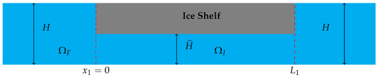
Figure 2.
Schematic of a finite ice shelf fragment.
When applied to the general solution (6), the continuity of the potential equation at (2a) implies that
Additionally, the flux continuity condition (2b) implies that
and the free edge conditions (2e) imply
Following the procedure outlined above at the right edge (i.e., at ), the matching conditions imply that
The conditions imposed by the matching conditions (9) give rise to a linear system of equations for the unknown coefficients of the form
where
The vector of unknown coefficients, X, can be obtained as
The transfer matrix for the ice shelf fragment describes the relationship between wave amplitudes to the left and right of the ice shelf fragment, respectively, and . To obtain this matrix, we momentarily discard information about the amplitudes of vibrations of the ice shelf itself, noting that they can be recovered from the water wave amplitudes using (10). To do so, we write
where
is the right-to-left transfer matrix and and are the identity matrix and zero matrix, respectively. We will make use of the transfer matrix described above when solving the multiple scattering problem for multiple fragments of the ice shelf in Section 2.4.
2.3. Solution for Semi-Infinite Ice Shelf
We introduce the solution for a semi-infinite ice shelf, which is the case . A schematic of the geometry of the problem is given in Figure 3. Assuming that there are no incoming waves propagating through the ice shelf from , the general solution is
Equation (14) has five constants, of which only is assumed to be known, and thus we require four corresponding equations. When applied to the general solution (14) at , the continuity of potential Equation (2a) implies that
Additionally, the continuity of flux condition (2b) implies that
The remaining two equations come from the free edge conditions (2d), which imply that
These conditions imposed by the matching conditions (15)–(18) give rise to a linear system of equations for the unknown coefficients of the form
where
The solution of the system above can be written as
The coefficients and are momentarily eliminated from the system by writing
where
We make use of this matrix when solving the multiple scattering problem. The remaining unknown coefficients, and , can subsequently be recovered from (19).
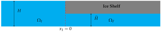
Figure 3.
Schematic of the problem for a semi-infinite ice shelf.
2.4. Multiple Scattering Solution
We apply the transfer matrix method to solve the multiple scattering problem of ice shelf fragments in front of a semi-infinite ice shelf, as illustrated in Figure 4. The transfer matrix method is briefly outlined here through the use of a diagram in Figure 5. Full details are given in [29,30]. The general solution to the multiple scattering problem is of the form
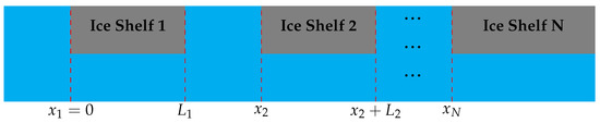
Figure 4.
Schematic of the problem of ice shelf fragments in front of a semi-infinite ice shelf.
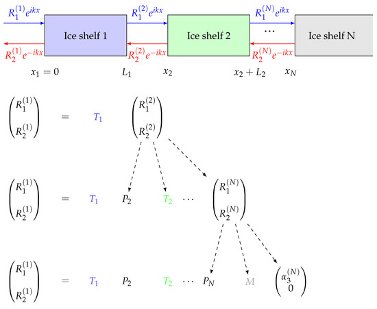
Figure 5.
Diagram outlining the transfer matrix method for the problem of ice shelf fragments in front of a semi-infinite ice shelf; the transfer matrix relates amplitudes to the left and right of the ice shelf. The amplitude to the right of ice shelf 1 is related to the amplitude to the left of ice shelf 2 via the propagating matrix, which is where . Repeating this process, we can obtain all the amplitudes in , and then we can recover the amplitudes under the ice. We seek to construct the right-to-left transfer matrix, so we assume that , and then we construct the transfer matrix for the whole array and we solve for , where . We can determine the amplitudes between the ice shelves using (12) for the ice shelf and (21) for the semi-infinite ice shelf. Once we have obtained those amplitudes, the remaining unknown coefficients can be recovered using (11) for the ice shelf and (20) for the semi-infinite ice shelf.
It is important to note that the transfer matrix method comprises two steps. The initial step involves employing the technique described in Figure 5 to determine . The subsequent step is to work backward to find all the remaining unknown coefficients. Note that the difference in the solution method between the two cases lies in the choice of roots. In the semi-infinite case, we select three specific roots and apply the boundary condition at the front, considering the ice shelf to be infinite. However, in the case of multiple scattering, we consider all six roots and apply boundary conditions at both the front and end of each ice shelf.
We present an overview of how we applied the transfer matrix method on multiple broken ice shelves that end with a semi-infinite ice shelf. In Section 2.2, we find the transfer matrix, T, for the finite ice shelf. This transfer matrix can be applied for multiple finite ice shelves by applying a new propagating matrix, which will be explained below. In Section 2.3, we provide the transfer matrix, M, for a semi-infinite ice shelf. Based on that, we are introducing the whole system as shown in Figure 5.
2.5. Energy Conservation
The conservation of energy relation for the system of ice shelf fragments in front of a semi-infinite ice shelf, which we used to validate our numerical calculations, is
which is identical to the relation derived in [21] for a single semi-infinite ice shelf. Our derivation of (24) is given in Appendix A. Note that similar results can be found in [31].
3. Time Domain Solution
We write the time dependent displacement, U, as a superposition of the frequency domain solutions as below
where . We calculate the integral numerically at the points using the midpoint rule
where are the quadrature weights. An application of this rule to (25) gives
Following observations outlined in [32,33], we can represent this sum as a matrix multiplication of the form
where the elements of are
and and have entries and , respectively. In this paper, we take the spectrum to describe an incident Gaussian wave packet
where the standard deviation, , describes the width of the Gaussian in the frequency domain and and is the peak frequency.
4. Results
We consider the case of two broken ice shelves, each of length 40 km, in front of a semi-infinite ice shelf. Both of the gaps between the ice shelves are of length 20 km. We evaluated the solution in the time domain using several values of ice shelf thickness, namely m, m, m, and m. We chose the parameters of the incident Gaussian wave packet to be m−1 and , and fixed the depth of the water to be m. Figure 6, Figure 7, Figure 8 and Figure 9 illustrate that, although there is not a significant change in wavelength as the wave packet enters the ice shelf, there can be a significant change in amplitude when the ice shelf is thick.
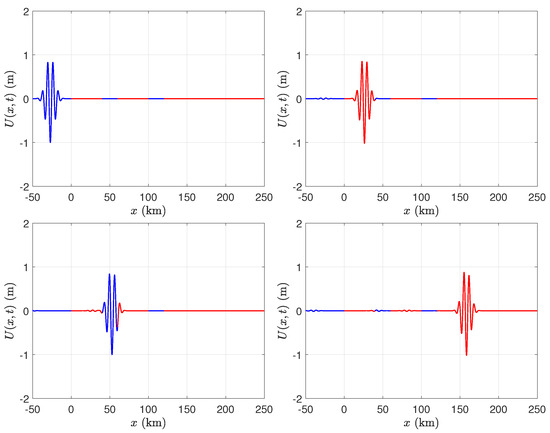
Figure 6.
Time-dependent displacement of the water wave–ice shelf system due to an incident Gaussian wave packet. The blue line segments indicate the displacement of the free surface of the water, while the red line segments indicate the vertical displacement of the ice, with a thickness of m and a same length of 40 km and 20 km water gaps, showing how the ice shelves respond to wave forces.
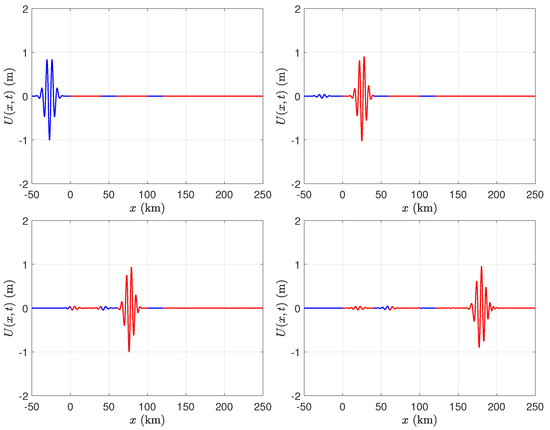
Figure 7.
As in Figure 6, with m.
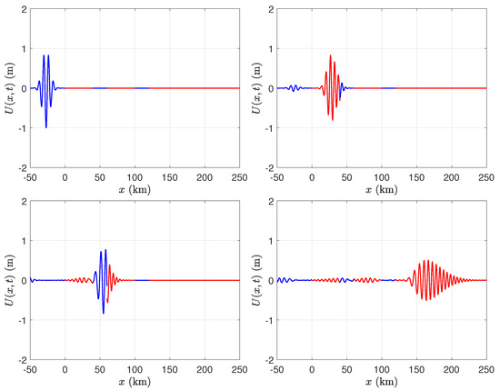
Figure 8.
As in Figure 6, with m.
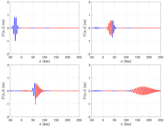
Figure 9.
As in Figure 6, with m.
Motivated by the conservation of energy identity (24), the reflected and transmitted energy by the ice shelves are defined to be
respectively. Figure 10 show the effect of frequency on the total transmitted and reflected energy.
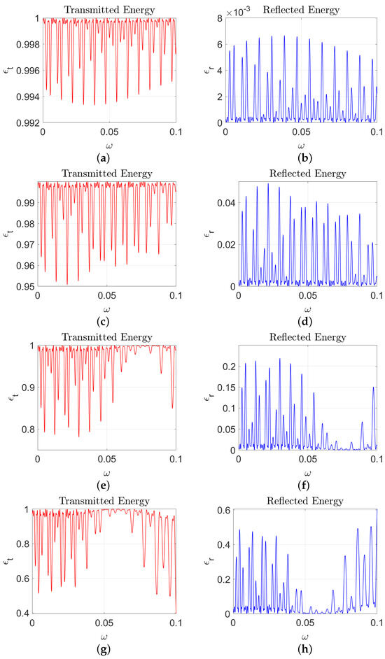
Figure 10.
The propagation of water waves over ice shelves of varying thicknesses. Panels (a,b) depict the transmitted and reflected energy for a thin ice shelf (), showing significant transmission of wave energy. Panels (c,d) illustrate a thicker ice shelf (), with a balance of transmitted and reflected energy. Panels (e,f) show a substantially thicker ice shelf (), resulting in reduced transmitted energy. Panels (g,h) depict the very thick ice shelf (), which strongly reflects wave energy, demonstrating significant wave attenuation.
Figure 11 show the effect of the Young’s modulus on the total reflected energy (similar figures would be found for transmitted). As expected, the reflected energy is lower for a lower Young’s modulus, although the effect is not very strong. We note that the Young’s modulus is not well parameterised for ice shelves.
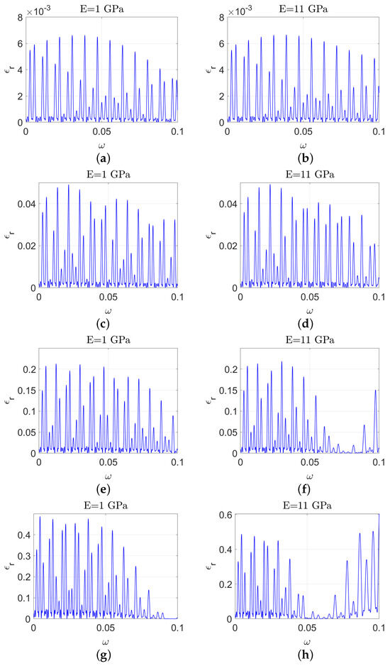
Figure 11.
The propagation of water waves over ice shelves of varying thicknesses is illustrated as follows. Panels (a,b) show the reflected energy for a thin ice shelf with a thickness of (). Panels (c,d) depict the reflected energy for a moderately thick ice shelf with a thickness of (). Panels (e,f) present the reflected energy for a significantly thicker ice shelf with a thickness of (). Panels (g,h) illustrate the reflected energy for a very thick ice shelf with a thickness of (). The figures on the left have a lower value for Young’s modulus compared to those on the right, as shown in the figure title.
There is a significant difference in the amount of reflected energy when there are a few ice shelf fragments in front of the semi-infinite ice shelf (see Figure 12). We hypothesise that this is due to resonant interactions caused by the gaps in the ice cover. In particular, the peaks in the reflection coefficients are reminiscent of stop bands, which is expected since the region containing ice shelf fragments is periodic.
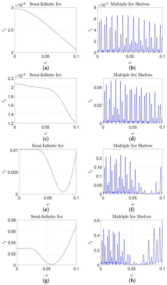
Figure 12.
The propagation of water waves over ice shelves of varying thicknesses is illustrated as follows. Panels (a,b) show the reflected energy for a thin ice shelf with a thickness of (). Panels (c,d) depict the reflected energy for a moderately thick ice shelf with a thickness of (). Panels (e,f) present the reflected energy for a significantly thicker ice shelf with a thickness of (). Panels (g,h) illustrate the reflected energy for a very thick ice shelf with a thickness of (). Panels (a,c,g) show the reflected energy for multiple ice shelves, while Panels (b,d,f) represent the reflected energy for semi-infinite ice shelves.
5. Conclusions
This study provides a simple model of water wave scattering by an array of floating ice shelf fragments in front of a semi-infinite ice shelf, which extends the previous work of [21]. By invoking the shallow water approximation and Euler–Bernoulli beam theory, we obtained a multiple scattering problem, which we solved using the transfer matrix method. Although we do not deny that these are significant assumptions, they were incredibly beneficial in giving rise to a tractable model that is computationally inexpensive to solve. Future work could seek to evaluate the effect of these assumptions in comparison with models with fewer assumptions or field data. Our work is an important step towards building a time domain model of sequential ice shelf disintegration.
Author Contributions
Conceptualization, M.H.M. and F.A.; methodology, M.H.M. and F.A.; software, F.A.; validation, F.A.; writing—original draft preparation, F.A.; writing—review and editing, M.H.M. and B.W.; visualization, F.A.; supervision, M.H.M. and B.W. All authors have read and agreed to the published version of the manuscript.
Funding
This research was funded partially by the Australian Government through the Australian Research Council, Discovery Grant, DP230100947.
Data Availability Statement
The raw data supporting the conclusions of this article will be made available by the authors on request.
Conflicts of Interest
The authors declare no conflicts of interest.
Appendix A. Energy Balance Calculation
From the following integral, we can calculate the conservation of energy, where L was chosen to be sufficiently large, i.e., and . Next, consider
and end up with
noting that the boundary terms that arise from integration by parts at cancel. Likewise,
Again, the boundary terms cancel. We observe that the terms for u at x = 0 cancel because of the edge conditions. When these expressions are combined, the result is:
Now, we substitute the terms for u and f and take the limit at L → ∞ (only needed for x > 0, where the evanescent roots are). With this limit, we have
Then, the energy balance relationship is
References
- Frederikse, T.; Landerer, F.; Caron, L.; Adhikari, S.; Parkes, D.; Humphrey, V.W.; Dangendorf, S.; Hogarth, P.; Zanna, L.; Cheng, L.; et al. The causes of sea-level rise since 1900. Nature 2020, 584, 393–397. [Google Scholar] [CrossRef]
- Thomas, R.H. Ice shelves: A review. J. Glaciol. 1979, 24, 273–286. [Google Scholar] [CrossRef]
- Scambos, T.; Bohlander, J.; Shuman, C.; Skvarca, P. Glacier acceleration and thinning after ice shelf collapse in the Larsen B embayment, Antarctica. Geophys. Res. Lett. 2004, 31, 3–7. [Google Scholar] [CrossRef]
- Holdsworth, G.; Glynn, J.E. Iceberg calving from floating glaciers by a vibrating mechanism. J. Geophys. Res. 1978, 274, 464–466. [Google Scholar] [CrossRef]
- Holdsworth, G.; Glynn, J.E. A Mechanismfor the Formation of Large Iceberg. J. Geophys. Res. 1981, 86, 3210–3222. [Google Scholar] [CrossRef]
- Brunt, K.M.; Okal, E.A.; Macayeal, D.R. Antarctic ice-shelf calving triggered by the Honshu (Japan) earthquake and tsunami, March 2011. J. Glaciol. 2011, 57, 785–788. [Google Scholar] [CrossRef]
- Cathles Iv, L.M.; Okal, E.A.; Macayeal, D.R. Seismic observations of sea swell on the floating Ross Ice Shelf, Antarctica. J. Geophys. Res. 2009, 114, 1–11. [Google Scholar] [CrossRef]
- Bromirski, P.D.; Sergienko, O.V.; MacAyeal, D.R. Transoceanic infragravity waves impacting antarctic ice shelves. Geophys. Res. Lett. 2010, 37, 1–6. [Google Scholar] [CrossRef]
- Brunt, K.M.; King, M.A.; Fricker, H.A.; Macayeal, D.R. Flow of the Ross ice Shelf, Antarctica, is modulated by the ocean tide. J. Glaciol. 2010, 56, 157–161. [Google Scholar] [CrossRef]
- MacAyeal, D.R.; Okal, E.A.; Aster, R.C.; Bassis, J.N.; Brunt, K.M.; Cathles, L.M.; Drucker, R.; Flicker, H.A.; Kim, Y.J.; Martin, S.; et al. Transoceanic wave propagation links iceberg calving margins of Antarctica with storms in tropics and Northern Hemisphere. Geophys. Res. Lett. 2006, 33, 1–4. [Google Scholar] [CrossRef]
- Bromirski, P.D.; Stephen, R.A. Response of the Ross Ice Shelf, Antarctica, to ocean gravity-wave forcing. Ann. Glaciol. 2012, 53, 163–172. [Google Scholar] [CrossRef]
- Bromirski, P.D.; Diez, A.; Gerstoft, P.; Stephen, R.A.; Bolmer, T.; Wiens, D.A.; Aster, R.C.; Nyblade, A. Ross ice shelf vibrations. Geophys. Res. Lett. 2015, 42, 7589–7597. [Google Scholar] [CrossRef]
- DeConto, R.M.; Pollard, D. Contribution of Antarctica to past and future sea-level rise. Nature 2016, 531, 591–597. [Google Scholar] [CrossRef] [PubMed]
- Massom, R.A.; Scambos, T.A.; Bennetts, L.G.; Reid, P.; Squire, V.A.; Stammerjohn, S.E. Antarctic ice shelf disintegration triggered by sea ice loss and ocean swell. Nature 2018, 558, 383–389. [Google Scholar] [CrossRef]
- Chen, Z.; Bromirski, P.D.; Gerstoft, P.; Stephen, R.A.; Wiens, D.A.; Aster, R.C.; Nyblade, A.A. Ocean-excited plate waves in the Ross and Pine Island Glacier ice shelves. J. Glaciol. 2018, 64, 730–744. [Google Scholar] [CrossRef]
- Chen, Z.; Bromirski, P.D.; Gerstoft, P.; Stephen, R.A.; Lee, W.S.; Yun, S.; Olinger, S.D.; Aster, R.C.; Wiens, D.A.; Nyblade, A.A. Ross Ice Shelf Icequakes Associated with Ocean Gravity Wave Activity. Geophys. Res. Lett. 2019, 46, 8893–8902. [Google Scholar] [CrossRef]
- Vaughan, D.G. Tidal flexure at ice shelf margins. J. Geophys. Res. 1995, 100, 6213–6224. [Google Scholar] [CrossRef]
- Schmeltz, M.; Rignot, E.; MacAyeal, D. Tidal flexure along ice-sheet margins: Comparison of InSAR with an elastic-plate model. Ann. Glaciol. 2002, 34, 202–208. [Google Scholar] [CrossRef]
- Sergienko, O.V. Normal modes of a coupled ice-shelf/sub-ice-shelf cavity system. J. Glaciol. 2013, 59, 76–80. [Google Scholar] [CrossRef]
- Bennetts, L.G.; Meylan, M.H. Complex resonant ice shelf vibrations. Soc. Ind. Appl. Math. 2021, 81, 1483–1502. [Google Scholar] [CrossRef]
- McNeil, S.; Meylan, M.H. Time-Dependent Modelling of the Wave-Induced Vibration of Ice Shelves. J. Mar. Sci. Eng. 2023, 11, 1191. [Google Scholar] [CrossRef]
- Aljabri, R.; Meylan, M.H. Time Domain Vibration Analysis of an Ice Shelf. J. Mar. Sci. Eng. 2024, 12, 468. [Google Scholar] [CrossRef]
- Kalyanaraman, B.; Bennetts, L.G.; Lamichhane, B.; Meylan, H. On the shallow-water limit for modelling ocean-wave induced ice-shelf vibrations. Wave Motion 2019, 90, 1–16. [Google Scholar] [CrossRef]
- England, M.R.; Wagner, T.J.W.; Eisenman, I. Modeling the breakup of tabular icebergs. Sci. Adv. 2020, 6, eabd1273. [Google Scholar] [CrossRef] [PubMed]
- Mokus, N.G.A.; Montiel, F. Wave-triggered breakup in the marginal ice zone generates lognormal floe size distributions: A simulation study. Cryosphere 2022, 16, 4447–4472. [Google Scholar] [CrossRef]
- Meylan, M.H. Spectral solution of time-dependent shallow water hydroelasticity. J. Fluid Mech. 2002, 454, 387–402. [Google Scholar] [CrossRef]
- Stoker, J.J. Water Waves: The Mathematical Theory with Applications; New York Interscience Publishers: New York, NY, UDA, 1957. [Google Scholar] [CrossRef]
- Chen, J. Nonlocal Euler—Bernoulli Beam Theories; Springer: Cham, Switzerland, 2021. [Google Scholar] [CrossRef]
- Bronson, R.; Costa, G.B. Matrix Methods: Applied Linear Algebra, 3rd ed.; Academic Press: Cambridge, MA, USA, 2009. [Google Scholar] [CrossRef]
- Martin, P.A. N masses on an infinite string and related one-dimensional scattering problems. Wave Motion 2014, 51, 296–307. [Google Scholar] [CrossRef]
- Papathanasiou, T.K.; Karperaki, A.E.; Belibassakis, K.A. On the resonant hydroelastic behaviour of ice shelves. Ocean Model. 2019, 133, 11–26. [Google Scholar] [CrossRef]
- Wilks, B.; Meylan, M.H.; Montiel, F.; Wakes, S. Generalised eigenfunction expansion and singularity expansion methods for canonical time-domain wave scattering problems. arXiv 2023. [Google Scholar] [CrossRef]
- Wilks, B.; Meylan, M.H.; Montiel, F.; Wakes, S. Generalised eigenfunction expansion and singularity expansion methods for two-dimensional acoustic time-domain wave scattering problems. arXiv 2023. [Google Scholar] [CrossRef]


Disclaimer/Publisher’s Note: The statements, opinions and data contained in all publications are solely those of the individual author(s) and contributor(s) and not of MDPI and/or the editor(s). MDPI and/or the editor(s) disclaim responsibility for any injury to people or property resulting from any ideas, methods, instructions or products referred to in the content. |
© 2024 by the authors. Licensee MDPI, Basel, Switzerland. This article is an open access article distributed under the terms and conditions of the Creative Commons Attribution (CC BY) license (https://creativecommons.org/licenses/by/4.0/).