Effective Quantum Graph Models of Some Nonequilateral Graphyne Materials

Abstract

It is shown that it is possible to adapt the quantum graph model of graphene to some types of nonequilateral graphynes considered in the literature; we also discuss the corresponding nanotubes. The proposed models are, in fact, effective models and are obtained through selected boundary conditions and an ad hoc prescription. We analytically recover some results from the literature, in particular, the presence of Dirac cones for $\alpha$-, $\beta$- and $(6,6,12)$-graphynes; for $\gamma$-graphyne, our model presents a band gap (according to the literature), but only for a range of parameters, with a transition at a certain point with quadratic touch and then the presence of Dirac cones.

1. Introduction

There are many proposals of two-dimensional carbon allotropes in the literature, with graphene being the most prominent due to its peculiar electronic properties, and it has been synthesized since 2004 (see the review [1]). Theoretical techniques to study graphene, both single and multilayer cases, include ab initio calculations (comprising the density functional theory) and tight-binding models. On the rigorous mathematical side, there are three approaches for single layer graphene in the literature: one continuous model by Fefferman and Weinstein [2] proving the “generic” presence of Dirac cones in the dispersion relations; interesting symmetry arguments by Berkolaiko and Comech [3], and this method applies to different settings, including some multilayer models; and a quantum graph model (QGM), mainly due to Amovilli, Leys and March [4] and Kuchment and Post [5]. The latter approach has two advantages: it is simpler then the previous one and permits an accurate spectral analysis including details of Dirac cones; however, this technique requires that all edges in the graph have the same length, that is, an equilateral graph. Recently, the present authors have proposed adaptations in the boundary conditions so that the AA- and AB-stacked graphene multilayer could (at least qualitatively) be modeled by QGMs [6,7]; there is a work that also covers a few layers of graphene combined with hexagonal boron nitride [8] (again with a QGM).

In this work, we discuss how to (approximately) describe some distinct structures of graphynes via QGMs, including cases with edges of different lengths, again by playing with boundary conditions, and our main interest is in the possible presence of Dirac cones; ad hoc assumptions will be employed, and our results are compatible with some known results in the literature. We also discuss graphyne nanotubes in this context. Although our approach may seem rather exploratory, the results are mathematically correct, and it was not without some surprise that such proposal has worked!

The structure of graphynes are obtained from that of graphene. Recall that all carbon atoms in the graphene equilateral hexagonal lattice (we reserve the term honeycomb to such a regular hexagonal lattice) have ${\mathrm{sp}}^2$ hybridization with single and double bonds. Carbon atoms in graphynes have both ${\mathrm{sp}}^2$ and $\mathrm{sp}$ hybridizations, and they are usually obtained by replacing selected single $\mathrm{C}\left({\mathrm{sp}}^2\right)-\mathrm{C}\left({\mathrm{sp}}^2\right)$ bonds in graphene with

$$\mathrm{C}\left({\mathrm{sp}}^2\right)-\mathrm{C}\left(\mathrm{sp}\right)\equiv \mathrm{C}\left(\mathrm{sp}\right)-\mathrm{C}\left({\mathrm{sp}}^2\right)$$

ones [9], which then also include triple bonds. Graphynes were predicted by Baughman, Eckhardt and Kertesz [10] in 1987 and only small samples have been synthesized; however, recently [11,12], a scalable synthesis was obtained, and some authors advocate that graphyne might replace graphene [13].

Some graphynes are expected to present Dirac cones, which were theoretically found in first-principle calculations [14], tight-binding models [9] and, in a particular case for which all edges have the same length [15], through a QGM (and Dirac cones were found). Perhaps this work could be seen as a step forward for some parts of [15].

Here, we extend the QGM to four types of graphynes considered in [9,14] (see also [16]); they are shown in Figure 1 and named $\alpha$-, $\beta$-, $\gamma$- and (6,6,12)-graphynes. In short, we always think of the graphene honeycomb lattice, and for each edge, we introduce a positive parameter in the boundary conditions (see (4)) at vertices, in order to take into account the intensity of the chemical bond in each edge; the stronger the bond, the larger the parameter value. This will permit us to model some graphynes whose edges have different lengths, i.e., nonequilateral ones, in terms of the honeycomb structure; it should be clear that we have just effective models, which include some heuristic arguments, since the honeycomb structure of such models may differ from the graphyne structures (and this is a strength of our approach).

After modeling with QGMs, in many instances, the calculations are rigorous and analytical, so they are without approximations (sometimes we appeal to the plots of the graphs of functions to guide us about the possible existence of zeros). We summarize our findings as follows:

• $\alpha$-graphyne has the peculiarity of edges with three double bonds, and others with two single and a triple bonds. We argue (see ahead) that, from the point of view of QGMs, they have comparable bond strengths, so our model reproduces the one of graphene [5] in this case. Hence, we do not explore $\alpha$-graphene in this work (we just include some remarks for completeness with respect to [9,14]).
• In accordance with other works [9,14], we have obtained that Dirac points are present in $\beta$-graphyne.
• In the literature [9], a band gap was found (with no Dirac cone, of course) for the $\gamma$-graphyne. Our QGM shows a richer structure in this case; there is a transition at a certain parameter value $t=t_c$ (see ahead for details), with a gap band between valence and conduction bands for $0<t<t_c$, Dirac cones for $t_c<t<1$ and at the transition point $t=t_c$, there is a parabolic touch. We have an explicit description of the gap size as a function of the parameters. Such properties should be of interest to be confirmed by experimentalists, in particular because it opens a potential for practical applications of $\gamma$-graphyne.
  It is worth mentioning that this is one of the graphynes in which a scalable synthesis has been recently obtained [11].
• Our effective QGM of (6,6,12)-graphyne also presents Dirac cones for all values of the parameters, with two different Dirac points, in agreement with [9,14]. This case is technically more involved than the others, so that we have checked that there are no other touch points by looking at the graph of the dispersion relations (instead of just analytical expressions as in the other cases). We have not found that it is “self-doped” as reported in [14] (note that this property was not reported in a tight-binding calculation [9] either).
• For the graphynes we consider, we discuss conditions so that the Dirac cones stay present after building graphyne tubes.
• In all cases with Dirac cones, they are explicitly located and the cone slopes are given in terms of the parameters of the model.

In Section 2, the general idea of the QGM is presented in the specific case of the honeycomb lattice (since we propose to (effectively) think of all considered cases with the structure of this lattice), with some heuristics and the proposed choices of boundary conditions. In Section 3, a general discussion about dispersion relations of such QGMs is performed, which is then, in Section 4, specialized to Dirac cones in each considered graphyne type. Nanotubes are the subject of Section 5. Conclusions appear in Section 6.

2. Honeycomb Quantum Graph Model

2.1. Graphene Graph Model: A Short Account

Now, we briefly discuss the graphene quantum graph employed by Amoville, Leys and March [4] and mainly by Kuchment and Post [5] (see these works for precise details). Let G be the honeycomb lattice, the hexagonal 2D structure shown in Figure 2a (see Section 2.1.1), and let the Hilbert space ${\mathrm{L}}^2\left(G\right):={⨁}_e{\mathrm{L}}^2\left(e\right)$ consist of all the square integrable functions on G. The free (i.e., no potential) graphene Hamiltonian H acting in functions $u\in {\mathrm{L}}^2\left(G\right)$ along each edge e is given by

$$H{u}_e\left(x\right)=-\frac{{\mathrm{d}}^2{u}_e}{\mathrm{d}{x}^2}\left(x\right),$$

(1)

satisfying the so-called Neumann vertex conditions at the vertices. These conditions requires the continuity of the functions and vanishing of the total flux at each vertex v, that is, $u_{e_1}\left(v\right)=u_{e_2}\left(v\right)=u_{e_3}\left(v\right)$ and $u_{e_1}^{\prime }\left(v\right)+u_{e_2}^{\prime }\left(v\right)+u_{e_3}^{\prime }\left(v\right)=0$, respectively.

From the Floquet–Bloch theory, the study of the Hamiltonian H is reduced to the study of the family of Bloch Hamiltonians $H\left(\theta \right)$, where $\theta =({\theta }_1,{\theta }_2)$ is the quasimomentum in the Brillouin zone $B:={[-\pi ,\pi ]}^2$. These operators $H\left(\theta \right)$ act the same way H does, but in functions that satisfy, in addition to the Neumann vertex conditions, the Floquet condition (see (6)). Moreover, $H\left(\theta \right)$ has a purely discrete spectrum and the graph of the function $\theta \mapsto \sigma \left(H\right(\theta \left)\right)$ is the dispersion relation of H. The range of this function is the spectrum of H, that is, $\sigma \left(H\right)$ is given by the reunion of $\sigma \left(H\right(\theta \left)\right)$, $\theta \in B$.

Thus, in order to determine the spectrum of H and its dispersion relation, we have to solve the eigenvalue problem

$$H\left(\theta \right)u=\lambda u,\lambda \in \mathbb{R},$$

which is done by employing two auxiliary operators, that is, one of them with the action (1) and Dirichlet boundary condition, and the other a periodic (one-dimensional) Hill operator.

After calculations, one obtains an explicit dispersion relation depending on the function (compare with (15))

$$\begin{array}{ccc}\hfill g\left(\theta \right)& =& {\displaystyle \sqrt{(1+e^{i{\theta }_1}+e^{i{\theta }_2})(1+e^{-i{\theta }_1}+e^{-i{\theta }_2})}}\hfill \\ \hfill & =& {\displaystyle \sqrt{1+8cos\frac{{\theta }_1-{\theta }_2}{2}cos\frac{{\theta }_1}{2}cos\frac{{\theta }_2}{2}}.}\hfill \end{array}$$

In particular, it can be shown that the dispersion relation has Dirac cones at the points $\pm (2\pi /3,-2\pi /3)$ of the Brillouin zone.

In the following, particularly in Section 3 and Section 4, we shall present details of this method adapted and applied to some graphynes.

2.1.1. Graphyne Sheet Model

The honeycomb lattice G is generated by the union of two triangular sublattices, $g_A$ (with vertices of type A) and $g_B$ (with vertices of type B), where

$$g_A:=\mathbb{Z}{E}_1+\mathbb{Z}{E}_2\mathrm{and}{g}_B:=g_A+(1,0),$$

with $E_1=(3/2,\sqrt{3}/2)$ and $E_2=(0,\sqrt{3})$ being the lattice vectors (see Figure 2a). Consider the action of the group ${\mathbb{Z}}^2$ on G using shift by the vectors $p_1{E}_1+p_2{E}_2$, $p=(p_1,p_2)\in {\mathbb{Z}}^2$, with a fundamental domain (or Wigner–Seitz cell) $W=\{v_1,v_2,a_1,a_2,a_3\}$ (see Figure 2b).

We identify each edge e of G with the segment $[0,1]$, denote by $E\left(G\right)$ the set of edges of G and by $E_v\left(G\right)$, the set of three edges that contains the vertex v.

The proposed Hamiltonian operator H acts along each edge $e\in E\left(G\right)$ as the free operator (see Remark 4) in suitable units,

$$H{u}_e\left(x\right)=-\frac{{\mathrm{d}}^2{u}_e}{\mathrm{d}{x}^2}\left(x\right),x\in e,$$

(2)

satisfying the modified Neumann vertex conditions in each vertex v of G; let $E_v\left(G\right)=\{e_1,e_2,e_3\}$:

(i)

Modified continuity condition:

$$\frac{u_{e_1}\left(v\right)}{t_1}=\frac{u_{e_2}\left(v\right)}{t_2}=\frac{u_{e_3}\left(v\right)}{t_3}.$$

(3)

(ii)

Modified zero total flux condition:

$$t_1{u}_{e_1}^{\prime }\left(v\right)+t_2{u}_{e_2}^{\prime }\left(v\right)+t_3{u}_{e_3}^{\prime }\left(v\right)=0.$$

(4)

The derivatives $u_{e_j}^{\prime }\left(v\right)$ are directed from v to the other vertex of $e_j$ and $t_1$, $t_2$ and $t_3$ are the positive interaction parameters between the edge bonds. Our idea is that the larger the bond strength in an edge (so the larger the parameter value), the larger its contribution to the flux at each vertex and the larger the value of the function at the vertex (due to the division by the parameter). The values of such parameters depend on each considered graphyne.

We call the general operator H a graphyne operator. Under these conditions, the graphyne operator is self-adjoint, as discussed in Appendix A.

Remark 1. 

From (4), one may suppose that the maximum value among the parameters $t_1,t_2,t_3$ takes the value 1. For instance, in case $t_1$ takes the maximum value, one may write (4) in the form

$$t_1\left(u_{e_1}^{\prime }\left(v\right)+{\tilde{t}}_2{u}_{e_2}^{\prime }\left(v\right)+{\tilde{t}}_3{u}_{e_3}^{\prime }\left(v\right)\right)=0,$$

with $0<{\tilde{t}}_2=t_2/t_1\le 1$ and $0<{\tilde{t}}_3=t_3/t_1\le 1$.

Remark 2. 

Note that graphene, as studied in [5], is recovered by selecting $t_1=t_2=t_3$. This simple remark has an important consequence for this work: it tells us that in the QGM of graphene, the single and double bonds have effectively the same intensity, and we will assume this while modeling graphynes. We have checked, in some cases, that our results are essentially the same whether we slightly distinguish the intensities of single and double bonds (not shown here), but we pay the price of much more complicated expressions to deal with.

By taking into account the above remarks, let us describe some heuristics and the proposed parameter ranges in each graphyne case shown in Figure 1.

(i)

The lattice is always the honeycomb one, i.e., the equilateral hexagonal lattice in Figure 2a; we technically require that all edges have the same length (e.g., due to the representation (18));

(ii)

For each graphyne, we look at its structure (Figure 1) and select edges that will be associated with $a_1,a_2,a_3$ in the fundamental domain W of the honeycomb lattice (Figure 2b), thus identifying the values of parameters $t_1,t_2,t_3$ (recall that the larger the bond strength, the larger the corresponding parameter; note that $a_1$ differs from the other edges since it is the unique that connects the two vertices in W).

(iii)

By looking at Figure 1, we identify four types of edge bonds $b_1,\cdots ,b_4$, whose bond strengths will be probed (and compared) by their well-known enthalpy values (http://www.wiredchemist.com/chemistry/data/bond_energies_lengths.html, accessed on 23 May 2023):

• $b_1$ representing $\mathrm{C}-\mathrm{C}$ and known enthalpy $h_1=346$ kJ/mol;
• $b_2$ representing $\mathrm{C}=\mathrm{C}$ and enthalpy $h_2=602$ kJ/mol;
• $b_3$ representing $\mathrm{C}=\mathrm{C}=\mathrm{C}=\mathrm{C}$ and enthalpy $h_3=1806$ kJ/mol (this bond only occurs in $\alpha$-graphyne);
• $b_4$ representing $\mathrm{C}-\mathrm{C}\equiv \mathrm{C}-\mathrm{C}$ and enthalpy $h_4=1527$ kJ/mol (this bond is part of all graphyne compositions).

In graphene, there occurs only $b_1$ and $b_2$ bonds, and they are considered indistinguishable from the point of view of QGMs [5]; their enthalpy difference is $h_2-h_1=256$ kJ/mol. Hence, bonds with an enthalpy difference of this order will not be distinguished in our modeling, and this is the case of $b_3$ and $b_4$, whose enthalpy difference is 279 kJ/mol (and $(h_3-h_4)/(h_2-h_1)\approx 1.09$). The other enthalpy values differ from at least 925 kJ/mol (the difference between $b_2$ and $b_4$ with $(h_4-h_2)/(h_2-h_1)\approx 3.6$), and so they will be considered distinct in the modeling.

(iv)

We need a criterion to associate two vertices and three graphyne edges in its fundamental domain (Figure 1) with those in W that could depict the main graphyne characteristics. It is natural to pick the most common configuration that appears in the fundamental cell of each graphyne; for $\beta$- and $\gamma$-graphynes, this procedure works, but not for the $(6,6,12)$-graphyne. So, for the latter case, we have worked with the options (that includes the bond $b_4$) and selected the one that has recovered results in [9,14].

Let’s apply the above procedure to the graphynes in Figure 1; see selections that are labeled $a_1,a_2,a_3$ in that figure:

• $\alpha$-graphyne: as anticipated, all edge bonds are supposed to be indistinguishable from the QGM viewpoint, so $t_1=t_2=t_3=1$; it then coincides with the graphene QGM (which is consistent to known results).
• $\beta$-graphyne: we have $t_2=t_3=1$ (since $a_2,a_3$ have $b_4$ bonds) and $0<t_1<1$ (because $a_1$ has a $b_2$ bond).
• $\gamma$-graphyne: we have $t_1=1$ and $0<t_2=t_3<1$.
• $(6,6,12)$-graphyne: we take $t_1=t_2=1$ and $0<t_3<1$.

Note that the choice associated with the $a_1$ edge, in all cases, point to a corner of the fundamental domain (there are two possibilities for the $(6,6,12)$ case), but we do not have any justification to take this as a criterion to select graphyne edges to be mapped to the honeycomb fundamental domain.

Remark 3. 

With the benzene ring being a resonant structure, its bonds, represented by successive alternating single and double bonds, are rigorously equivalent. Therefore, considering them equivalent has both experimental and theoretical foundations from a quantum mechanical point of view. This way, graphynes can be reduced to two different parameters: one associated with the benzene ring and the other with the acetylene group $\mathrm{C}-\mathrm{C}\equiv \mathrm{C}-\mathrm{C}$. However, the use of enthalpy values give quantitative relations with a potential to be applied to other situations.

Remark 4. 

As done in previous works [5,6,7,15], similar qualitative results are obtained by adding an even potential to the operator (2). We have opted to keep things simpler by selecting a free operator in each edge; furthermore, this choice gives explicit expressions for some spectral quantities.

2.1.2. Graphyne Nanotube Model

A carbon nanotube is a tube made of carbon with a diameter in nanoscale. There are many types of these materials (see [17] for a more detailed discussion of nanotubes), but here, we will keep our attention to the single-walled carbon nanotubes (SWCNTs) that can be obtained by cutouts of a two-dimensional hexagonal lattice. Depending on the cutout, we have different classifications of the SWCNTs. For instance, Figure 3a shows the so-called zig-zag nanotube, since it has a zig-zag closed path around the tube. Figure 3b shows the armchair nanotube, which is encircled by a closed path in the form of an armchair. Other types of nanotubes considered here are the chiral nanotubes.

Here, we discuss the propose of the corresponding single-wall graphyne nanotube models. A more detailed discussion and classification of graphene nanotubes can be find in [17] and the references therein.

Let $p\in {\mathbb{R}}^2\setminus \left\{0\right\}$ be a vector of the lattice of translation symmetries of the quantum graph G, that is, we can write p as

$$p=p_1{E}_1+p_2{E}_2,p_1,p_2\in \mathbb{Z}.$$

(5)

Let ${\sim }_p$ be the equivalence relation given by $z_1{\sim }_p{z}_2$ if, and only if, $z_2-z_1=q.p$, with $z_1,z_2\in G$ and q as an integer number. The graph $G_p$ obtained as the quotient of G with respect to the equivalence relation ${\sim }_p$ is proposed to model a graphyne nanotube. This graph is naturally isometrically embedded into the cylinder ${\mathbb{R}}^2/{\sim }_p$. If $p=(p_1,p_2)$, we denote $G_p=G_{(p_1,p_2)}$. There are several types of nanotubes. For instance, $G_{(N,0)}$ and $G_{(0,N)}$ are the so-called zig-zag nanotubes, $G_{(N,N)}$ are the armchair nanotubes and the chiral are nanotubes with the form $G_{(p_1,p_2)}$, with $p_1\ne p_2$, $p_1,p_2\ne 0$.

The corresponding Hamiltonian operator will be denoted by $H_p$, called the graphyne nanotube operator, which is defined exactly as the graphyne operator H above, with modified Neumann vertex conditions (2), and taking into account the above additional symmetry (see Section 5).

3. Dispersion Relation

Now, we derive the dispersion relation of the graphyne operator H; it is based on the Floquet–Bloch theory [18,19,20,21] combined with the idea [5] of considering spectral points outside the spectrum of the edge Dirichlet operator. We begin with the general model; then, we specialize to each graphyne case.

For each quasimomentum $\theta =({\theta }_1,{\theta }_2)$ in the Brillouin zone B, let $H\left(\theta \right)$ be the Bloch Hamiltonian acting on functions satisfying the conditions (3) and (4) and also the Floquet condition

$$u(x+p_1{E}_1+p_2{E}_2)=e^{i(p_1{\theta }_1+p_2{\theta }_2)}u\left(x\right),$$

(6)

for any $p=(p_1,p_2)\in {\mathbb{Z}}^2$ and $x\in W$. The spectra of $H\left(\theta \right)$ is constituted only of eigenvalues and denoted by $\sigma \left(H\left(\theta \right)\right)={\left\{{\lambda }_n\left(\theta \right)\right\}}_n$, and the spectrum of H is the union of these spectra (see [18]):

$$\sigma \left(H\right)=\bigcup _{\theta \in B}\sigma \left(H\left(\theta \right)\right).$$

(7)

Recall that the function $\theta \mapsto {\left\{{\lambda }_n\left(\theta \right)\right\}}_n$ is the dispersion relation of H. Thus, to determine $\sigma \left(H\right)$ and the dispersion relation of H, we have to solve the following eigenvalue problem for each quasimomentum $\theta \in B$:

$$H\left(\theta \right)u=\lambda u,\lambda \in \mathbb{R}.$$

(8)

In order to solve (8), consider the auxiliary operator $H^{\mathrm{D}}$, with action

$$H^{\mathrm{D}}u\left(x\right)=-\frac{{\mathrm{d}}^{2}u}{\mathrm{d}{x}^2}\left(x\right)$$

(9)

and the Dirichlet boundary condition, that is, $u\left(0\right)=u\left(1\right)=0.$ It is well known that $H^{\mathrm{D}}$ has the purely discrete spectrum $\sigma \left(H^{\mathrm{D}}\right)={\left\{k^2{\pi }^2\right\}}_{k\ge 1}$. If $\lambda \notin \sigma \left(H^{\mathrm{D}}\right)$, then there exist two linearly independent solutions, ${\phi }_{\lambda ,0}$ and ${\phi }_{\lambda ,1}$, of the eigenvalue problem

$$-{\phi }^{\prime \prime }=\lambda \phi ,\lambda \in \mathbb{R},$$

(10)

such that

$${\phi }_{\lambda ,0}\left(0\right)={\phi }_{\lambda ,1}\left(1\right)=1,$$

(11)

$${\phi }_{\lambda ,0}\left(1\right)={\phi }_{\lambda ,1}\left(0\right)=0,$$

(12)

$${\phi }_{\lambda ,1}^{\prime }\left(x\right)=-{\phi }_{\lambda ,0}^{\prime }(1-x),x\in [0,1].$$

(13)

Explicitly,

$${\phi }_{\lambda ,0}\left(x\right)=\frac{sin\left(\sqrt{\lambda }(1-x)\right)}{sin\sqrt{\lambda }},{\phi }_{\lambda ,1}\left(x\right)=\frac{sin\left(\sqrt{\lambda }x\right)}{sin\sqrt{\lambda }}.$$

The quotient

$$\eta \left(\lambda \right):=\frac{{\phi }_{\lambda ,1}^{\prime }\left(1\right)}{{\phi }_{\lambda ,1}^{\prime }\left(0\right)}=cos\sqrt{\lambda }$$

(14)

is well defined for $\lambda \notin \sigma \left(H^D\right)$.

Let $\lambda \notin \sigma \left(H^{\mathrm{D}}\right)$ and $0<t_j\le 1$, with $j=1,2,3$. Then, we claim that the real number $\lambda$ belongs to the spectrum of H if, and only if, there exists a quasimomentum $\theta \in B$ such that

$$\eta \left(\lambda \right)=\pm \frac{\sqrt{f\left(\theta \right)}}{T},$$

with $T=t_1^2+t_2^2+t_3^2$ and

$$f\left(\theta \right)=t_1^4+t_2^4+t_3^4+2t_1^2{t}_2^{2}cos\left({\theta }_1\right)+2t_1^2{t}_3^{2}cos\left({\theta }_2\right)+2t_2^2{t}_3^{2}cos({\theta }_1-{\theta }_2).$$

(15)

In order to conclude this, first, note that by the Floquet condition (6), we have (see Figure 2b)

$$u_{a_1}\left(v_2\right)=e^{i{\theta }_2}{u}_{a_2}\left(v_3\right)=e^{i{\theta }_2}{u}_{a_3}\left(v_4\right).$$

(16)

Thus, combining (16) with the modified Neumann vertex conditions, we obtain

$$\left\{\begin{array}{c}{u}_{a_1}\left(0\right)/t_1=u_{a_2}\left(0\right)/t_2=u_{a_3}\left(0\right)/t_3:=A\hfill \\ u_{a_1}\left(1\right)/t_1=e^{i{\theta }_1}{u}_{a_2}\left(1\right)/t_2=e^{i{\theta }_2}{u}_{a_3}\left(1\right)/t_3:=B\hfill \\ t_1{u}_{a_1}^{\prime }\left(0\right)+t_2{u}_{a_2}^{\prime }\left(0\right)+t_3{u}_{a_3}^{\prime }\left(0\right)=0\hfill \\ t_1{u}_{a_1}^{\prime }\left(1\right)+t_2{e}^{i{\theta }_1}{u}_{a_2}^{\prime }\left(1\right)+t_3{e}^{i{\theta }_2}{u}_{a_3}^{\prime }\left(1\right)=0\hfill \end{array}\right..$$

(17)

Thus, for u to be an eigenfunction of $H\left(\theta \right)$, it must satisfy (17).

Let $\lambda \notin \sigma \left(H^{\mathrm{D}}\right)$ and consider ${\phi }_{\lambda ,0}$ and ${\phi }_{\lambda ,1}$ as the linearly independent solutions of (10) that satisfy (11)–(13). We can represent $u_{a_j}$ as

$$\left\{\begin{array}{c}{u}_{a_1}=t_1(A{\phi }_{\lambda ,0}+B{\phi }_{\lambda ,1})\hfill \\ u_{a_2}=t_2(A{\phi }_{\lambda ,0}+e^{-i{\theta }_1}B{\phi }_{\lambda ,1})\hfill \\ u_{a_3}=t_3(A{\phi }_{\lambda ,0}+e^{-i{\theta }_2}B{\phi }_{\lambda ,1})\hfill \end{array}\right..$$

(18)

It is easy to see that the function defined by (18) satisfies the modified continuity condition (3) of the modified Neumann vertex condition and solves the eigenvalue problem (10). It remains to be verified that (18) satisfies the zero total flux condition (4). Substituting (18) into the last two equations of (17), we obtain

$$\left\{\begin{array}{c}(t_1^2+t_2^2+t_3^2){\phi }_{\lambda ,0}^{\prime }\left(0\right)A+(t_1^2+t_2^2{e}^{-i{\theta }_1}+t_3^2{e}^{-i{\theta }_2}){\phi }_{\lambda ,1}^{\prime }\left(0\right)B=0\hfill \\ (t_1^2+t_2^2{e}^{i{\theta }_1}+t_3^2{e}^{i{\theta }_2}){\phi }_{\lambda ,0}^{\prime }\left(1\right)A+(t_1^2+t_2^2+t_3^2){\phi }_{\lambda ,1}^{\prime }\left(1\right)B=0\hfill \end{array}\right..$$

(19)

With (13), ${\phi }_{\lambda ,0}^{\prime }\left(0\right)=-{\phi }_{\lambda ,1}^{\prime }\left(1\right)$ and ${\phi }_{\lambda ,0}^{\prime }\left(1\right)=-{\phi }_{\lambda ,1}^{\prime }\left(0\right)$. Substituting this into (19), then dividing by ${\phi }_1^{\prime }\left(0\right)\ne 0$ and multiplying by $-1$ its second equation, we obtain

$$\left\{\begin{array}{c}-T\eta \left(\lambda \right)A+\overline{F}\left(\theta \right)B=0\hfill \\ F\left(\theta \right)A-T\eta \left(\lambda \right)B=0\hfill \end{array}\right.,$$

(20)

with $F\left(\theta \right)=t_1^2+t_2^2{e}^{i{\theta }_1}+t_3^2{e}^{i{\theta }_2}$, $\overline{F}$ the complex conjugate of F and $T=t_1^2+t_2^2+t_3^2$. The determinant $\delta$ of this system equals

$$\delta =T^2\eta {\left(\lambda \right)}^2-f\left(\theta \right),$$

(21)

with $f\left(\theta \right)=F\left(\theta \right)\overline{F}\left(\theta \right)$, which is exactly (15). Hence, if there exists a quasimomentum $\theta \in B$ such that $\eta \left(\lambda \right)$ is one solution of $\delta =0$, that is,

$$\eta \left(\lambda \right)=\pm \frac{\sqrt{f\left(\theta \right)}}{T},$$

(22)

it follows that the representation (18) solves the eigenvalue problem (8) and so $\lambda \in \sigma \left(H\right)$ by (7). Therefore, the above claim is justified.

By (14), except possibly for $\lambda \in \sigma \left(H^{\mathrm{D}}\right)$, a discrete sequence of numbers, the dispersion relation of H is given by

$$cos\left(\sqrt{\lambda }\right)=\pm \frac{\sqrt{f\left(\theta \right)}}{T},\theta \in B,$$

(23)

with $f\left(\theta \right)$ given by (15). This description of the dispersion relation (23) of the graphyne operator H will allow us to study the possible presence of Dirac cones. In the next section, we present such an analysis.

4. Dirac Cones

We make use of (23) to study the possible presence of Dirac cones. We specialize in each case: $\beta$-graphyne, $\gamma$-graphyne and $(6,6,12)$-graphyne. Recall that a Dirac cone is a point where, in the lowest order approximation, the valence and conduction bands linearly touch each other, and the quasimomentum ${\theta }_D\in B$ for which a Dirac cone occurs is called a D-point. In symbols, if ${\theta }_D\in B$ is a D-point, then there is a constant $\gamma \ne 0$ so that

$$\lambda \left(\theta \right)-\lambda \left({\theta }_D\right)=\pm \gamma |\theta -{\theta }_D|+\mathcal{O}(|\theta -{\theta }_D{|}^2)+\mathcal{O}({\left(\lambda \left(\theta \right)-\lambda \left({\theta }_D\right)\right)}^2),$$

(24)

with the “−” and “+” signs for the valence and conduction bands, respectively.

Let $\lambda \notin \sigma \left(H^D\right)$. By (23), if ${\eta }_{\pm }(\lambda ,\theta )$ are the two roots of (21), given by

$${\eta }_{\pm }(\lambda ,\theta )=\pm \frac{\sqrt{f\left(\theta \right)}}{t_1^2+t_2^2+t_3^2},$$

(25)

in order to obtain Dirac cones, one must find D-point candidates ${\theta }_D\in B$ and expand $D\left(\lambda \right)=cos\left(\sqrt{\lambda }\right)$ and ${\eta }_{\pm }(\lambda ,\theta )$ around $\lambda \left({\theta }_D\right)$ and ${\theta }_D$, respectively. Then, if ${\theta }_D$ is a D-point, expanding $D\left(\lambda \right)$ around $\lambda \left({\theta }_D\right)$,

$$D\left(\lambda \left(\theta \right)\right))=D\left(\lambda \left({\theta }_D\right)\right)+D^{\prime }\left(\lambda \left({\theta }_D\right)\right)(\lambda \left(\theta \right)-\lambda \left({\theta }_D\right))+\mathcal{O}\left({(\lambda \left(\theta \right)-\lambda \left({\theta }_D\right))}^2\right),$$

(26)

which implies

$$D\left(\lambda \left(\theta \right)\right)-D\left(\lambda \left({\theta }_D\right)\right)=c\left({\theta }_D\right)(\lambda \left(\theta \right)-\lambda \left({\theta }_D\right))+\mathcal{O}\left({(\lambda \left(\theta \right)-\lambda \left({\theta }_D\right))}^2\right),$$

(27)

with $c\left({\theta }_D\right)=\left({\lambda }^{\prime }\left({\theta }_D\right)sin\sqrt{\lambda \left({\theta }_D\right)}\right)/\sqrt{\lambda \left({\theta }_D\right)}$; finally,

$$\lambda \left(\theta \right)={\left(arccos\left({\eta }_{\pm }(\lambda ,\theta )\right)+k\pi \right)}^2,k\in \mathbb{Z}.$$

(28)

Hence, if ${\theta }_D$ is a D-point candidate, we have the explicit parameter $c\left({\theta }_D\right)$. Therefore, it remains to be analyzed, in each type of graphyne, the possible presence of D-points.

In what follows, we will use the notations $H^{\beta }$, $H^{\gamma }$ and $H^{(6,6,12)}$ to represent the $\beta$-, $\gamma$- and $(6,6,12)$-graphyne operators, respectively. The same indication will be employed to the roots ${\eta }_{\pm }^{★}$ and the linear coefficients ${\gamma }^{★}$ of (24), with $★=\beta ,\gamma ,(6,6,12)$. Recall that the $\alpha$-graphyne QGM coincides with the graphene one.

• $\beta$-graphyne

Recall that by inspecting the $\beta$-graphyne structure in Figure 1b, along with the associated bonds in the honeycomb fundamental domain in Figure 2b, we have proposed the following relations between parameters $t_1<t_2=t_3=1$. Hence, the roots of (21) are given by

$${\eta }_{\pm }^{\beta }(\lambda ,\theta )=\pm \frac{\sqrt{f\left(\theta \right)}}{2+t_1^2},$$

(29)

with

$$f\left(\theta \right)=f^{\beta }\left(\theta \right)=2+t_1^4+2t_1^2(cos\left({\theta }_1\right)+cos\left({\theta }_2\right))+2cos({\theta }_1-{\theta }_2).$$

(30)

We have found that the roots ${\eta }_{+}^{\beta }(\lambda ,\theta )$ and ${\eta }_{-}^{\beta }(\lambda ,\theta )$ touch each other in two points of the Brillouin zone B. Indeed, let the diagonal

$$B_{\mathrm{d}}:=\{\theta \in B:{\theta }_1=-{\theta }_2\}$$

(31)

in the Brillouin zone. Then, for $\theta \in B_{\mathrm{d}}$, we have that ${\eta }_{+}^{\beta }(\lambda ,\theta )={\eta }_{-}^{\beta }(\lambda ,\theta )=0$ if, and only if,

$$\begin{array}{} & f\left(\theta \right) = 2+t_1^4+2t_1^2\left(cos\left({\theta }_1\right)+cos\left({\theta }_2\right)\right)+2cos({\theta }_1-{\theta }_2) & \hspace{1em}\hspace{1em} = 2+t_1^4+2t_1^2\left(cos\left({\theta }_1\right)+cos(-{\theta }_1)\right)+2cos({\theta }_1+{\theta }_1)\hfill \mathrm{(32)}& \hspace{1em}\hspace{1em} = 4{cos}^2\left({\theta }_1\right)+4t_1^{2}cos\left({\theta }_1\right)+t_1^4\hfill \mathrm{(33)}& \hspace{1em}\hspace{1em} = {(t_1^2+2cos\left({\theta }_1\right))}^2=0\hfill \end{array}$$

which occurs in $\pm {\theta }_1^{\mathrm{D}}$, with ${\theta }_1^{\mathrm{D}}=arccos(t_1^2/2)-\pi$. We will confirm now that these points ${\theta }_1^{\mathrm{D}}$ are, in fact, D-points of the dispersion relation of the $\beta$-graphyne operator $H^{\beta }$ by expanding ${\eta }_{\pm }^{\beta }(\lambda ,\theta )$ around ${\theta }_1^{\mathrm{D}}$ (around $-{\theta }_1^{\mathrm{D}}$ is similar). Let $\theta \in B_{\mathrm{d}}$.

By expanding $t_1^2+2cos\left({\theta }_1\right)$ around ${\theta }_1^{\mathrm{D}}$, we obtain

$$t_1^2+2cos\left({\theta }_1\right)=b\left({\theta }_D\right)\left({\theta }_1-{\theta }_1^{\mathrm{D}}\right)+\mathcal{O}\left({\left({\theta }_1-{\theta }_1^{\mathrm{D}}\right)}^2\right),$$

(34)

with $b\left({\theta }_D\right)=-2sin{\theta }_1^{\mathrm{D}}$. It then follows that

$${\eta }_{\pm }^{\beta }(\lambda ,{\theta }_1)-{\eta }_{\pm }^{\beta }(\lambda ,{\theta }_1^{\mathrm{D}})=\pm \frac{\left|b\right({\theta }_D\left)\right|}{2+t_1^2}|{\theta }_1-{\theta }_1^{\mathrm{D}}|+\mathcal{O}\left(|{\theta }_1-{\theta }_1^{\mathrm{D}}{|}^2\right).$$

(35)

Thus, combining (27) and (35),

$$\lambda \left(\theta \right)-\lambda \left({\theta }_D\right)=\pm {\gamma }^{\beta }|\theta -{\theta }_D|+\mathcal{O}\left(|\theta -{\theta }_D{|}^2\right)+\mathcal{O}\left({(\lambda \left(\theta \right)-\lambda \left({\theta }_D\right))}^2\right),$$

that is, (24) holds with

$${\gamma }^{\beta }=\frac{\left|b\right({\theta }_D\left)\right|}{(2+t_1^2)c\left({\theta }_D\right)},{\theta }_D=({\theta }_1^D,-{\theta }_1^D)$$

(36)

For $-{\theta }_D$, the process is similar.

Therefore, the dispersion relation of the $\beta$-graphyne operator $H^{\beta }$ has two Dirac cones in the Brillouin zone (see Figure 4) for all $0<t_1<1$, which occur at the D-points $\pm {\theta }_D$, where ${\theta }_D=({\theta }_1^D,-{\theta }_1^D)$ and ${\theta }_1^D=arccos(t_1^2/2)-\pi$. Also, by analyzing the computational 3D plot of the dispersion relation, it was observed that the Dirac cones of the $\beta$-graphyne operator $H^{\beta }$ are situated at the vertices of a hexagon.

• $\gamma$-graphyne

As already mentioned, the structure of the $\gamma$-graphyne in Figure 1c indicates the relations $1=t_1>t_2=t_3>0$. In this case, the roots of (21) are

$${\eta }_{\pm }^{\gamma }(\lambda ,\theta )=\pm \frac{\sqrt{f\left(\theta \right)}}{1+2t_2^2},$$

(37)

with

$$f\left(\theta \right)=f^{\gamma }\left(\theta \right)=1+2t_2^4+2t_2^2(cos\left({\theta }_1\right)+cos\left({\theta }_2\right))+2t_2^{4}cos({\theta }_1-{\theta }_2).$$

(38)

Here, we will also consider $\theta \in B_{\mathrm{d}}$, that is, ${\theta }_2=-{\theta }_1$. Thus, the roots (37) are equivalent to

$${\eta }_{\pm }^{\gamma }(\lambda ,\theta )=\pm \frac{|1+2t_2^{2}cos{\theta }_1|}{1+2t_2^2}.$$

(39)

Now, we analyze the possible presence of Dirac cones in the dispersion relation of the $\gamma$-graphyne operator $H^{\gamma }$. We study (39) in three situations:

(i)

$0<t_2<\sqrt{2}/2$. In this case, the function $1+2t_2^{2}cos{\theta }_1>0$, for all values of ${\theta }_1$. Thus,

$${\eta }_{\pm }^{\gamma }(\lambda ,\theta )=\pm \frac{1+2t_2^{2}cos{\theta }_1}{1+2t_2^2}.$$

(40)

The minimum and maximum of ${\eta }_{+}^{\gamma }(\lambda ,\theta )$ and ${\eta }_{-}^{\gamma }(\lambda ,\theta )$, respectively, occur at ${\theta }_1=\pm \pi$, with values ${\eta }_{\pm }^{\gamma }(\lambda ,\pm \pi )=\pm \frac{1}{1+2t_2^2}$. Note that the behavior in these points is parabolic. Then, the roots ${\eta }_{\pm }^{\gamma }(\lambda ,\theta )$ do not touch each other and, therefore, the dispersion relation of $H^{\gamma }$ does not have any Dirac cones in this parameter range (see Figure 5a).

(ii)

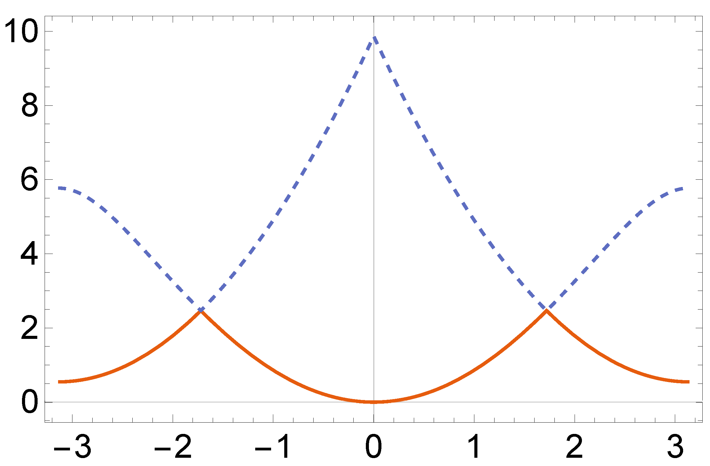
$t_2=\sqrt{2}/2$. In this case,

$${\eta }_{\pm }^{\gamma }(\lambda ,\theta )=\pm \frac{1}{2}\pm \frac{cos{\theta }_1}{2},$$

(41)

with parabolic touches occurring at ${\theta }_1\pm \pi$, with value ${\eta }_{\pm }^{\gamma }(\lambda ,{\theta }_1)=0$, which proves that the dispersion relation of $H^{\gamma }$ does not have any Dirac cones (see Figure 5b).

(iii)

$\sqrt{2}/2<t_2<1$. Differently from the cases (i) and (ii), the Dirac cones are present in this situation. In fact, we have that ${\eta }_{+}^{\gamma }(\lambda ,\theta )={\eta }_{-}^{\gamma }(\lambda ,\theta )=0$ if, and only if, ${\theta }_1=\pm {\theta }_1^D$, with ${\theta }_1^D=arccos(-\frac{1}{2t_2^2})$. Expanding ${\eta }_{\pm }^{\gamma }(\lambda ,\theta )$ around $\pm {\theta }_1^D$, in the analogous way we have done in the $\beta$-graphyne case, we obtain

$${\eta }_{\pm }^{\gamma }(\lambda ,\theta )-{\eta }_{\pm }^{\gamma }(\lambda ,{\theta }_D)=\pm {\tilde{\gamma }}^{\gamma }|\theta -{\theta }_D|-\mathcal{O}\left(|\theta -{\theta }_D{|}^2\right),$$

(42)

with ${\theta }_D=({\theta }_1^D,-{\theta }_1^D)$ and

$${\tilde{\gamma }}^{\gamma }=\frac{\sqrt{4t_2^4-1}}{1+2t_2^2}>0.$$

(43)

Analogously, one deals with $-{\theta }_D$. Combining (27) and (42), we obtain

$$\lambda \left(\theta \right)-\lambda \left({\theta }_D\right)=\pm {\overline{\gamma }}^{\gamma }|\theta -{\theta }_D|+\mathcal{O}\left(|\theta -{\theta }_D{|}^2\right)+\mathcal{O}\left({(\lambda \left(\theta \right)-\lambda \left({\theta }_D\right))}^2\right),$$

with ${\overline{\gamma }}^{\gamma }={\tilde{\gamma }}^{\gamma }/c\left({\theta }_D\right)$. Note that the $\overline{\gamma }$ is the linear coefficient, while the upper index “$\gamma$” indicates that we are considering the $\gamma$-graphyne. Therefore, for this parameter range, the dispersion relation of the $\gamma$-graphyne operator $H^{\gamma }$ has Dirac cones in its dispersion relation (see Figure 5c).

By analyzing the computational 3D plot of the dispersion relation, it was observed that the Dirac cones of the $H^{\gamma }$ is similar to the $\beta$-graphyne case, i.e., the Dirac cones are also situated at the vertices of a hexagon.

• $(6,6,12)$-graphyne

In the case of $(6,6,12)$-graphyne (see Figure 1d), the proposed parameter relations are $t_1=t_2=1$ and $0<t_3<1$. Hence,

$${\eta }_{\pm }^{(6,6,12)}(\lambda ,\theta )=\pm \frac{\sqrt{f\left(\theta \right)}}{2+t_3^2},$$

(44)

with

$$f\left(\theta \right)=f^{(6,6,12)}\left(\theta \right)=2+t_3^4+2cos{\theta }_1+2t_3^2\left(cos{\theta }_2+cos({\theta }_1-{\theta }_2)\right).$$

(45)

This case is tricker than the previous ones; in $\beta$- and $\gamma$-graphynes, we have taken the restriction to the segment $B_{\mathrm{d}}$ in the Brillouin zone, since it was observed that the (possible) Dirac cones were present in the diagonal ${\theta }_2=-{\theta }_1$. However, this does not happen for $(6,6,12)$-graphyne; we have found that the two Dirac points occur at the line

$${\theta }_2=r\left({\theta }_1\right):=(h(\ell )/\ell ){\theta }_1,$$

with $\ell =arccos\left(\frac{t_3^4-2}{2}\right)$ and

$$h\left(z\right):=z-arcsin\left(\frac{1}{t_3^2}sinz\right)-\pi .$$

(46)

Thus, let $B_r$ be the following restriction of the Brillouin zone B:

$$B_r:=\{\theta \in B:{\theta }_2=r\left({\theta }_1\right)\}.$$

(47)

We shall check now that the points

$${\theta }_D^{+}:=(\ell ,h(\ell ))\mathrm{and}{\theta }_D^{-}=(-\ell ,h(-\ell )),$$

in $B_r$, are D-points. Let $\theta \in B_r$. Expanding $f\left(\theta \right)$ around ℓ, we obtain

$$\begin{array}{}\mathrm{(48)}& f\left(\theta \right)= f(\ell )+f^{\prime }(\ell )({\theta }_1-\ell )+\frac{f^{\prime \prime }(\ell )}{2}{({\theta }_1-\ell )}^2+\mathcal{O}\left({({\theta }_1-\ell )}^3\right)\hfill \mathrm{(49)}& \hspace{1em} = \frac{f^{\prime \prime }(\ell )}{2}{({\theta }_1-\ell )}^2+\mathcal{O}\left({({\theta }_1-\ell )}^3\right),\hfill \end{array}$$

since $f(\ell )=f^{\prime }(\ell )=0$, with $f^{\prime }$ meaning the derivative of f with respect to ${\theta }_1$. It implies that

$${\eta }_{\pm }^{(6,6,12)}(\lambda ,\theta )-{\eta }_{\pm }^{(6,6,12)}(\lambda ,\ell )=\pm {\tilde{\gamma }}^{(6,6,12)}|\theta -{\theta }_D^{+}|+\mathcal{O}\left({({\theta }_1-\ell )}^2\right),$$

(50)

with ${\tilde{\gamma }}^{(6,6,12)}=\sqrt{f^{\prime \prime }(\ell )}/\left(\sqrt{2}(2+t_3^2)\right)$. Combining (50) and (27), we obtain

$$\lambda \left(\theta \right)-\lambda \left({\theta }_D^{+}\right)={\gamma }^{(6,6,12)}|\theta -{\theta }_D^{+}|+\mathcal{O}\left(|\theta -{\theta }_D^{+}{|}^2\right)+\mathcal{O}\left({(\lambda \left(\theta \right)-\lambda \left({\theta }_D^{+}\right))}^2\right),$$

with

$${\gamma }^{(6,6,12)}=\frac{{\tilde{\gamma }}^{(6,6,12)}}{c\left({\theta }_D^{+}\right)},{\theta }_D^{+}=(\ell ,h(\ell )).$$

Analogously, one deals with ${\theta }_D^{-}$.

Therefore, the dispersion relation of the $(6,6,12)$-graphyne operator $H^{(6,6,12)}$ has Dirac cones on the Brillouin zone (Figure 6), as found in [9] via a tight-binding model and in [14] via first principles calculations, and here for all allowed parameter values.

Differently from the $\beta$- and $\gamma$-graphyne, which the Dirac cones are situated at the vertices of a hexagon, the Dirac cones of the dispersion relation of $(6,6,12)$-graphyne occurs at the vertices of a rhombus. In a similar way, one checks that the other two Dirac cones occuring at the D-points are $\pm {\overline{\theta }}_D$, with ${\overline{\theta }}_D=(\overline{\ell },\overline{\ell }/2)$ and $\overline{\ell }=arccos\left(-(2-t_3^4)/2\right)$.

5. Graphyne Nanotubes

5.1. Spectra of Graphyne Nanotubes

Let $p=(p_1,p_2)\in {\mathbb{Z}}^2\setminus \left\{0\right\}$ be a vector of the lattice of translation symmetries of the graph G, denoting the corresponding nanotube by $G_p=G_{(p_1,p_2)}$ and the graphyne nanotube operator $H_p=H_{(p_1,p_2)}$, as defined at the end of Section 2.

As in Section 3, we apply the Floquet–Bloch theory that provides the Bloch Hamiltonian operators $H_p\left(\theta \right)$ for each quasimomentum $\theta$ in the Brillouin zone B and the decomposition

$$\sigma \left(H_p\right)=\bigcup _{\theta \in B}{H}_p\left(\theta \right),$$

(51)

with $\sigma \left(H_p\left(\theta \right)\right)={\left\{{\lambda }_{p,n}\left(\theta \right)\right\}}_n$, purely discrete. Since a function u on $G_p$ lifts to a p-periodic function on G, that is,

$$u(x+p_1{E}_1+p_2{E}_2)=u\left(x\right),$$

then, by the Floquet condition (6), it follows that

$$p·\theta =p_1{\theta }_1+p_2{\theta }_2\in 2\pi \mathbb{Z}.$$

(52)

Hence, we consider the restriction $B_p\subset B$ of the Brillouin zone given by

$$B_p=\{\theta \in B:p·\theta \in 2\pi \mathbb{Z}\}.$$

(53)

Therefore, (51) turns into

$$\sigma \left(H_p\right)=\bigcup _{\theta \in B_p}{H}_p\left(\theta \right),$$

(54)

and the dispersion relation for $H_p$ is just the dispersion relation of H (see Section 3) restricted to $B_p$, that is, it is given by

$$D\left(\lambda \right)=\pm \frac{2\sqrt{f\left(\theta \right)}}{T},\lambda \notin \sigma \left(H^D\right),\theta \in B_p,$$

(55)

where $D\left(\lambda \right)=cos\left(\sqrt{\lambda }\right)$ (see (23)), $f\left(\theta \right)=F\left(\theta \right)\overline{F}\left(\theta \right)$, $F\left(\theta \right)=t_1^2+t_2^2{e}^{i{\theta }_1}+t_3^2{e}^{i{\theta }_2}$ and $T=t_1^2+t_2^2+t_3^2$.

5.2. Dirac Cones

Now, we analyze the possible presence of Dirac cones in the dispersion relation (55) of the graphyne nanotube operator $H_p$. As before, we analyze separately the $\beta$, $\gamma$ and $(6,6,12)$-graphyne.

Let ${\theta }_D\in B$ be a D-point of the graphyne operator H (see (24)). Since the dispersion relation of $H_p$ is the dispersion relation of H restricted to $B_p$, then ${\theta }_D$ is a D-point of the nanotube graphyne operator $H_p$ if, and only if, ${\theta }_D$ belongs to the restriction $B_p$. Thus, given the D-point ${\theta }_D$ in each case of graphyne, we determine p in order to have ${\theta }_D\in B_p$.

• $\beta$-graphyne nanotube

As discussed in Section 4, the dispersion relation of the $\beta$-graphyne operator $H^{\beta }$ has D-points at $\pm {\theta }_D$, with

$${\theta }_D=({\theta }_1^D,-{\theta }_1^D),{\theta }_1^D=arccos(t_1^2/2)-\pi .$$

(56)

Hence, the condition for ${\theta }_D\in B_p$ reduces to (similarly for $-{\theta }_D$)

$$\begin{array}{ccc}\hfill p·{\theta }_D& =& p_1·{\theta }_1^D-p_2·{\theta }_1^D\hfill \\ & =& arccos(t_1^2/2)(p_1-p_2)+\pi (p_1-p_2)\in 2\pi \mathbb{Z}.\hfill \end{array}$$

The above condition implies that the difference $p_1-p_2$ must be an even integer, that is, $p_1-p_2=2q$, with $q\in \mathbb{Z}$. Then,

$$arccos(t_1^2/2)(p_1-p_2)=2arccos(t_1^2/2)q=2\pi r,r\in \mathbb{Z},$$

that is,

$$t_1^2=2cos\left(\frac{r}{q}\pi \right),r,q\in \mathbb{Z}.$$

(57)

Because of the parameter $t_1\in (0,1)$, we have $0<2cos(r\pi /q)<1$. Let the function

$$g^{\beta }\left(x\right):=2cos\left(\pi x\right).$$

(58)

It is easy to see that $0<g^{\beta }\left(x\right)<1$ if, and only if, $x\in C^{\beta }$, with

$$C^{\beta }:=\bigcup _{n\in \mathbb{N}\cup \left\{0\right\}}(J_n^{+}\cup J_n^{-}),$$

$$J_n^{+}=\left\{\begin{array}{c}\left(\frac{1}{3}+n,\frac{1}{2}+n\right),n\mathrm{even}\hfill \\ \left(\frac{1}{2}+n,\frac{2}{3}+n\right),n\mathrm{odd}\hfill \end{array}\right.J_n^{-}=\left\{\begin{array}{c}\left(-\frac{1}{2}-n,-\frac{1}{3}-n\right),n\mathrm{even}\hfill \\ \left(-\frac{2}{3}-n,-\frac{1}{3}-n\right),n\mathrm{odd}\hfill \end{array}\right..$$

Hence, $t_1\in (0,1)$ if, and only if, $r\pi /q\in C^{\beta }$. For instance, if $p=(p_1,p_2)$ is such that $p_1-p_2=14$, then if $r=1$ and $q=7$, it follows that $r\pi /q=\pi /7\in J_0^{+}$, which implies that $0<t_1^2=2cos(\pi /7)<1$ (and so $t_1\in (0,1)$) and, thus, $p·{\theta }_D\in 2\pi \mathbb{Z}$.

Therefore, $\pm {\theta }_D$ are D-points of the dispersion relation of the $\beta$-graphyne nanotube operator $H_p^{\beta }$, for $p=(p_1,p_2)$, if, and only if, there exists $r,q\in \mathbb{Z}$, such that $p_1-p_2=2q$ and $r\pi /q\in C^{\beta }$.

• $\gamma$-graphyne nanotube

From Section 4, we know that $\pm {\theta }_D$, with ${\theta }_D=({\theta }_1^D,-{\theta }_1^D)$, ${\theta }_1^D=arccos(-1/2t_2^2)$, are D-points of $\gamma$-graphyne operator $H^{\gamma }$ if $\sqrt{2}/2<t_2<1$. Hence, given $p=(p_1,p_2)\in {\mathbb{Z}}^2$, then $\pm {\theta }_D$ are D-points of $H_p^{\gamma }$ if, and only if, $p·(\pm {\theta }_D)\in B_p$. By following the steps in the discussion of the $\beta$-graphyne nanotube case, we obtain that

$$t_2^2=-\frac{1}{2cos\left(\frac{r}{q}\pi \right)},$$

(59)

with $r,q\in \mathbb{Z}$ and $p_1-p_2=2q$. Let

$$g^{\gamma }\left(x\right):=\sqrt{-1/2cos\left(\pi x\right)}.$$

Then, it follows that $\sqrt{2}/2<g^{\gamma }\left(x\right)<1$ if, and only if, $x\in C^{\gamma }$, with $C^{\gamma }={\bigcup }_{n\in \mathbb{Z}}{J}_n$, n odd and $J_n=(n-1/3,n+1/3)$. For instance, if p is such that $p_1-p_2=6$, then for $r=1$ and $q=3$, it follows that $r\pi /q=\pi /3\in J_1$ and, then $t_2\in (\sqrt{2}/2,1)$.

Therefore, for $t_2\in (\sqrt{2}/2,1)$, $\pm {\theta }_D$ are D-points of the dispersion relation of the $\gamma$-graphyne nanotube operator $H_p^{\gamma }$, for $p=(p_1,p_2)$, if, and only if, there exists $r,q\in \mathbb{Z}$, such that $p_1-p_2=2q$ and $r\pi /q\in C^{\gamma }$.

If $t_2=\sqrt{2}/2$, we have found that the dispersion relation of $H^{\gamma }$ has parabolic touches at $\pm (\pi ,-\pi )$. By imposing the restriction $B_p$ to these points, we obtain that $p_1-p_2$ must be even. Thus, if $p=(p_1,p_2)$ is such that $p_1-p_2=2q$, $q\in \mathbb{Z}$, then it follows that the dispersion relation of $H_p^{\gamma }$ has parabolic touches at $\pm (\pi ,-\pi )$.

• $(6,6,12)$-graphyne nanotube

We have found in Section 4 that, for $t_3\in (0,1)$,

$${\theta }_D^{\pm }=(\pm \ell ,h(\pm \ell )),$$

with $\ell =arccos\left(\frac{t_3^4-2}{2}\right)$ and $h\left(z\right)=z-arcsin\left(\frac{1}{t_3^2}sinz\right)-\pi$, which are D-points for $H_p^{(6,6,12)}$. Due to the complexity of the function $h\left(x\right)$ and the value of ℓ, we were just able to (analytically) analyze the possible presence of Dirac cones in the dispersion relation of the zig-zag nanotubes $G_p^{(6,6,12)}$, with $p=(N,0)$ and $N\in \mathbb{Z}$. By imposing that ${\theta }_D^{\pm }\in B_p$ and following the steps of $\beta$-graphyne case, we obtain

$$t_3^2=\sqrt{2cos\left(\frac{q}{N}2\pi \right)+2},q\in \mathbb{Z}.$$

(60)

Hence, $t_3\in (0,1)$ if, and only if, $2q\pi /N\in C^{(6,6,12)}$, with

$$C^{(6,6,12)}=\bigcup _{n\in \mathbb{Z}}{J}_n,J_n=\left(\frac{n}{2}-\frac{1}{6},\frac{n}{2}+\frac{1}{6}\right),n\mathrm{odd}.$$

Therefore, ${\theta }_D^{\pm }$ are D-points for the zig-zag nanotube $C_{(N,0)}^{(6,6,12)}$ if, and only if, there exists $q\in \mathbb{Z}$ such that $2q\pi /N\in C^{(6,6,12)}$.

6. Summary and Conclusions

In some situations, like graphene, QGMs are useful as models that usually permit an analytical approach with explicit calculations. For a single graphene sheet, it was mainly developed in [4,5] and has become standard, but requires that all graph edges have the same length; it was also applied to a particular equilateral graphyne in [15]. Motivated by previous works on multilayer graphene [6,7], the present authors have suggested some adaptations (1) in the boundary conditions, (2) selection of graphyne edges and (3) heuristic choices of parameters that take into account the intensity of chemical bonds, which have permitted an effective graph modeling of some graphynes.

We have proposed QGMs of the graphynes discussed in [9,14], in order to investigate Dirac cones; the main differences to graphene are that usually their hexagonal structure have edges of different lengths which carry different chemical bonds (in each graphyne, there are two or three types of bonds that repeat periodically). In principle, it is not immediate how to model such situations via quantum graphs; hence, we had to make some hypotheses which were based on heuristic observations and ad hoc procedures. We have also discussed the presence of Dirac cones for the corresponding graphyne nanotubes.

Our general approach was to model through the honeycomb structure of graphene in all cases, but introducing a positive parameter for each edge: there are three parameters, corresponding to the three edge intensities in the associated fundamental domain W of the honeycomb lattice (see Figure 2b). The idea is that the stronger the bond in an edge, the more influence it should have on the boundary condition balance (see Equations (3) and (4)). Next, we have tried to propose a way to associate edges of the graphyne to the ones ($a_1,a_2,a_3$) of W; of course, the choice must be a triple that appears in the graphyne that is being considered, and the idea was to select the one that is more abundant in each graphyne fundamental domain (which are indicated in Figure 1). However, this is not the case of $(6,6,12)$-graphyne, as explained in previous sections. It was then recovered, via QGMs, results from tight-binding and first-principle calculations in the literature, although our results for the $\gamma$-graphyne present a transition from bands with a gap to bands with Dirac cones, as a parameter changes.

Our effective models pick the most influential three-edge structure of each graphyne and, also to simplify technical matters, some carbon bonds are considered to have similar strengths (and thus imply the same value of the corresponding parameters in (3) and (4)). For example, the QGM of graphene in the literature does not distinguish single and double carbon bonds, whose difference of enthalpies is 256 kJ/mol; thus, for each graphyne, we have associated the same parameter value to edges whose difference of enthalpies is “close” to such value. This is particularly important (and it was a guide) for the $\alpha$-graphyne, whose proposed QGM then coincides with the one of graphene.

It would be interesting whether the found transition in $\gamma$-graphyne could be replicated either experimentally or by varying parameters in other theoretical calculations (e.g., tight-binding ones). We finish by mentioning that our proposal, to adapt QGMs to some graphynes, is a combination of heuristics, effective models and, after modeling, our results are mathematically rigorous.

References

- Castro Neto, A.H.; Guinea, F.; Peres, N.M.R.; Novoselov, K.S.; Geim, A.K. The electronic properties of graphene. Rev. Mod. Phys. 2014, 81, 109–162. [Google Scholar] [CrossRef] [Green Version]
- Fefferman, C.L.; Weinstein, M.I. Honeycomb lattice potentials and Dirac cones. J. Am. Math. Soc. 2012, 25, 1169–1220. [Google Scholar] [CrossRef] [Green Version]
- Berkolaiko, G.; Comech, A. Symmetry and Dirac points in graphene spectrum. J. Spectr. Theory 2018, 8, 1099–1147. [Google Scholar] [CrossRef] [Green Version]
- Amovilli, C.; Leys, F.; March, N. Electronic energy spectrum of two-dimensional solids and a chain of C atoms from a quantum network model. J. Math. Chem. 2004, 36, 93–112. [Google Scholar] [CrossRef]
- Kuchment, P.; Post, O. On the spectra of carbon nano-structures. Commun. Math. Phys. 2007, 275, 805–826. [Google Scholar] [CrossRef] [Green Version]
- de Oliveira, C.R.; Rocha, V.L. Dirac cones for bi- and trilayer Bernal-stacked graphene in a quantum graph model. J. Phys. A Math. Theor. 2020, 53, 505201. [Google Scholar] [CrossRef]
- de Oliveira, C.R.; Rocha, V.L. From multilayer AA-stacked graphene sheets to graphite: Graph models and Dirac cone. Z. Naturforsch. A 2021, 76, 371–384. [Google Scholar] [CrossRef]
- de Oliveira, C.R.; Rocha, V.L.; Souza, O.N. Boron nitride and graphene heterostructures modeled by quantum graphs. (preprint, submitted for publication).
- Liu, Z.; Yu, G.; Yao, H.; Liu, L.; Jiang, L.; Zheng, Y. A simple tight-binding model for typical graphyne structures. New J. Phys. 2012, 14, 113007. [Google Scholar] [CrossRef] [PubMed] [Green Version]
- Baughman, R.H.; Eckhardt, H. Structure–property predictions for new planar forms of carbon: Layered phases containing sp2 and sp atoms. J. Chem. Phys. 1987, 87, 6687–6699. [Google Scholar] [CrossRef]
- Desyatkin, V.G.; Martin, W.B.; Aliev, A.E.; Chapman, N.E.; Fonseca, A.F.; Galvão, D.S.; Miller, E.R.; Stone, K.H.; Wang, Z.; Zakhidov, D.; et al. Scalable synthesis and characterization of multilayer γ-graphyne, new carbon crystals with a small direct band gap. J. Am. Chem. Soc. 2022, 144, 17999–18008. [Google Scholar] [CrossRef] [PubMed]
- Kang, J.; Wei, Z.; Li, J. Graphyne and its family: Recent theoretical advances. Acs Appl. Mater. Interfaces 2019, 11, 2692–2706. [Google Scholar] [CrossRef] [PubMed]
- Rawat, S. Graphene is a Nobel Prize-Winning “Wonder Material” Graphyne Might Replace it. Big Think. The Future, 5 August 2022. Available online: https://bigthink.com/the-future/graphyne/ (accessed on 12 May 2023).
- Malko, D.; Neiss, C.; Viñes, F.; Görling, A. Competition for graphene: Graphynes with direction-dependent Dirac cones. Phys. Rev. Lett. 2012, 108, 086804. [Google Scholar] [CrossRef] [PubMed] [Green Version]
- Do, N.T.; Kuchment, P. Quantum graph spectra of a graphyne structure. Nanoscale Syst. Math. Model. Theory Appl. 2013, 2, 107–123. [Google Scholar] [CrossRef]
- Enyanshin, A.; Ivanovskii, A. Graphene alloptropes: Stability, structural and electronic properties from DF-TB calculations. Phys. Status Solidi (b) 2011, 248, 1879–1883. [Google Scholar]
- Harris, P. Carbon Nano-Tubes and Related Structures; Cambridge University Press: Cambridge, UK, 2002. [Google Scholar]
- Brown, M.B.; Eastham, M.S.P.; Schmidt, K.M. Periodic Differential Operators; Birkhäuser: Basel, Switzerland, 2013. [Google Scholar]
- Eastham, M.S.P. The Spectral Theory of Periodic Differential Equations; Scottish Acad. Press: Edinburgh/London, UK, 1973. [Google Scholar]
- Kuchment, P. Floquet Theory for Partial Differential Equations; Birkhäuser: New York, NY, USA, 1993. [Google Scholar]
- Reed, M.; Simon, B. Methods of Modern Mathematical Physics IV: Analysis of Operators; Academic Press: New York, NY, USA, 1978. [Google Scholar]
- Berkolaiko, G.; Kuchment, P. Introduction to Quantum Graphs; American Mathematical Society: Providence, RI, USA, 2012. [Google Scholar]
Disclaimer/Publisher’s Note: The statements, opinions and data contained in all publications are solely those of the individual author(s) and contributor(s) and not of MDPI and/or the editor(s). MDPI and/or the editor(s) disclaim responsibility for any injury to people or property resulting from any ideas, methods, instructions or products referred to in the content. |
© 2023 by the authors. Licensee MDPI, Basel, Switzerland. This article is an open access article distributed under the terms and conditions of the Creative Commons Attribution (CC BY) license (https://creativecommons.org/licenses/by/4.0/).
Share and Cite
de Oliveira, C.R.; Rocha, V.L. Effective Quantum Graph Models of Some Nonequilateral Graphyne Materials. C 2023, 9, 76. https://doi.org/10.3390/c9030076
de Oliveira CR, Rocha VL. Effective Quantum Graph Models of Some Nonequilateral Graphyne Materials. C. 2023; 9(3):76. https://doi.org/10.3390/c9030076
Chicago/Turabian Stylede Oliveira, César R., and Vinícius L. Rocha. 2023. "Effective Quantum Graph Models of Some Nonequilateral Graphyne Materials" C 9, no. 3: 76. https://doi.org/10.3390/c9030076