Abstract
The differentiation of clones within grape cultivars, specifically Vitis vinifera, has significant potential for the wine industry. This differentiation involves associating morphological features or a genetic signature with a particular cultivar clone, which is a challenging task. It has been difficult to experimentally find genetic signatures that differentiate a pair of clones, despite evidence suggesting that genomic differences exist. Are there genetic or genomic differences in a pair of clones? If so, where are the variations in the genome? Are there variations in protein coding genes? We addressed these questions by performing a bioinformatic analysis to identify genetic differences between certified clones of the same cultivar. Utilising genome sequencing data from tissue samples, we identified genomic positions differing between the clones and their cultivar reference genome, meeting the filtering criteria. Applying this approach to the Carménère and Merlot clones resulted in 5718 and 5218 variations, respectively, that differentiated the clones. Visual validation of 50 variations per cultivar revealed that 12% of these variations were located in the Merlot genes, while 32% were found in the Carménère genes. We estimated between 600 and 1000 variations per cultivar that could be validated by visual inspection. Despite the presence of these variations within genes, none was found to have a disruptive effect on protein function. By comparing our results with those of previous studies, we discuss issues pertaining to clone differentiation. In conclusion, there are genomic variations in pairs of clones that allow for their differentiation, though the variations are not directly related to the phenotype.
1. Introduction
The International Organization of Vine and Wine (OIV) defines a clone as the vegetative offspring of a single plant. For selection purposes, this unique plant is chosen based on its varietal identity, phenotypic traits, and overall health. The mechanisms responsible for clonal differences may include changes in diseases such as viruses, epigenetic differences, genetic mutations, or various combinations of these effects [1].
The process of obtaining clonal selections involves both phenotypic and genetic techniques, along with vegetative propagation methods. Initially, plants are selected in the field based on their disease resistance, yield, and fruit quality. These selected individuals are then vegetatively propagated through methods such as grafting and cuttings. During this process, a detailed phenotypic of the clones is conducted using chemical and sensory analysis techniques to assess their oenological attributes according to OIV standards. This process can take several years, depending on phenotypic and genetic evaluations and the vegetative propagation cycles. It is often more than 10 years before the clones become commercially available.
The need to identify clones arises from challenges faced by the wine industry, such as clone differentiation before propagation. Significant concerns have been raised regarding which clone is being propagated and the time it takes to confirm the clone’s identity during cultivation. Although phenotypic analysis and molecular markers have been explored for clone identification, they have not been successful [2,3,4,5,6]. It is suggested that clones arise from the accumulation of somatic mutations that eventually affect the phenotype.
Research on genetic variability and clone differentiation has primarily focused on molecular markers. Among those effective for measuring clone variability within the same cultivar are Simple Sequence Repeats (SSRs), Amplified Fragment Length Polymorphisms (AFLPs), and Random Amplified Polymorphic DNA (RAPD) markers. While AFLP and RAPD markers have yielded good results, SSR markers have become the focus since the early 2000s due to their PCR-derived, codominant, polymorphic nature, making them valuable for genetic analysis in heterozygous species [7]. However, while SSR markers have been established for cultivar identification, they have not succeeded in clone identification [3,5,6]. Furthermore, developing new SSR markers is both labour intensive and costly.
Currently, whole-genome sequencing (WGS) analyses are used to identify millions of mutated positions, such as single nucleotide variations (SNVs), single nucleotide polymorphisms (SNPs), and structural variations (SVs). Over the past two decades, WGS has become more reliable, accessible, and cost-effective. The WGS data could potentially aid in clone identification or differentiation [8,9,10]. However, clone identification through genome sequencing is a comparative task, as a clone can only be identified relative to other clones. Due to the limited availability of public WGS data on Vitis vinifera clones, universal clone identification using WGS is not currently feasible. Nonetheless, differentiating a pair of clones using WGS represents progress, even if the variations found do not universally characterise the certified clones. Identifying local genomic differences to distinguish a pair of clones using WGS is a crucial first step.
In this study, we present the genome-wide differentiation of a pair of certified clonal selections from two cultivars, Carménère and Merlot, grown in Chile by Viña Concha y Toro. Our goal was to determine if and where genetic differences between clones of the same cultivar were located, evaluate these differences at a functional level, and assess whether they were associated with relevant metabolic pathways in grapevines.
2. Materials and Methods
2.1. Experiments
2.1.1. DNA Extraction
Plant material was collected from the leaves of four clonal selections. The Carménère clonal selections in this study included Clone 1235 and internal Clone 39 from Mercier Nursery, distinguished by their enhanced vigour compared to other Carménère clones. The Merlot clones, Clone 181 and Clone 348, mainly differed in bunch weight and berry sugar content.
Ten leaves were collected from each plant, with three biological samples taken for each clonal selection. We designated these clonal selections as Clone 1 and Clone 2, with the biological samples labelled with the suffixes “.1”, “.2”, and “.3”. Specifically, for Carménère, Clone 1 corresponded to Clone 1235, and Clone 2 to Clone 39. For Merlot, Clone 1 corresponded to Clone 348, and Clone 2 to Clone 181.
The DNA extraction from the grapevine leaves was performed using a Dneasy Plant Mini Kit (Qiagen, Hilden, Germany), following the manufacturer’s instructions. The DNA quantification was conducted using a Qubit 4.0 fluorometer (ThermoFisher, Waltham, MA, USA), with a dsDNA BR assay kit (SKU: Q32853, ThermoFisher, Waltham, MA, USA). The DNA integrity was evaluated using 0.8% agarose gels.
2.1.2. Library Construction and Sequencing
Genomic libraries for both clones were constructed using a TruSeq Nano DNA kit (Illumina, San Diego, CA, USA, SKU: 20015965), adhering to the manufacturer’s protocol. The quality of each library was assessed using a Fragment Analyser (Agilent, Santa Clara, CA, USA). The average fragment sizes were 300 bp and 265 bp for Clone 1 and Clone 2, respectively. The libraries were sequenced at Macrogen, Korea, using paired-end reads of 101 bp, in an Illumina HiSeq1500 sequencer.
The Carménère clone datasets were deposited in NCBI’s SRA Database under Bioproject PRJNA986085. The Merlot WGS datasets, previously registered in the SRA by another research group [9], were downloaded from the SRA Database (Bioproject PRJNA847341).
2.2. Bioinformatic Analyses
2.2.1. Quality Control and Trimming of Sequencing Reads
FastQC v. 0.11.9 [11] was used to assess the quality of the fastq files. The Carménère fastq files contained between 49 and 66 million paired-end reads, while the Merlot fastq files contained between 52 and 78 million paired-end reads. All samples had an average quality score above 28 on the Phred scale. The NCBI’s UNIVEC database was used to check for contamination in the read sets.
Despite the generally good quality of the reads, trimming was performed using Trimmomatic v. 3.16 [12] with the MAXINFO:40:0.9 module, applying a target length of 40 bp and strictness of 0.9. This approach balanced preserving read length while removing incorrect bases, with the 0.9 strictness prioritising accuracy. No reads were lost from any sample, but approximately 10% of the low-quality segments were removed. After trimming, the average quality of the fastq files increased to over 32 on the Phred scale, and more than 90% of the reads retained their original length of 101 bp.
2.2.2. Mapping Reads to the Reference Genome
The Carménère reference genome assembly and annotation for Clone 02—VCR702 v1.0 was downloaded from Cantu Lab’s Grape Genomics Database (http://www.grapegenomics.com/pages/VvCar/download.php, accessed on 8 September 2024). The Merlot reference assembly and annotation for Clone 15 v1.1 were also obtained from the Grape Genomics Database (http://www.grapegenomics.com/pages/VvMerl/download.php, accessed on 8 September 2024).
Processed reads were mapped to the reference genome assemblies using BWA v. 0.7.17-r1188 [13] with the mem option. After indexing the reference assemblies using the bwa index command with default parameters, the Carménère samples were aligned to the Carménère reference genome, and the Merlot sample reads were aligned to the Merlot reference genome. Only primary assemblies were used for both cultivars. The resulting SAM files were sorted by position, duplicate reads were flagged, and the SAM files were converted to BAM files and indexed using Samtools v. 1.11 [14].
2.2.3. SNP and InDel Calling
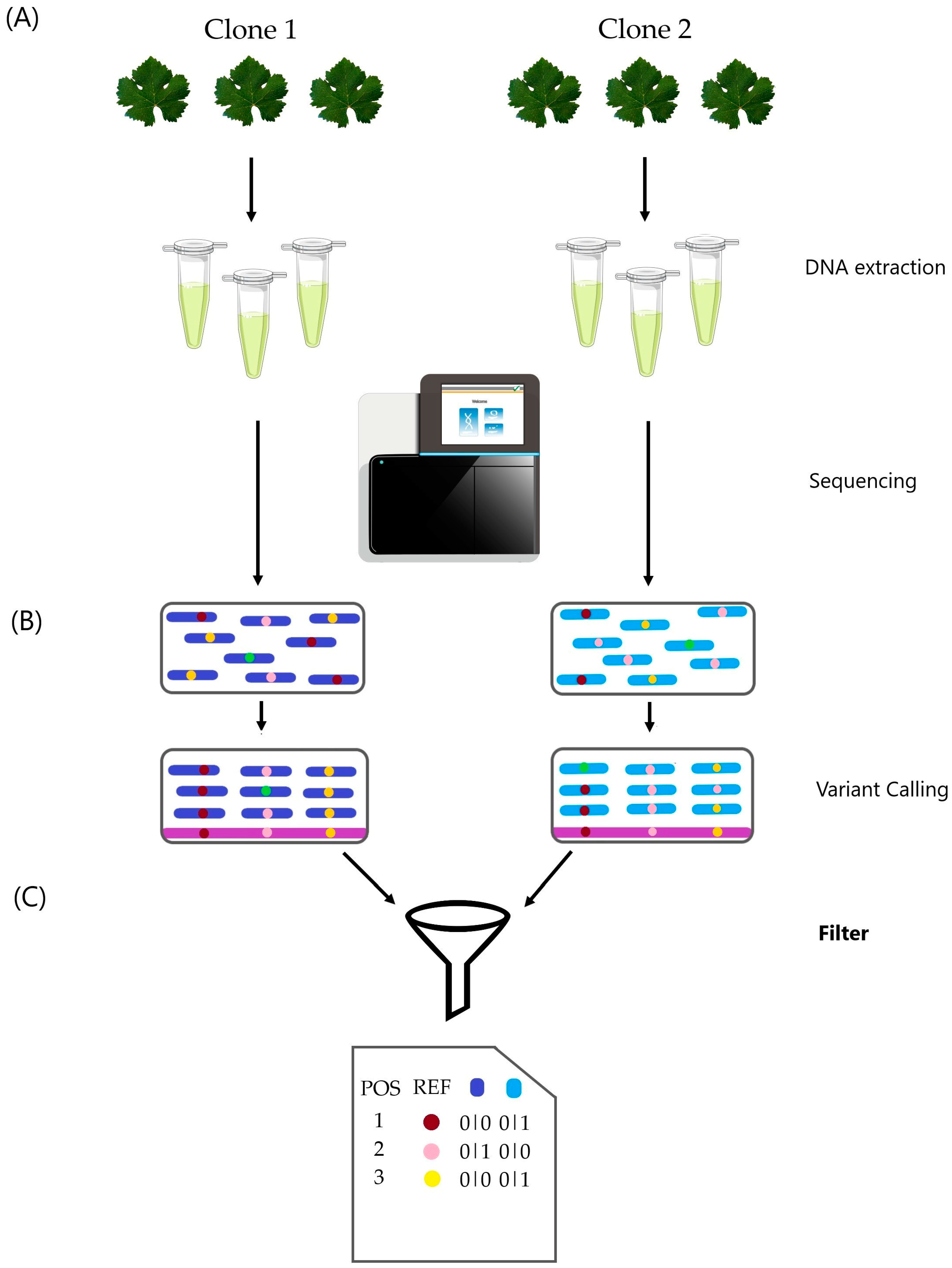
We identified variants following the methods illustrated in Figure 1. Single nucleotide polymorphisms (SNPs) and short insertions and deletions (InDels) smaller than 60 base pairs were culled using the Genome Analysis Toolkit (GATK) v. 4.2.3 [15]. The SNPs and InDels were detected simultaneously through local de novo assembly of haplotypes using the GATK HaplotypeCaller module for each sample. The resulting VCF files from all samples were merged into a single file using the GATK CombineGVCFs module. Joint genotyping was then performed on this combined input using the GATK GenotypeGVCFs tool, following the “Best Practice Workflows” available at the GATK Broad Institute website (https://gatk.broadinstitute.org, accessed on 8 September 2024).

Figure 1.
Clone differentiation flowchart. (A) DNA extraction and sequencing were performed on three biological samples per clone. (B) Variant calling analysis was conducted on the six samples following GATK best practice guidelines. (C) Final filtering steps considered filters such as biallelic sites, minor allele frequency (MAF), missing data, depth, genotype, and location within repetitive elements. Visual inspection of a sample of variations confirmed the results. “Filters” is in bold to highlight the importance of this step, as shown in the results.
2.2.3.1. Filters
From the VCF file obtained via GenotypeGVCFs, we selected sites where all samples showed the same genotype using BCFtools v. 0.1.16 [16] and AWK. Additional filtering criteria included minor allele frequencies (MAF) less than or equal to 10%; no missing data; variant quality scores below 100; and a read mean depth threshold of 18× for both cultivars. Variations located in repetitive regions were also excluded. Finally, we conducted a visual inspection of the reads alignment of each sample over the cultivar reference genome using the Integrative Genomics Viewer (IGV) v.2.12.3 software [17]. We selected the 25 variations with the lowest depths and the 25 variations with the highest depths. Variations that could differentiate the clones were selected based on the following criteria: the variation had to be visually validated in all three samples of one clone and absent in all samples of the other clone, or it had to be present in at least two samples of one clone and absent in all three samples of the other clone.
The final result was a list of genomic positions capable of differentiating the pair of clones.
A principal component analysis (PCA) and a hierarchical clustering, or tree, using as distance the proportion of loci that are different between clone samples (genetic distance), were carried out using the Adegenet package v. 2.1.10 [18] in R, to evaluate whether the identified variations could effectively distinguish Clone 2 from Clone 1 in each cultivar.
2.2.4. Annotations and Functional Effects of InDels and SNPs
To characterise and assess the functional impact of the previously identified variations, we determined their genomic locations, annotations, and effects on protein function.
The genome annotations, in GFF3 format, from the Carménère VCR 702 and Merlot clone 15 assemblies were used as references to locate the variations relative to the annotated genomic elements. To annotate these variations, we intersected the filtered VCF files with the corresponding GFF3 annotation files using the Bedtools intersect [19]. A variation was considered to be within a gene (or specific region) if 100% of the variation sequence was contained within that gene. Variations located in non-nuclear genomes were annotated using BLAST 2.5.0+ [20], aligning 1000 bp segments surrounding the variations to the Vitis vinifera mitochondrial and chloroplast genomes.
We used SnpEff v.5.0e [21] to annotate and assess the functional impact of the variations. SnpEff takes a VCF file (filtered in the previous section), the genome sequence, and the organism’s annotation as inputs. While SnpEff includes a default database with sequence and annotation information for model organisms, in this case, data were only available for Vitis vinifera PN40024. Therefore, we generated two new databases using the genome assemblies and annotation files for Carménère and Merlot. The output was a VCF file that included both the original annotations and the functional impacts of the variations. Additionally, SnpEff generates an HTML report detailing the type of variation (based on Sequence Ontology terms: http://sequenceontology.org, accessed on 8 September 2024), its impact, the affected region, variation length (in base pairs), and, for SNPs, the type of mutation (silent, missense, nonsense) and the codon-level changes it produces.
The SnpEff categorises the impact of variations into the following four levels: high, moderate, low, and modifier. High impact refers to variations that are likely to generate a truncated protein. Moderate impact indicates that the variation affects protein efficiency (non-synonymous mutation) without truncating it. Low impact refers to neutral changes (synonymous mutations). Modifier impact refers to variations that affect non-coding regions.
A supplementary file detailing the commands and computational programs used in this study is available (Supplementary Materials File S1).
3. Results
3.1. Variants Calling: Variations between Individuals vs. Variations That Differentiate Clones in Carménère and Merlot
3.1.1. Variant Calling of Carménère Clones
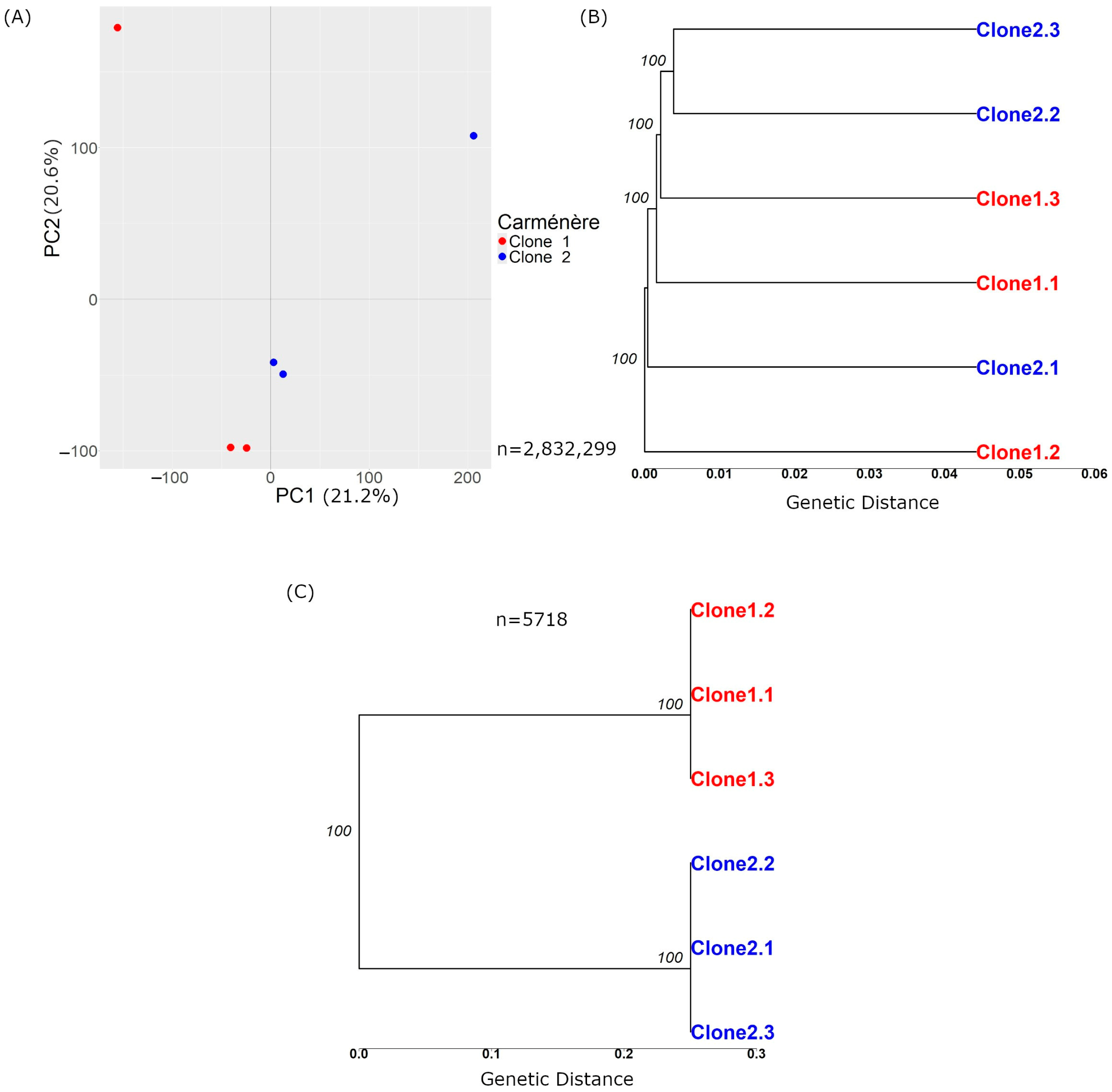
The variant calling process for samples from both clones resulted in 2,832,299 raw variations (Table 1). Of these, 2,053,007 were SNPs, 527,390 were insertions, and 284,793 were deletions. Figure 2A presents the principal component analysis (PCA), while Figure 2B shows a tree based on the genetic distance (the proportion of differing alleles between samples). In the PCA plot, the samples appeared intermixed rather than grouped by clone, indicating that the genetic variations did not separate the samples according to their clonal origin. Similarly, the tree showed minimal differences between samples, and these variations were insufficient to distinctly group the samples by clone.

Table 1.
Number of total variations resulting from the variant calling before and after applied filters; Number of variations assessed for visual validations and proportion of visually validated variations (50 variations/N° of variations assessed).
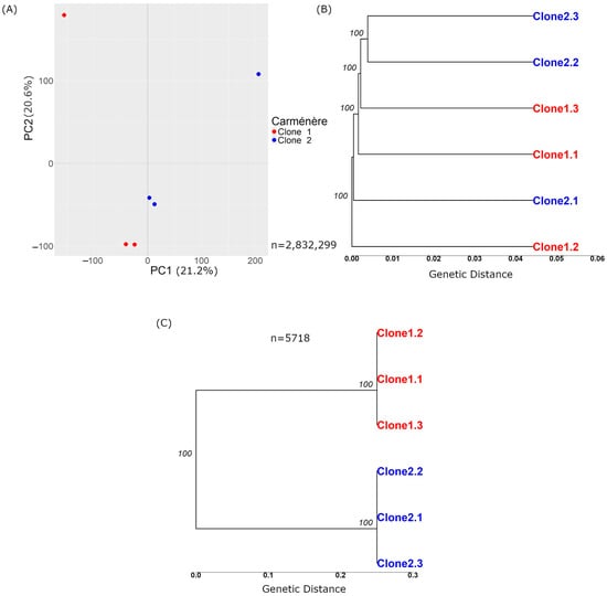
Figure 2.
Principal component analysis and tree based on genetic distance with Carménère variations before and after the filters. (A) and (B) show plots generated before applying the filters described in Section 2.2.3.1, based on n = 2,832,299 variations. (A) displays a PCA plot of the variant calls from the 6 Carménère samples, where the X-axis represents Principal Component 1, and the Y-axis represents Principal Component 2. The numbers next to each component indicate the variance explained by the data, which in this case is 21.2% for PC1 and 20.6% for PC2. (B) Tree based on genetic distance, with the numbers over the nodes representing branch support on a scale from 0 to 100. X-axis represents the genetic distance, indicating the proportion of differing sites among the samples. (C) Tree of Carménère clone samples after applying the filters from Section 2.2.3.1.
After applying the initial depth filter of 18×, the number of variations was reduced by 5.1%, leaving 2,688,957 variations. The minimal reduction in variations can be attributed to the high average depth of 71×, which was more than double the selected filter threshold. The peak variation occurred at 80×, which aligned with expectations, given that each sample had approximately 15× depth, resulting in a combined average depth of 90× across the six samples. Additionally, it is important to note that 1802 variations exhibited a depth exceeding 1000×. Subsequent application of the MAF, missing data, and minimum quality filters further reduced the variation count to 1,957,041.
At this stage, the remaining variations were still unable to differentiate between the clones due to many individual variations. To address this, we applied a genotype filter, which reduced the number of variations to 13,316. The purpose of filtering by genotype is to identify variations that are homozygous in one clone and heterozygous in the other. This process ensures that the samples possess one distinct allele, allowing for clear differentiation between the clones. Finally, by excluding variations located in repetitive elements, the total number of variations was further reduced to 5718 (Table 1).
It was not possible to perform PCA with the 5718 variations because the samples from the same clone shared identical genotypes and variations, while those between clones were different. This resulted in all the variance being captured by the first principal component, representing the differences between clones, leaving no second component to capture any variation within each clone. Figure 2C displays a tree wherein the scale of genetic distance differs from that in Figure 2B, highlighting the more pronounced differences in the analysed set of variations. This tree further demonstrated that the samples clustered by clone; all of the genetic differences occurred between clone types rather than within samples of the same clone.
To validate these variations, we conducted a visual inspection using the BAM alignment files in IGV. For Carménère, we reviewed 234 variations, visually validating the 25 with the lowest depth (18× or higher), followed by inspecting 174 variations to identify the 25 with the highest depth (20,620× or lower) (Table 1). This process involved the visual inspection of 50 variations, of which 21 met the criterion of being present in all three samples of one clone and absent in all three samples of the other clone. The remaining variations met the criterion of being present in two out of three samples and absent in the three samples of the other clone (or vice versa). Thus, it is estimated that around 12% of the predicted variations, 600, can be visually validated in the Carménère cultivar pair of clones.
3.1.2. Variant Calling of Merlot Clones
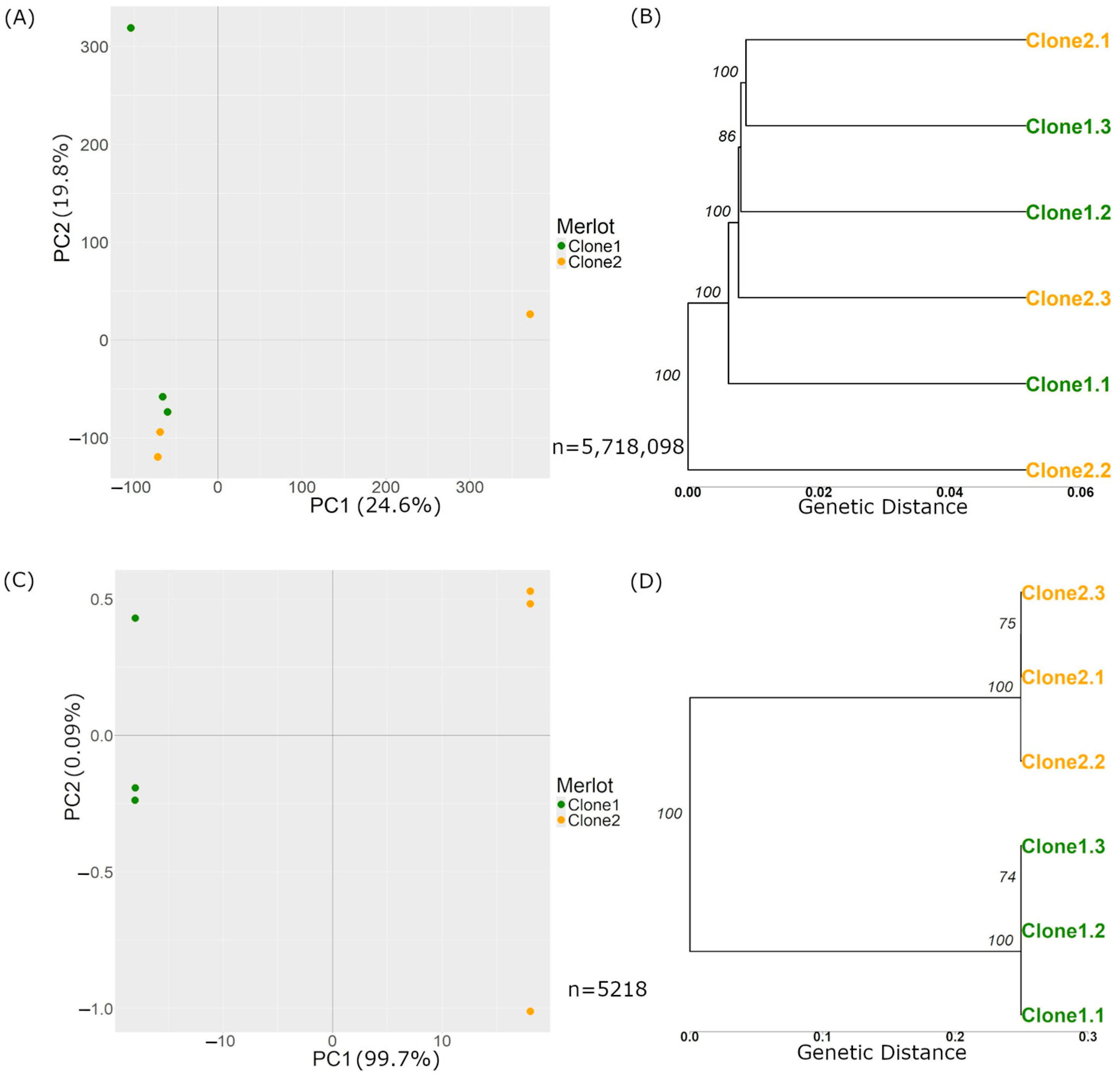
The variant calling process for both clones of Merlot with respect to the reference yielded 5,718,098 raw variants (Table 1), comprising 4,515,484 SNPs, 967,261 insertions, and 302,678 deletions. Figure 3A,B present a PCA and a genetic distance tree, respectively. In the PCA plot, the samples did not cluster by clone, indicating that genetic variations did not separate the samples according to clonal origin. Similarly to Carménère, the genetic distance tree revealed minimal differences between the samples that were insufficient for distinct clonal grouping.
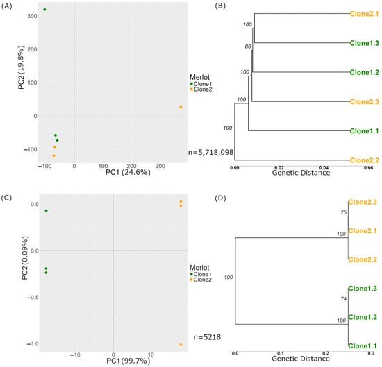
Figure 3.
PCAs and trees are based on genetic distance with Merlot variations before and after the filters. (A) and (B) show plots generated before applying the filters described in Section 2.2.3.1, based on n = 5,718,098 variations. (A) PCA plot of the variant calls from the 6 Merlot samples, where the X-axis represents Principal Component 1, and the Y-axis represents Principal Component 2. The numbers next to each component indicate the variance explained by the data, which in this case is 24.6% for PC1 and 19.8% for PC2. (B) Tree based on genetic distance, with the numbers over the nodes representing branch support on a scale from 0 to 100. The X-axis represents the genetic distance, indicating the proportion of differing sites among the samples. (C,D) show plots generated after applying the filters described in Section 2.2.3.1, based on n = 5218 variations (C) PCA plot of the variant calls where the X-axis represents PC 1, and the Y-axis represents PC 2. The numbers next to each component indicate the variance explained, which in this case is 99.7% for PC1 and 0.09% for PC2. (D) Tree of Merlot clone samples after filters.
After applying the minimum depth filter of 18×, the variant count was reduced to 5,625,624 variants. In the case of the Merlot clones, the average depth was 168×, which was nine times higher than the filter threshold. The maximum variant depth occurred at 170×, aligning with the expected average depth of 120× across the six samples, each with an approximate depth of 20×. Additionally, 16,808 variants exhibited depths exceeding 1000×. Further filtering based on MAF, missing data, and minimum quality reduced the variant count to 4,210,119.
Applying the genotype filter reduced the number of variations to 15,548. After further filtering those located in repetitive regions, the count decreased to 5218 (Table 1). We then conducted a PCA (Figure 3C). Along the X-axis, the samples were separated by clone, accounting for 99.7% of the variance in PC1. The PC2 revealed differences between the samples of the same clone, representing 0.07% of the variance. Figure 3D presents a genetic distances tree with a different genetic distance scale from Figure 3B, highlighting more pronounced differences in the analysed variant set. The tree demonstrated clear clustering by clone, with most genetic differences occurring between clone types rather than within samples of the same clone.
The same visual validation process used for Carménère was applied to Merlot. We reviewed 74 variations for Merlot, visually validating the 25 with the lowest depth (18× or higher), followed by the inspection of 170 variations to identify the 25 with the highest depth (1537× or lower) (Table 1). A total of 24 variations was present in all three samples of one clone and absent in all three samples of the other clone. The remaining variations were present in two out of three samples and absent in all three samples of the other clone (or vice versa). Thus, it is estimated that around 20% of the predicted variations, 1000, can be visually validated in the Merlot cultivar pair of clones.
3.2. Location of Variations within the Genome and Functional Impact on Transcriptional Sequences
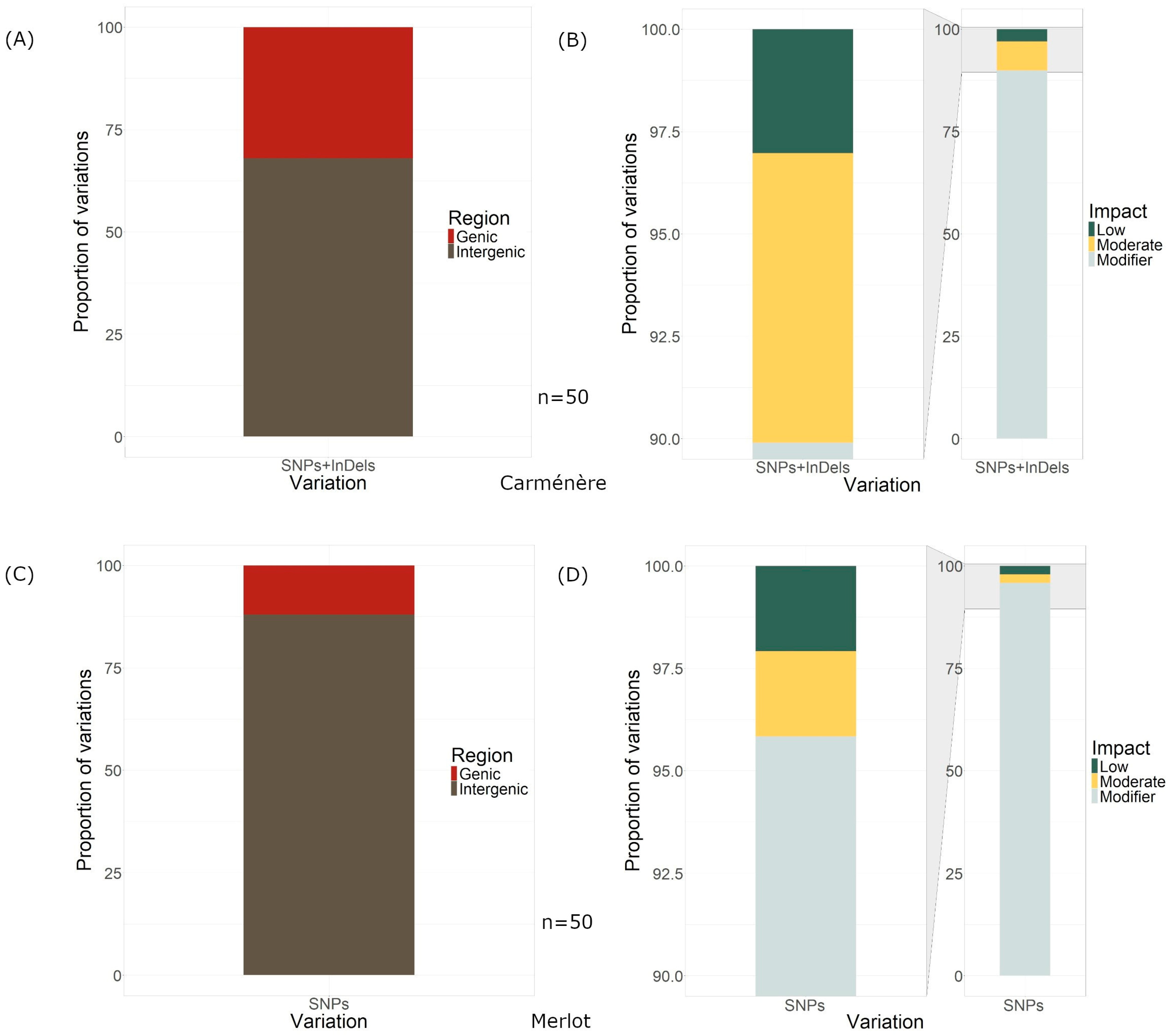
Regarding the location of the visually inspected variations in Carménère, 34 of the 50 variations were found within intergenic regions, while 16 were in genes (Figure 4A), and 10 were in exons. Regarding the location of the variations in the nuclear and non-nuclear genome, for Carménère, three variations out of the 50 found were in the mitochondrial genomes and one was in the chloroplast genome.
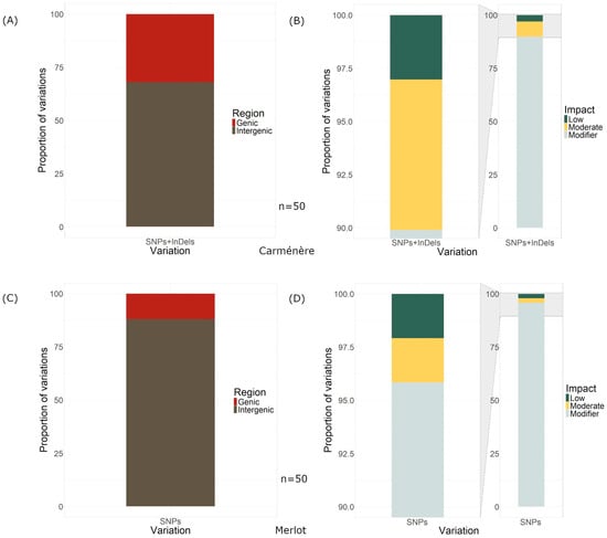
Figure 4.
Localization of the variations and their impact on the genome. (A) Region, genic or intergenic, of the variations on the Carménère genome. (B) Impact of the variations on the Carménère genome. (C) Region, genic or intergenic, of the variations on the Merlot genome. (D) Impact of the variations on the Merlot genome.
The SnpEff predicted 99 effects (low, modifier, and moderate) from all 50 variants that distinguished Clone 2 from Clone 1 in Carménère, of which only 3.03% were of low impact, while 89.899% of the effects were modifier effects and 7.071% were moderate (Figure 4B).
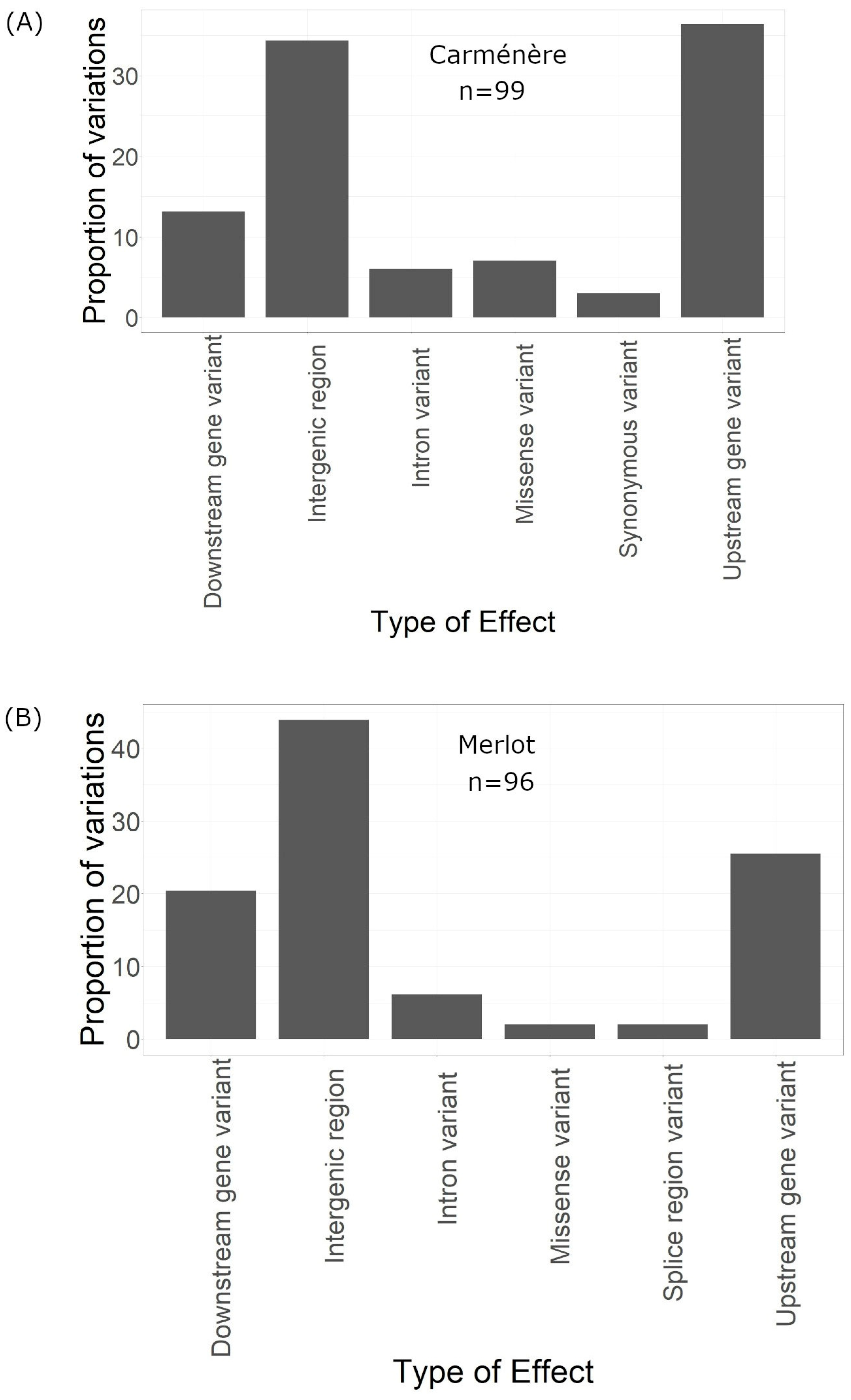
Of the 99 effects, 13 were classified as downstream gene variants, affecting regions downstream of genes, and another 39 were upstream variants. A total of 34 effects impacted intergenic regions, while six were located in intronic regions. Additionally, seven resulted in missense mutations, and three were synonymous (Figure 5A).

Figure 5.
Type of the effect of the variations in the genome. (A) Type of the effect of the variations of Carménère. (B) Type of the effect of the variations of Merlot.
Although missense variations were identified, SnpEff did not classify them as having a high impact, as they did not result in protein truncation. Overall, none of the 50 visually validated variations caused any truncation or disruption of proteins.
In Merlot, out of the 50 visually inspected variations, 44 were located in intergenic regions, 6 within genes, and 2 in exons (Figure 4C). Notably, no variations were detected in the mitochondrial or chloroplast genomes.
The SnpEFF predicted a total of 96 genome-wide effects resulting from these 50 variations. Among these effects, 2.083% were classified as low impact, 2.083% as moderate impact, and 95.833% as modifier impact (Figure 4D). The majority of the 96 effects were intergenic (43), while 20 were downstream, 25 were upstream, and 2 were missense variants (Figure 5B).
As with Carménère, although missense variations were present, none was classified as high impact, indicating that these variations did not negatively affect protein levels.
4. Discussion
4.1. Clonal Differentiation Method
4.1.1. Filters
The filtering step in our pipeline was crucial to reduce the over two million variations initially reported by GATK after aligning the sample clone reads to the reference genome of the cultivar. We established a minimum depth filter of 18× for three samples, based on the literature [22,23,24,25,26] that, through simulations and real data, allowed us to conclude that a final depth of 2× to 6× per sample was optimal for SNP calling. Including as many samples as possible was beneficial, as it increased the diversity of variations from the clone population [27]. The 18× depth filter is predicted to have a true-positive rate of over 95% for variations [26]. The GATK is estimated to recover approximately 86% of true-positive SNPs [28]. Despite these predictive values, visual inspection of the clone sample read alignments to the cultivar reference genome validated only about 12–20% (Merlot and Carménère, respectively) of the candidate variations resulting from the filtering step.
4.1.2. The Variations That Distinguished a Pair of Clones
Intravarietal genetic variability has been studied using various methodologies. Initially, researchers employed SSR [5,6], AFLP, and RAPDs [3] markers, and currently, they use SNPs [8,10], InDels [9], and SVs [1,9,29,30], taking advantage of the lower costs and increased accessibility of sequencing technologies for whole-genome studies.
The accessibility of whole-genome sequencing has opened up possibilities for identifying clonal markers, enabling the differentiation and identification of clonal selections [8,9,10]. The traditional markers mentioned earlier, such as SSR, AFLP, and RAPDs, were inadequate for achieving this goal.
In this work, the resulting set of variations that distinguished the two clones could not be used to universally characterise the clones. However, a subset of this number could, as the variations belonged, on average, to all the samples of each clone. The only way to determine the characteristic variations in each clone is to compare it with all other available clones. Therefore, until a sufficiently large number of genome sequences of all Carménère and Merlot clones is available, this method only allows for distinction between pairs of clones locally.
The tree results from the Merlot samples were similar to those obtained for the Carménère samples in terms of distinguishing the clones. In both cases, it was possible to group one of the clones and differentiate it from the samples of the other clone.
Although the initial number of variations identified in Carménère and Merlot differed significantly (2.8 million in Carménère and 5.7 million in Merlot), the final number of filtered variations was similar, with approximately 5000 for each cultivar. For Merlot, a larger number of individual variations was observed compared to Carménère, as evidenced by the nearly equivalent counts after the first filter of the genotype (13,000 for Carménère and 15,000 for Merlot). Notably, Merlot had nearly half the number of gene variations compared to Carménère. Despite Carménère having 32% of its variations within genes, none was classified as having high impact. Instead, they exhibited low or moderate impact, indicating that the variations are likely synonymous or missense variations, which suggests they may either alter protein efficiency or have no adverse effect on protein function. However, the second and third most frequent location of variation effects occurs in the upstream and downstream regions of protein-coding genes, respectively. We speculate that many of these variations may be associated with gene regulatory functions.
4.1.3. Limitations of Our Study
- Only two cultivars, only two clones per cultivar, and only three individuals or biological replicates per clone were used. As a preliminary study to find variations in clones, this may be considered the bare minimum amount of data to assess the variations. Despite using what could be considered the bare minimum, we found around 5000 variations per pair of clones per cultivar, out of which between 600 and 1000 variations (per cultivar) were estimated to be validated by visual inspection of the read alignments over the reference genome. However, more sequenced individuals [27] from a larger number of cultivars would be desirable and will be needed to confirm or improve our current estimations.
- Whole-genome sequencing of Vitis vinifera clones is an expensive and long-term enterprise. This study aimed to explore variations to see if a pair of clones can be differentiated through genomic variations. The next step is to look for patterns of variation in clones from different cultivars and find a cheaper and faster way of differentiating them.
- According to Ajay, 2011, the naïve approach of variant calling followed by the comparison of samples can often lead to errors [25,26]. As we used this exact approach, the filters step was crucial to obtain a more reliable group of candidate variations. In addition, visual inspection of these variations was necessary. In our case, the results of the visually validated variations, although estimated to be only between 12% (Carménère) and 20% (Merlot) of the total, confirmed the results of the pipeline for both cultivars.
- Additional filters can increase the number of variations that can differentiate a pair of clones. For example, Li remarked that one frequent source of errors in SNP calling is mismapped reads [25]. In our work, we considered all mapped reads, as opposed to considering only the uniquely mapped reads of the reference genome. Uniquely mapped reads might increase the number of variation candidates as a larger proportion of the sites would pass the biallelic sites filter, meaning the number of biallelic sites would increase after the multi-mapped reads were removed.
5. Conclusions
In this study, we explored the variations between a pair of clones in two Vitis cultivars, using a simple variant calling approach and applying a set of filters to reduce the number of false-positive candidates. After filtering, we visually inspected the results, further reducing the number of candidates. The results of this study can be summarized as follows:
- It was estimated that between 600 (for Carménère) and 1000 (for Merlot) SNPs can differentiate a pair of clones in the Carménère and Merlot cultivars of Vitis vinifera. Three deletions were visually validated in either cultivar.
- It was found that all visually validated variations had a homozygous genotype in one clone and a heterozygous genotype in the other, with one allele of the second clone matching that of the first clone.
- The proportion of SNPs located within genes versus intergenic regions was found to be 32% for Carménère and 12% for Merlot. All SNPs in gene regions were classified as having low, moderate, or modifier impacts, indicating that none of the identified variations was responsible for phenotypic differences between the clones, despite some being missense mutations. However, we speculate that many of these variations may be associated with gene regulatory functions.
- Despite the high coverage of some of the visually validated variations from Carménère, only four of them were found in non-nuclear genomes.
Our results are preliminary. Despite the study’s limitations, our method could be improved in terms of sensitivity. We anticipate that additional genomic comparisons will confirm or refine our estimate of variations that can distinguish clones of Vitis vinifera.
Supplementary Materials
The following supporting information can be downloaded at: https://www.mdpi.com/article/10.3390/horticulturae10101026/s1, Supplementary File S1: Commented commands of the computational programs used in this work for reproducibility.
Author Contributions
Conception, material preparation and analysis, as well as the writing of the first draft was performed by D.A.-O. F.G.-C. was responsible for the data collection and genomes sequencing. G.R. provided the computational resources and wrote part of the final manuscript. All authors contributed and commented on previous versions of the manuscript. All authors have read and agreed to the published version of the manuscript.
Funding
This work was funded by Agencia Nacional de Investigación y Desarrollo (ANID)—Fondecyt Grant # 1231357 to GR; ANID Doctoral Fellowship [# 21200774] to DA-O, Corporación de Fomento de la Producción (CORFO; Project 16PIDE-66727) Viña Concha y Toro, Chile to FG-C.
Data Availability Statement
The dataset used for this study can be found in the NCBI’s SRA https://dataview.ncbi.nlm.nih.gov/object/PRJNA986085, uploaded on 21 June 2023.
Conflicts of Interest
Authors Daniela Araya-Ortega and Felipe Gainza-Cortés were employed by the company Center for Research & Innovation, Viña Concha y Toro S.A. The remaining authors declare that the research was conducted in the absence of any commercial or financial relationships that could be construed as a potential conflict of interest.
References
- Franks, T.; Botta, R.; Thomas, M.R.; Franks, J. Chimerism in Grapevines: Implications for Cultivar Identity, Ancestry and Genetic Improvement. Theor. Appl. Genet. 2002, 104, 192–199. [Google Scholar] [CrossRef]
- Imazio, S.; Labra, M.; Grassi, F.; Winfield, M.; Bardini, M.; Scienza, A. Molecular Tools for Clone Identification: The Case of the Grapevine Cultivar ‘Traminer’. Plant Breed. 2002, 121, 531–535. [Google Scholar] [CrossRef]
- Regner, F.; Stadlbauer, A.; Eisenheld, C.; Kaserer, H. Genetic Relationships Among Pinots and Related Cultivars. Am. J. Enol. Vitic. 2000, 51, 7–14. [Google Scholar] [CrossRef]
- Konradi, J.; Blaich, R.; Forneck, A. Variation among Clones and Sports of “Pinot Noir” (Vitis Vinifera L.). Eur. J. Hortic. Sci. 2007, 72, 275–279. [Google Scholar]
- Moncada, X.; Muñoz, L.; Merdinoglu, D.; Castro, M.H.; Hinrichsen, P. Clonal Polymorphism in the Red Wine Cultivars ’Carmenére´ And ´Cabernet Sauvignon´. Acta Hortic. 2004, 689, 513–520. [Google Scholar] [CrossRef]
- Moncada, X.; Hinrichsen, P. Limited Genetic Diversity among Clones of Red Wine Cultivar “Carmenère” as Revealed by Microsatellite and AFLP Markers. VITIS J. Grapevine Res. 2007, 46, 174–180. [Google Scholar] [CrossRef]
- Adam-Blondon, A.-F.; Roux, C.; Claux, D.; Butterlin, G.; Merdinoglu, D.; This, P. Mapping 245 SSR Markers on the Vitis Vinifera Genome: A Tool for Grape Genetics. Theor. Appl. Genet. 2004, 109, 1017–1027. [Google Scholar] [CrossRef]
- Calderón, L.; Mauri, N.; Muñoz, C.; Carbonell-Bejerano, P.; Bree, L.; Bergamin, D.; Sola, C.; Gomez-Talquenca, S.; Royo, C.; Ibáñez, J.; et al. Whole Genome Resequencing and Custom Genotyping Unveil Clonal Lineages in ‘Malbec’ Grapevines (Vitis Vinifera L.). Sci. Rep. 2021, 11, 7775. [Google Scholar] [CrossRef]
- Urra, C.; Sanhueza, D.; Pavez, C.; Tapia, P.; Núñez-Lillo, G.; Minio, A.; Miossec, M.; Blanco-Herrera, F.; Gainza, F.; Castro, A.; et al. Identification of Grapevine Clones via High-Throughput Amplicon Sequencing: A Proof-of-Concept Study. G3 Genes. Genomes Genet. 2023, 13, jkad145. [Google Scholar] [CrossRef]
- Gambino, G.; Dal Molin, A.; Boccacci, P.; Minio, A.; Chitarra, W.; Avanzato, C.G.; Tononi, P.; Perrone, I.; Raimondi, S.; Schneider, A.; et al. Whole-Genome Sequencing and SNV Genotyping of ‘Nebbiolo’ (Vitis vinifera L.). Clones. Sci. Rep. 2017, 7, 17294. [Google Scholar] [CrossRef]
- Andrews, S. FastQC: A Quality Control Tool. for High. Throughput Sequence Data. 2010. Available online: http://www.bioinformatics.babraham.ac.uk/projects/fastqc/ (accessed on 8 September 2024).
- Bolger, A.M.; Lohse, M.; Usadel, B. Trimmomatic: A Flexible Trimmer for Illumina Sequence Data. Bioinformatics 2014, 30, 2114–2120. [Google Scholar] [CrossRef] [PubMed]
- Li, H.; Durbin, R. Fast and Accurate Short Read Alignment with Burrows–Wheeler Transform. Bioinformatics 2009, 25, 1754–1760. [Google Scholar] [CrossRef] [PubMed]
- Li, H.; Handsaker, B.; Wysoker, A.; Fennell, T.; Ruan, J.; Homer, N.; Marth, G.; Abecasis, G.; Durbin, R.; 1000 Genome Project Data Processing Subgroup. The Sequence Alignment/Map Format and SAMtools. Bioinformatics 2009, 25, 2078–2079. [Google Scholar] [CrossRef] [PubMed]
- DePristo, M.A.; Banks, E.; Poplin, R.; Garimella, K.V.; Maguire, J.R.; Hartl, C.; Philippakis, A.A.; Del Angel, G.; Rivas, M.A.; Hanna, M.; et al. A Framework for Variation Discovery and Genotyping Using Next-Generation DNA Sequencing Data. Nat. Genet. 2011, 43, 491–498. [Google Scholar] [CrossRef]
- Danecek, P.; Bonfield, J.K.; Liddle, J.; Marshall, J.; Ohan, V.; Pollard, M.O.; Whitwham, A.; Keane, T.; McCarthy, S.A.; Davies, R.M.; et al. Twelve Years of SAMtools and BCFtools. GigaScience 2021, 10, giab008. [Google Scholar] [CrossRef]
- Robinson, J.T.; Thorvaldsdóttir, H.; Winckler, W.; Guttman, M.; Lander, E.S.; Getz, G.; Mesirov, J.P. Integrative Genomics Viewer. Nat. Biotechnol. 2011, 29, 24–26. [Google Scholar] [CrossRef]
- Jombart, T. Adegenet: A R Package for the Multivariate Analysis of Genetic Markers. Bioinformatics 2008, 24, 1403–1405. [Google Scholar] [CrossRef]
- Quinlan, A.R.; Hall, I.M. BEDTools: A Flexible Suite of Utilities for Comparing Genomic Features. Bioinformatics 2010, 26, 841–842. [Google Scholar] [CrossRef]
- Camacho, C.; Coulouris, G.; Avagyan, V.; Ma, N.; Papadopoulos, J.; Bealer, K.; Madden, T.L. BLAST+: Architecture and Applications. BMC Bioinform. 2009, 10, 421. [Google Scholar] [CrossRef]
- Cingolani, P.; Platts, A.; Wang, L.L.; Coon, M.; Nguyen, T.; Wang, L.; Land, S.J.; Lu, X.; Ruden, D.M. A Program for Annotating and Predicting the Effects of Single Nucleotide Polymorphisms, SnpEff: SNPs in the Genome of Drosophila Melanogaster Strain W1118; Iso-2; Iso-3. Fly 2012, 6, 80–92. [Google Scholar] [CrossRef]
- Jiang, Y.; Jiang, Y.; Wang, S.; Zhang, Q.; Ding, X. Optimal Sequencing Depth Design for Whole Genome Re-Sequencing in Pigs. BMC Bioinform. 2019, 20, 556. [Google Scholar] [CrossRef]
- Kishikawa, T.; Momozawa, Y.; Ozeki, T.; Mushiroda, T.; Inohara, H.; Kamatani, Y.; Kubo, M.; Okada, Y. Empirical Evaluation of Variant Calling Accuracy Using Ultra-Deep Whole-Genome Sequencing Data. Sci. Rep. 2019, 9, 1784. [Google Scholar] [CrossRef]
- Rieber, N.; Zapatka, M.; Lasitschka, B.; Jones, D.; Northcott, P.; Hutter, B.; Jäger, N.; Kool, M.; Taylor, M.; Lichter, P.; et al. Coverage Bias and Sensitivity of Variant Calling for Four Whole-Genome Sequencing Technologies. PLoS ONE 2013, 8, e66621. [Google Scholar] [CrossRef]
- Li, H. A Statistical Framework for SNP Calling, Mutation Discovery, Association Mapping and Population Genetical Parameter Estimation from Sequencing Data. Bioinformatics 2011, 27, 2987–2993. [Google Scholar] [CrossRef]
- Ajay, S.S.; Parker, S.C.J.; Ozel Abaan, H.; Fuentes Fajardo, K.V.; Margulies, E.H. Accurate and Comprehensive Sequencing of Personal Genomes. Genome Res. 2011, 21, 1498–1505. [Google Scholar] [CrossRef]
- Robasky, K.; Lewis, N.E.; Church, G.M. The Role of Replicates for Error Mitigation in Next-Generation Sequencing. Nat. Rev. Genet. 2014, 15, 56–62. [Google Scholar] [CrossRef]
- Lefouili, M.; Nam, K. The Evaluation of Bcftools Mpileup and GATK HaplotypeCaller for Variant Calling in Non-Human Species. Sci. Rep. 2022, 12, 11331. [Google Scholar] [CrossRef]
- Zhou, Y.; Minio, A.; Massonnet, M.; Solares, E.; Lv, Y.; Beridze, T.; Cantu, D.; Gaut, B.S. The Population Genetics of Structural Variants in Grapevine Domestication. Nat. Plants 2019, 5, 965–979. [Google Scholar] [CrossRef]
- Vondras, A.M.; Minio, A.; Blanco-Ulate, B.; Figueroa-Balderas, R.; Penn, M.A.; Zhou, Y.; Seymour, D.; Ye, Z.; Liang, D.; Espinoza, L.K.; et al. The Genomic Diversification of Grapevine Clones. BMC Genom. 2019, 20, 972. [Google Scholar] [CrossRef]
Disclaimer/Publisher’s Note: The statements, opinions and data contained in all publications are solely those of the individual author(s) and contributor(s) and not of MDPI and/or the editor(s). MDPI and/or the editor(s) disclaim responsibility for any injury to people or property resulting from any ideas, methods, instructions or products referred to in the content. |
© 2024 by the authors. Licensee MDPI, Basel, Switzerland. This article is an open access article distributed under the terms and conditions of the Creative Commons Attribution (CC BY) license (https://creativecommons.org/licenses/by/4.0/).

