Effect of Different Fertigation Scheduling Methods on the Yields and Photosynthetic Parameters of Drip-Fertigated Chinese Chive (Allium tuberosum) Grown in a Horticultural Greenhouse

Abstract

This study investigated the performance of four different fertigation scheduling methods in greenhouse-grown, drip-fertigated Chinese chive (Allium tuberosum) cultivation. These methods were based on (1) the use of a timer (control), (2) accumulated radiation (AR), (3) estimated evapotranspiration (ET), and (4) measured soil moisture (SM), with fertilizer application proportional to the supplied water. These methods caused considerable variations in the amount of fertigation water (I), soil volumetric water content (θ), and bulk soil electrical conductivity, leading to variations in the harvested fresh weight (FW). The SM-based method maintained the target θ and achieved the highest irrigation water productivity (WP; the ratio of FW to ΣI), while the ET-based method led to insufficient I and FW loss. The AR-based method over-fertigated, but no FW loss was observed. Compared to the WP of the control, those of the SM-, ET-, and AR-based methods varied by +1%, −14%, and −57%, respectively. Different fertigation methods did not significantly affect leaf photosynthetic capacity, but under-fertigation caused a significant decline in stomatal conductance. Compared to the ET- and AR-based methods, the SM-based method seemed to have a lower risk of under-/over-fertigation because I in the SM-based method could be adjusted according to θ.

1. Introduction

Drip fertigation, which delivers both water and fertilizer directly to the base of crops, is gaining popularity due to its high resource-use efficiency. This method can significantly enhance crop yield, irrigation water productivity (WP; the ratio between marketable yield and the irrigation water applied [1]), and nitrogen use efficiency while significantly decreasing crop evapotranspiration (ET) [2]. Drip fertigation has been practiced both in open-field and protected (greenhouse) cultivation worldwide [3,4]. In Japan, this technique is mainly used inside greenhouses for the production of high-value horticultural vegetables.

To implement drip fertigation successfully, proper scheduling is essential because inappropriate scheduling can cause under- or over-fertigation, leading to problems such as decreased yields and WP [3], groundwater pollution [5], and economic inefficiency [6]. Despite this, many growers still schedule fertigation based on personal experience [7] because the “best” fertigation scheduling method has yet to be established. Fertigation scheduling depends on many site-specific factors (e.g., crop species, crop condition, soil texture, compaction, drainage, and above-ground environment), preventing the generalization of experimental results. Additionally, growers must consider the cost of fertigation, as related devices can be expensive [8]. Therefore, extensive research has been conducted to develop better fertigation scheduling methods with broader applicability and lower cost. Several methods, primarily focusing on the amount of water supplied (i.e., irrigation), have been proposed/practiced with varying technological requirements [9,10].

Most simply, fertigation can be automated using a timer based on a standard irrigation dose and time intervals [11]. Due to the ease of application and the low equipment cost (i.e., timer), this method has been popular in greenhouse horticulture [7]. However, this method requires growers to set two variables: the irrigation dose and time intervals, which should vary depending on various factors. Many growers decide these two variables based on their experiences [7].

Timer-based fertigation is often incorporated with solar radiation measurements; assuming that evapotranspiration from a crop canopy is proportional to solar radiation, an irrigation dose is triggered when accumulated radiation reaches a predetermined threshold value [12,13]. This method allows the amount of irrigation water to be adjusted based partly on canopy evapotranspiration. Similar to the simple timer method, this method is relatively inexpensive, as the only additional equipment required is a radiation sensor. However, this method may require frequent adjustments of the threshold accumulated radiation at which fertigation is triggered, as the proportionality between evapotranspiration and solar radiation can change drastically when the canopy leaf area changes. Additionally, the proportionality depends on other environmental factors, such as air temperature, humidity, and wind velocity.

Instead of the simple linear assumption between solar radiation and canopy evapotranspiration, more sophisticated canopy evapotranspiration models can be employed [14]. These mathematical models can estimate the canopy evapotranspiration rate from measured environmental variables and the leaf area index (LAI; [7,15]). A drawback, however, is that the more sophisticated a model becomes, the more input variables it needs. As a result, the cost of environmental sensors corresponding to model inputs (e.g., solar radiation, air temperature, and humidity) can be too expensive for small-scale growers. Another potentially more critical issue is that such model-based fertigation can accumulate prediction errors over time; for example, if a canopy evapotranspiration model regularly underestimates irrigation water requirements, soil water will gradually deplete over time [10,11].

Compared to these prediction-based approaches, replenishing soil moisture based on soil moisture measurements has the advantage of avoiding cumulative prediction errors [10]. This approach triggers fertigation when soil moisture is depleted to a threshold value. A drawback of this approach is that soil moisture estimation depends on the accuracy and reliability of soil moisture measurements; since the soil is highly nonuniform, soil moisture measurements can show appreciable scatter [16].

The yield response to fertigation occurs partly through crop photosynthesis [17]. Water availability can affect leaf-scale photosynthetic parameters such as photosynthetic capacity (i.e., the maximal carboxylation rate (V_cmax) and maximal electron transport rate (J_max)) and stomatal conductance to water vapor (g_sw) and CO₂. It is generally considered that stomatal limitation (i.e., reduction in g_sw) is the leading cause of decreased photosynthesis under mild to moderate water stress [18], but a decline in V_cmax and J_max can limit the photosynthetic rate under severe water stress [19]. To date, the effect of water availability on V_cmax and J_max is not consistent; some studies have reported that drought conditions decrease V_cmax and J_max [20,21,22], whereas others have reported that drought conditions do not affect these parameters [23,24]. It is also possible that the photosynthetic capacity can be affected by the amount of inorganic nutrients such as nitrogen [25].

Many previous studies have investigated fertigation scheduling methods. For example, Muñoz-Carpena et al. [26] compared three irrigation scheduling methods (manual, evapotranspiration-based, and soil-moisture-based irrigation scheduling methods) in field tomato cultivation and reported an increase in WP (76% compared to the manual method) using a soil-moisture-based irrigation method with no significant difference in tomato yields. Bonelli et al. [27] applied timer-based and soil-moisture-based fertigation scheduling methods to strawberry cultivation and found that soil-moisture-based scheduling could increase both yields and WP (7% and 46%, respectively) compared to timer-based scheduling. Schattman et al. [28] applied three irrigation scheduling methods (feeling the soil, timer-based, and soil-moisture-based methods) to a diversified cropping system planting three crops (tomato, bell pepper, and cucumber) and reported no significant difference in yields but over-irrigation using the timer-based method.

Since the effectiveness of these various fertigation scheduling methods is still site- and crop-specific, more experimental evidence must be accumulated to illustrate the applicability of fertigation scheduling methods. Thus, in this preliminary study, four different fertigation scheduling methods based on (1) a timer, (2) accumulated radiation, (3) an evapotranspiration model, and (4) measured soil moisture were tested for cultivating Chinese chive (Allium tuberosum), a popular leafy vegetable in Japan [29,30]. This study investigated the effects of the four different fertigation scheduling methods on Chinese chive crop yields and leaf photosynthetic parameters in a practical cultivation setting.

2. Materials and Methods

2.1. Plant Material and Experimental Greenhouse

Chinese chive (cv. ‘Miracle Greenbelt’, Musashino Seed Co., Ltd., Tokyo, Japan) plants were cultivated in a greenhouse (20 m long, 7.5 m wide, and 2.8 m high) at the Kochi Agriculture Research Center, Kochi, Japan (33°35′27.9″ N, 133°38′38.8″ E). In the greenhouse, four ridges, each 12 m long, 1.2 m wide (at the top), and 0.3 m high, were constructed using brown lowland soil with a clay loam texture, and three of them were used for the experiment (Figure 1a). Each of the three 12 m long ridges was further divided into four 3 m long, small experimental plots, and four different fertigation treatments were randomly assigned to these small experimental plots according to a randomized complete block design (i.e., four treatments by three replicates). The four fertigation treatments were as follows: (1) control, where a fixed amount of nutrient solution was supplied daily based on a timer, (2) accumulated radiation (AR), where nutrient solution was supplied based on accumulated radiation, (3) estimated evapotranspiration (ET), where nutrient solution was supplied based on the amount of estimated canopy evapotranspiration, and (4) soil moisture (SM), where nutrient solution was supplied based on the soil moisture (explained in more detail in Section 2.2).

Within each ridge, clumps of Chinese chive plants, each clump consisting of four individual plants, were planted in a row with a 28 cm interval in both the along-the-ridge and across-the-ridge directions; along each of the ridges, four rows of Chinese chive clumps were formed (Figure 1b). The plants were seeded in plastic seed trays on 21 April 2022, and transplanted into the greenhouse on 1 September 2022. Then, greenhouse cultivation continued for approximately eight months until 18 April 2023. During this cultivation period, the plants were harvested four times (i.e., Chinese chive leaves can regrow after being cut at the base) on the following dates: 20 December 2022 and 8 February, 22 March, and 18 April 2023. These dates were determined based on a typical cropping schedule in the prefecture and the visual inspection of actual plant growth. The duration of the four growth periods (from transplantation to 1st, 1st to 2nd, 2nd to 3rd, and 3rd to 4th harvests) were 110, 50, 42, and 27 days, respectively. The first period until the 1st harvest took longer to ensure enough carbohydrates were stored in the belowground organs (roots and bulbs) to regrow leaves in the following growth periods. The above-ground fresh weights (FW) of eight clumps were measured and averaged for each experimental plot at harvest time.

Each experimental plot was covered with white plastic mulch with holes 14 cm in diameter at 28 cm intervals for planting the Chinese chive clumps. The white plastic mulch was used to reduce evaporative water loss from the ground, prevent weeds, and reflect incoming radiation to enhance canopy photosynthesis. Below the mulch, three drip lines (DripNet PC AS, Netafim, Hatzerim, Israel) were placed between the rows of Chinese chive clumps. The drip lines in each experimental plot were 3 m long and had drippers (i.e., small holes) with a constant flow rate (1.0 L/h/dripper) at 20 cm intervals. These drip lines were connected to submersible water pumps (SH-625H, Koshin, Kyoto, Japan) via pipelines consisting of polyvinyl chloride (PVC) pipes, flow meters (LM10ZZT-AR, Horiba, Ltd., Kyoto, Japan), and vinyl tubing. The amount of irrigation water (I) for each experimental plot was controlled by the runtime of the corresponding submersible pump, whose on/off was controlled by a microcomputer (Raspberry Pi 3 Model B+, Raspberry Pi Foundation, Cambridge, UK) with an electrical relay system. The flow meters ensured accurate measurement of I delivered to each plot. In the middle of each experimental plot, a soil moisture sensor (Digital TDT SDI-12 moisture sensor, model # ACC-SEN-SDI, Acclima, Inc., Meridian, ID, USA) was installed 15 cm below the ridge surface to monitor the volumetric soil water content (i.e., the ratio of the volume of water to the unit volume of soil; θ), electrical conductivity (EC), and soil temperature (T_s). θ was calculated from the apparent permittivity (k_a) based on the widely used equation in [31]. In total, twelve soil moisture sensors were used.

Above-ground environmental data in the greenhouse were measured using a set of sensors. The photosynthetic photon flux density (PPFD; Q) above the canopy was measured by a quantum sensor (PAR-02; PREDE, Tokyo, Japan) placed on the horizontal beam of the greenhouse. The CO₂ concentration (C_a), air temperature (T_a), and relative humidity (RH) were measured by a CO₂ sensor (GMP252, Vaisala, Helsinki, Finland) and a temperature and humidity sensor (HMP60, Vaisala) in the middle of the greenhouse. All sensors (i.e., flow meters, soil moisture sensors, and above-ground environmental sensors) were connected to a programmable datalogger (CR1000X, Campbell Scientific, Logan, UT, USA). The data were collected in the datalogger every minute and sent to a laptop (Intel Core i3 Processor (2 × 2.2 GHz) and two 8 GB DDR4 RAMs), which calculated I and corresponding pump runtimes every hour. Then, the calculated pump runtimes were sent to the microcomputer (i.e., Raspberry Pi 3 Model B+) controlling the on/off of the submersible pumps.

Liquid fertilizer (NPK = 10:4:6, Tomy Liquid Fertilizer Black, Katakura & Co-op Agri Corporation, Tokyo, Japan) was provided together with the irrigation water from November until April; every week, 1.7 L of the liquid fertilizer was added to the 500 L water tank using a water-powered chemical dispenser (DR06GL, Dosatron International, Clearwater, FL, USA). From this water tank, the nutrient solution was delivered to the experimental plots using submersible water pumps. This amount was determined based on the prefecture’s recommendation [32]; the recommended amount of additional fertilizer for year-round Chinese chive cultivation in a greenhouse was 60 gN m⁻² year⁻¹. To satisfy this value for the experimental area of 12 m × 7.5 m × (3/4) (see Figure 1a, three out of the four ridges were used for the experiment), we needed to add 170 gN per week for 24 weeks from November to the second week of April (i.e., 170 × 24/(12 × 7.5 × 3/4) = 60). The amount of fertilizer supplied was proportional to the amount of irrigation water, reflecting common agricultural practices where the fertigation rate is adjusted based on water usage. Consequently, the total amount of fertilizer varied among treatments, depending on the irrigation volume. The irrigation water was pumped from a well with a neutral pH of 7.2 and a very low EC of 0.1 mS cm⁻¹.

The top and side greenhouse windows were operated so that T_a did not exceed 26 °C, although T_a often exceeded 26 °C until October due to the high air temperature outside the greenhouse. From 1 December, a heater was operated to maintain T_a above 10 °C. No CO₂ generator was operated.

2.2. Fertigation Treatments

Four different fertigation treatments (i.e., control, AR, ET, and SM) were tested to determine whether these treatments could cause any difference in Chinese chive yields and photosynthetic parameters.

2.2.1. Control

In the control treatment, the nutrient solution was supplied at a fixed amount (150 mL clump⁻¹) every day around dawn. This daily irrigation dose was determined based on preceding experiments conducted in the Kochi Agriculture Research Center [33]. This value corresponds to 6.6 L plot⁻¹ or 1.5 mm, as 44 clumps (4 columns times 11 rows) were grown per plot and the area of each plot was 4.5 m² (1.5 m wide times 3 m long). Until the first harvest (20 December 2022), all experimental plots were under the control treatment from transplantation. Then, after the first harvest, the four different fertigation treatments (SM, ET, AR, and control) were started according to the plot allocation in Figure 1a.

2.2.2. Fertigation Based on Accumulated Radiation (AR)

In the AR-based treatment, I was determined by the time integral of the measured PPFD in the greenhouse (Q_cum; the subscript “cum” stands for “cumulative”). When Q_cum reached a predefined threshold value (Q_th), an additional fertigation dose of I = 150 (mL clump⁻¹) was triggered in addition to the control treatment (i.e., a fixed I = 150 (mL clump⁻¹) was supplied every morning). Once a fertigation event occurred, the calculation of Q_cum was reset and restarted from zero. Q_th was determined to be 7.2 mol m⁻² based on a preceding experiment conducted in the Kochi Agriculture Research Center [33]; in their experiment, the daily evapotranspiration rate of Chinese chive clumps (E_d) was measured together with the daily outside global radiation (S_out,d). They recorded the maximum E_d of 743mL clump⁻¹ when S_out,d was 27 MJ m⁻². This S_out,d corresponds to a PPFD of 28.5 mol m⁻² inside the greenhouse, under the assumption that the conversion factor from S_out,d to PPFD is 2.0 mol MJ⁻¹ [34] and that only 60% of the outside PPFD can reach the crop canopy inside the greenhouse [35] (i.e., 27 MJ m⁻² × 2.0 mol MJ⁻¹ × 0.6 = 28.5 mol m⁻²). Furthermore, assuming (1) an irrigation dose was I = 150 mL clump⁻¹, (2) I = 150 mL clump⁻¹ was supplied every morning regardless of the solar radiation, and (3) the remainder of E_d (i.e., 743 − 150 = 593 mL clump⁻¹) was supplied in proportion to the inside PPFD, we obtained the Q_th of 7.2 mol m⁻² at which a fertigation dose is triggered (i.e., the ratio between the rest of E_d and inside PPFD was 593 mL clump⁻¹: 28.5 mol m⁻², which corresponded to 150 mL clump⁻¹: 7.2 mol m⁻²).

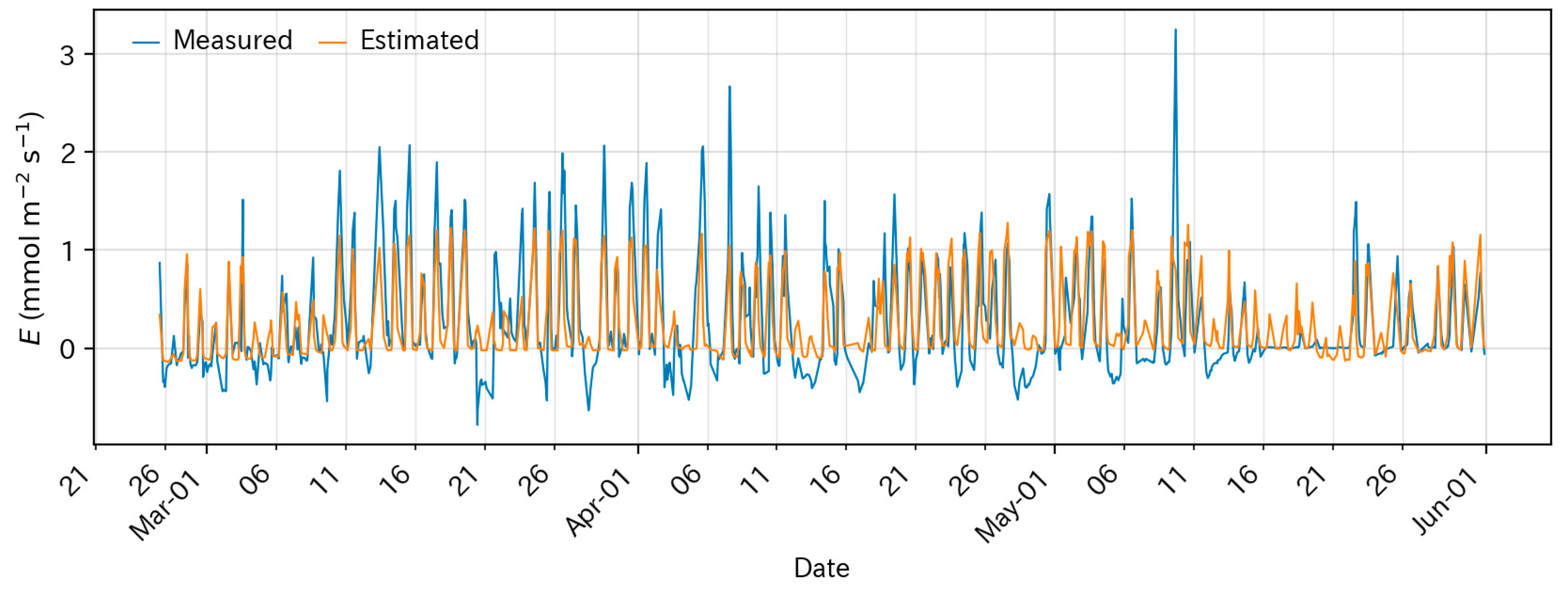
2.2.3. Fertigation Based on Estimated Evapotranspiration (ET)

In the ET-based treatment, I was determined based on the estimated hourly canopy evapotranspiration (E_h, L m⁻²), the main consumption element of irrigation water. E_h was calculated from the time integral of the instantaneous canopy evapotranspiration rate (E) estimated using a neural network model [36,37]. This neural network model accepts two input variables: the leaf transpiration rate (E_L) and leaf area index (LAI). E_L was estimated in the same manner as that reported by [36]. from above-ground environmental variables, such as Q, C_a, T_a, and RH, using a combination of a biochemical leaf photosynthesis model [38], semiempirical stomatal conductance model [39], one-dimensional heat and mass transfer model [40], and energy budget in the leaf [41,42]. LAI was estimated from nadir photographs using the method of [43]; an internet protocol (IP) camera (BB-SW175A, Panasonic Holdings Corporation, Osaka, Japan) was installed above each of the three experimental plots in the ET-based treatment, and nadir photographs were taken and sent to the laptop every hour. Then, LAI was estimated from the gap fraction (i.e., the fraction of non-leaf area) by applying the Beer–Lambert law [43]. The preparation of a pretrained neural network model is explained in Appendix A.1. From the calculated E_h, I (in L plot⁻¹) was calculated by the following equation:

$$I=f_{\mathrm{s}}LW{E}_{\mathrm{h}},$$

(1)

where L and W are the length (3 m) and effective width (i.e., the mean width of the top and bottom of the ridge, 1.35 m), respectively, and f_s is the factor of safety. We empirically set the value of f_s as 1.2 to consider many uncertainties, such as the loss of irrigation water due to vertical and horizontal percolations, evaporation from the soil surface, and the evapotranspiration model error.

2.2.4. Fertigation Based on Soil Moisture (SM)

In the SM-based treatment, the nutrient solution was supplied to maintain a constant θ within the ridge. When θ became less than a predetermined θ (θ_th), I (in L plot⁻¹) was calculated by the following equation:

$$I={\displaystyle \frac{LWD\left({\mathsf{\theta }}_{\mathrm{t}\mathrm{h}}-\mathsf{\theta }\right)}{{10}^3}},$$

(2)

where D is the depth (0.3 m) of the experimental plots. θ_th was set as 0.35 (cm³ cm⁻³), which corresponded to pF 1.16 (see Section 2.4).

Notably, in the SM-based treatment, I was calculated for each of the three replicated experimental plots based on θ measured by the corresponding soil moisture sensor. Similarly, in the ET-based treatment, I was calculated for each experimental plot based on the LAI estimated by the corresponding IP camera. In the AR-based treatment, in contrast, I was calculated based on Q measured by a single quantum sensor in the greenhouse and thus was the same among the three replicated experimental plots.

2.3. Measurement of Leaf Photosynthetic Parameters

At the end of the cultivation period (i.e., 17 and 19 April 2023), leaf photosynthetic parameters were estimated for the AR-, ET-, and SM-based treatments to determine whether these different fertigation treatments could affect the photosynthetic performance of Chinese chive.

The maximal carboxylation rate ($V_{\mathrm{c}\mathrm{m}\mathrm{a}\mathrm{x}}$) and maximal electron transport rate ($J_{\mathrm{m}\mathrm{a}\mathrm{x}}$) in the biochemical photosynthesis model of [38]) were estimated from the measured relationship between the leaf photosynthetic rate (A_L) and intercellular CO₂ concentration rate (C_i) (i.e., A_L-C_i curves). These leaf-scale measurements were performed using three portable photosynthesis systems (LI-6800, LI-COR Biosciences Inc., Lincoln, NE, USA). With the 2 cm² leaf chambers of the LI-6800 photosynthesis systems (6800-01A), leaves (approximately 50 mm away from the leaf tips) were clamped and acclimated to PPFD incident on the leaves (Q_L) of 1200 µmol m⁻² s⁻¹ for 8 min. Then, the values of A_L and C_i were recorded at chamber CO₂ concentrations (C_{a, cham}) of 400, 250, 100, 50, 400, 550, 700, 900, 1200, 1500, and 1800 µmol mol⁻¹ at 1.5 min intervals [44]. This procedure was performed at a constant leaf temperature (T_L) and then repeated at three different T_L values of 25, 30, and 35 °C. The relative humidity inside the leaf chamber (RH_cham) was kept as high as possible (ca. 55%) so as not to cause any leaf water stress. Four fully expanded young leaves in each of the AR-, ET-, and SM-based treatments were analyzed for each T_L; in total, 36 leaves were analyzed (i.e., 4 leaves × 3 T_L values × 3 treatments). To cancel instrumental errors associated with the three different portable photosynthesis systems, these systems were rotated among the three treatments (i.e., after the completion of an A-C_i curve, the portable photosynthesis system was moved to another treatment). Since the width of Chinese chive leaves was narrower than the diameter of the 2 cm² leaf chamber, the leaf width was measured and used for correcting the autocalculated A_L. The measured A_L-C_i relationships were fit by the equations of the photosynthesis model (see Appendix A.2) to estimate the unknown parameters V_cmax and J_max. After visual inspection of the A_L-C_i curves, the region with C_i < 400 was assumed to be limited by V_cmax, and the region with 400 ≤ C_i was assumed to be limited by J_max. Each of the two sections in the A_L-C_i curves was fit with the corresponding equation based on the Levenberg–Marquardt method using the Python “lmfit” package (version 1.0.1; [45]). For V_cmax-limited photosynthesis, two parameters, namely, V_cmax and the day respiration (R_d), were estimated by fitting Equation (A2). For J_max-limited photosynthesis, the electron transport rate (J) was estimated by fitting Equation (A3) and then used to invert J_max from Equations (A4) and (A5). In the curve-fitting processes for J_max-limited photosynthesis, the R_d value estimated in the V_cmax-limited curve fitting was used as a fixed parameter [44]. The values of the other model parameters were obtained from the literature [46,47].

In addition to V_cmax and J_max, the slope (g₁) and intercept (g₀) of the semiempirical stomatal conductance model of [39] (often called the unified stomatal optimization (USO) model) were estimated from the measurements of $A_{\mathrm{L}}$ against Q_L. After the leaves were clamped in a 2 cm² leaf chamber and acclimated at Q_L = 900 µmol m⁻² s⁻¹ for 10 min, the values of Q_L were changed stepwise to 1500, 1200, 600, 300, 150, 75, and 0 µmol m⁻² s⁻¹ at ten min intervals. During the measurements, C_a, T_L, and RH were set at 400 µmol mol⁻¹, 25 °C, and ca. 60%, respectively. Four fully expanded leaves were analyzed for each treatment. The relationship between the stomatal conductance to water vapor (g_sw) and the combined environmental–physiological index (${\displaystyle \frac{1.6A_{\mathrm{L}}}{C_{\mathrm{s}}\surd D}}$) was linearly regressed to obtain g₀ and g₁ using the Python statsmodels library (version 0.13.5, [48]).

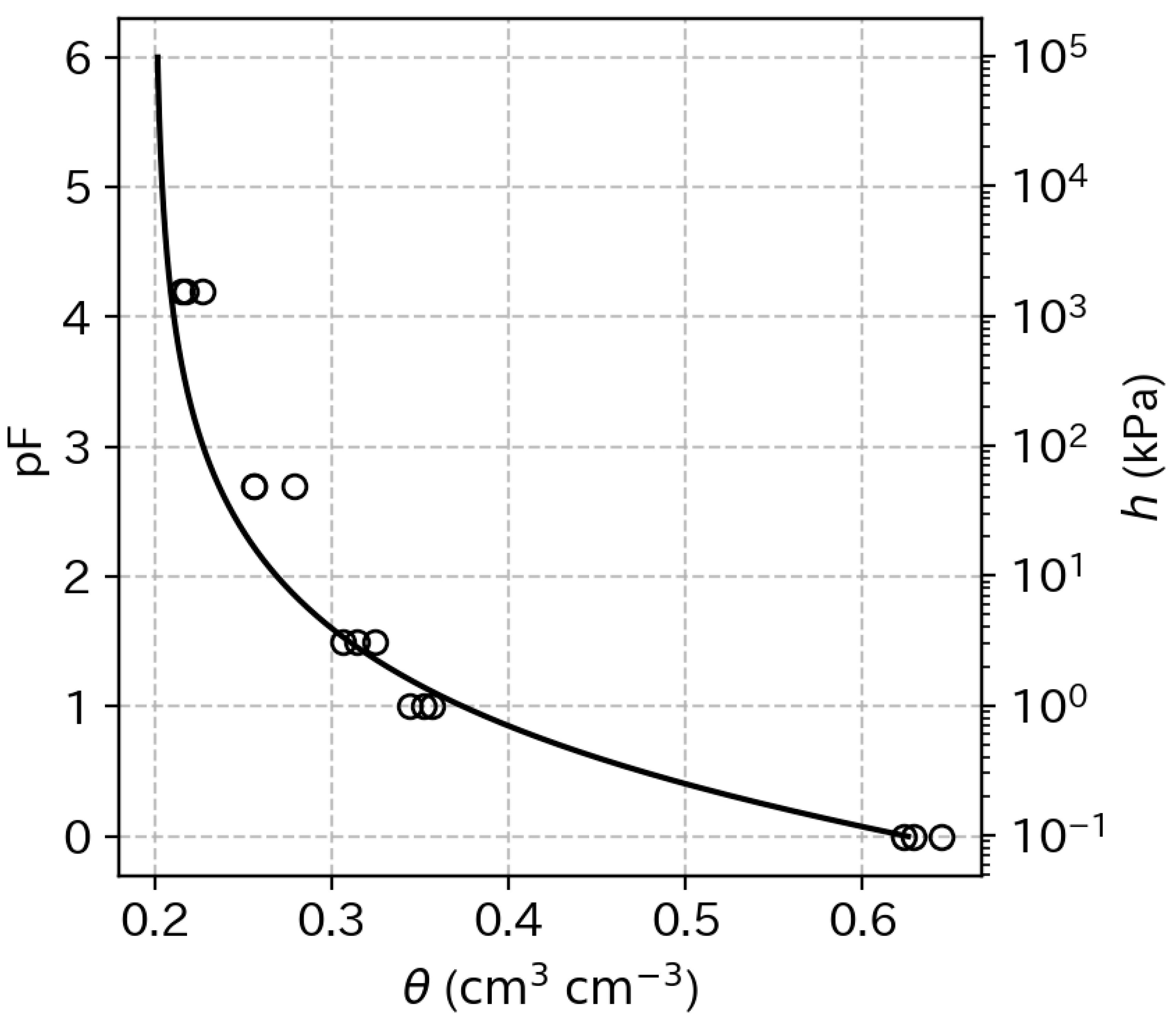
2.4. Measurement of Soil Water Retention Characteristics

Soil water availability is often expressed as the suction head (h; cm) and pF (i.e., log₁₀h). To convert the measured θ to h and pF, the relationship between θ and h (and pF; soil water retention curve) was determined in the laboratory. Three 100 mL soil cores were sampled from the control treatment at a depth of 15 cm on 6 March 2023, and saturated with water for two days. Then, the saturated soil samples were equilibrated at suction heads of 10 and 31.6 cm (i.e., pF 1.0 and 1.5) at two-day intervals using a suction table (DIK-3520, Daiki Rika Kogyo Co, Ltd., Saitama, Japan). After the pF 1.5 measurement, the soil cores were placed on a porous suction plate for further dehydration for two days, and the remaining water contents were regarded as θ at a suction head of 500 cm (i.e., pF 2.7; [49]. Then, the soil cores were further dehydrated using a centrifuge (SS-2050A, Sakuma Seisakusho, Tokyo, Japan) at a suction head of 15,800 cm (i.e., pF 4.2). These measured θ-h relationships were fit with the following van Genuchten equation for interpolation [50]:

$$\mathsf{\theta }={\mathsf{\theta }}_{\mathrm{r}}+{\displaystyle \frac{{\mathsf{\theta }}_{\mathrm{s}}-{\mathsf{\theta }}_{\mathrm{r}}}{{\left(1+{\left(\alpha h\right)}^n\right)}^{1-1/n}}}$$

(3)

where θ_r is the residual volumetric water content (dimensionless), θ_s is the saturated volumetric water content (dimensionless), α is a parameter corresponding approximately to the inverse of the air-entry value (cm⁻¹), and n is a shape parameter. Figure 2 shows the obtained soil water retention curve. According to this curve, θ_th = 0.35, at which fertigation is triggered in the SM-based treatment, corresponded with pF 1.16.

2.5. Statistical Analysis

The effects of different fertigation treatments on the yields and photosynthetic parameters of Chinese chive were statistically evaluated. For FW, V_cmax, and J_max, an overall difference among the four treatments was determined by one-way analysis of variance (ANOVA). Additionally, pairwise comparisons between individual treatments were made by Tukey’s honest significant difference (HSD) test. These statistical analyses were performed using scipy (1.7.3), statsmodels (0.13.5), and pingouin (0.5.1), free software libraries available in Python (3.10.12) (the numbers in parentheses indicate the software versions). To evaluate the effect of different fertigation treatments on stomatal responses, the three regression lines (corresponding to the SM-, ET-, and AR-based treatments) between g_sw and ${\displaystyle \frac{1.6A_{\mathrm{L}}}{C_{\mathrm{s}}\surd D}}$ were compared using analysis of covariance (ANCOVA) using R (4.0.2; R Core Team, 2017). For post hoc pairwise comparisons of these slopes obtained from the regression analysis, the emtrends function from the emmeans package (1.10.3) in R was employed [51]. This function allowed for the estimation and comparison of trends (slopes) among the treatments. To account for multiple comparisons, the Bonferroni correction method was applied.

3. Results

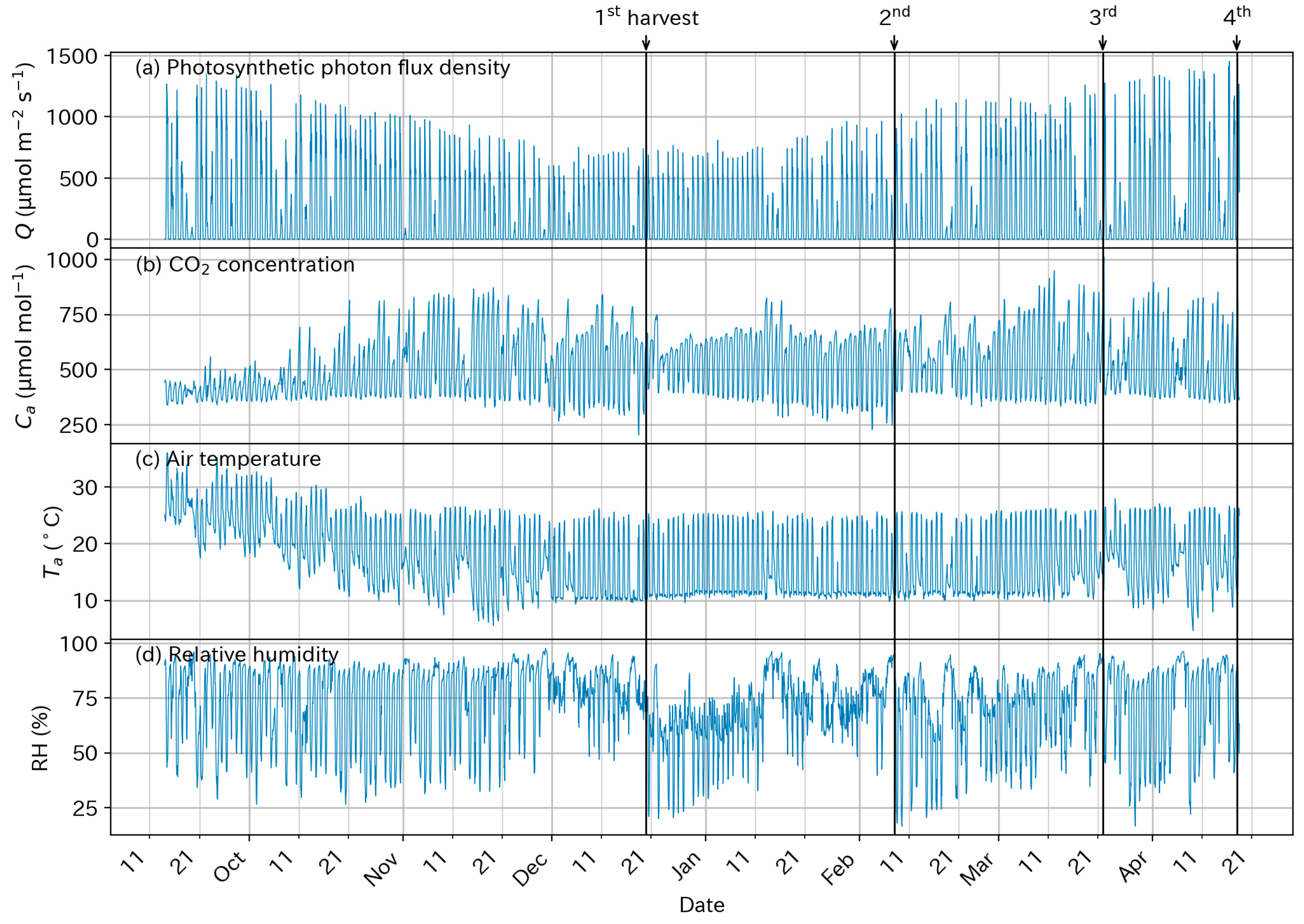
3.1. Above-Ground Environmental Conditions

Figure 3 shows time-course changes in the above-ground environmental elements. All variables showed seasonal changes typical of a greenhouse in Japan. In (a), Q values reached approximately 1300 μmol m⁻² s⁻¹ on sunny days in October and then gradually decreased until the winter solstice on 22 December, around which Q barely reached 750 μmol m⁻² s⁻¹. Then, Q started to increase until the end of the experiment in April. In (b), C_a showed a diurnal change due to the photosynthesis and respiration of the Chinese chive canopy in the greenhouse; C_a decreased to as low as 300 μmol mol⁻¹ during daytime hours due to the photosynthesis of the Chinese chive canopy and increased to 800 μmol mol⁻¹ due to canopy respiration at night. The magnitude of the diurnal change in C_a was small when the leaf area of the Chinese chive canopy was small (i.e., immediately after transplantation or harvest) but gradually became larger toward the next harvest as the canopy leaves grew. These results indicate that the amount of the leaf area in the greenhouse influenced the canopy-scale carbon exchange [52]. In (c), T_a was greatly affected by environmental control in the greenhouse; thanks to the automatic control of the top and side greenhouse windows, daytime T_a values could be maintained at less than 26 °C for most of the time, except for the first two months (i.e., September and October), in which the temperature outside the greenhouse was very high. Additionally, from December 1, on which the automatic control of the nighttime heater was turned on, T_a was maintained above 10 °C. In (d), RH increased at night up to 95% due to the closure of the greenhouse windows and a decrease in T_a. During the daytime, in contrast, RH decreased to as low as 25% due to the ventilation of the greenhouse and an increase in T_a. Immediately after the first and second harvests, the daytime RH values were lower than those before the harvest and gradually increased until the next harvest. These results suggest that similar to C_a, the humidity inside the greenhouse depended on the amount of the transpiring leaf area.

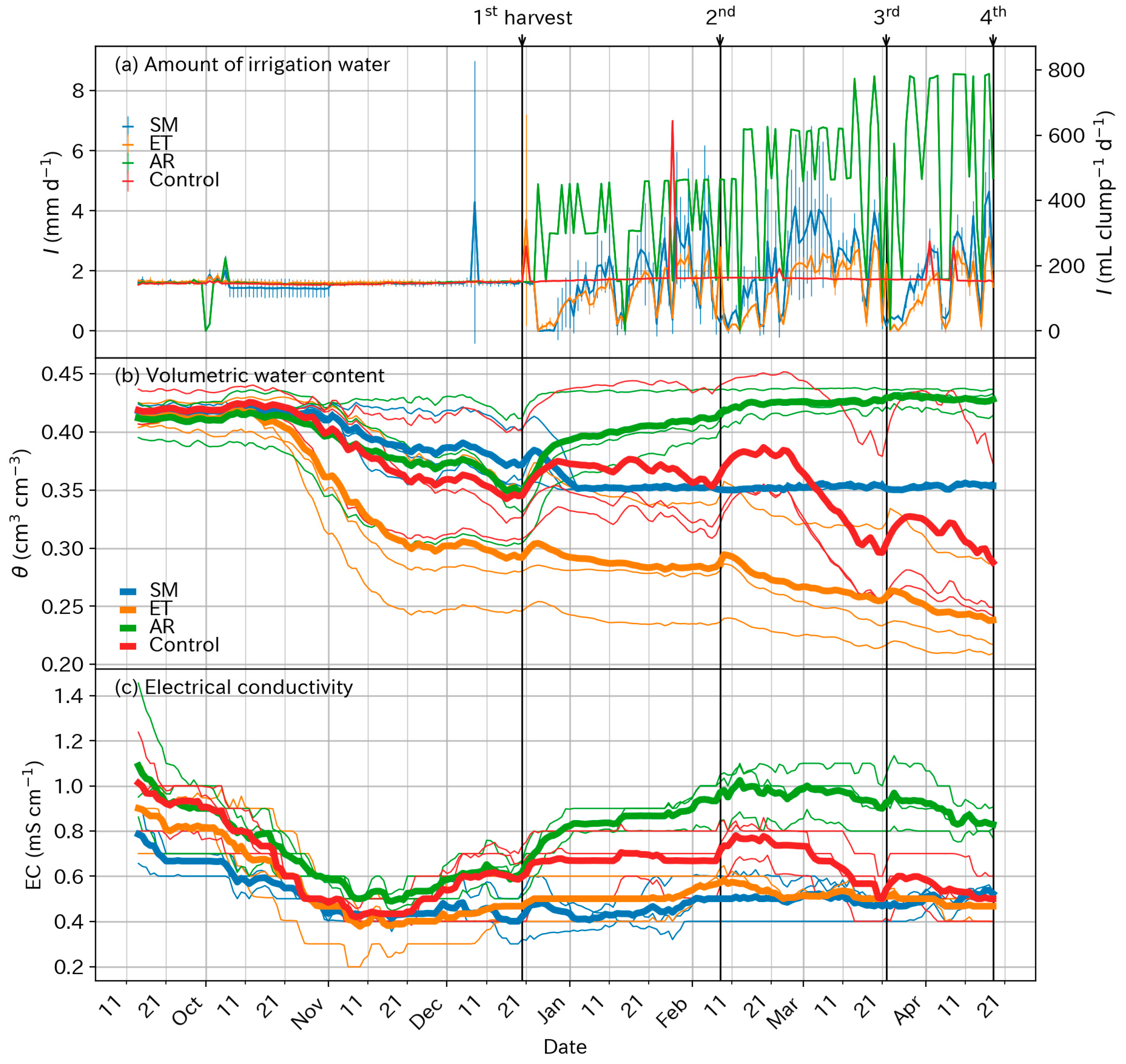
3.2. Supplied Water and Soil Conditions

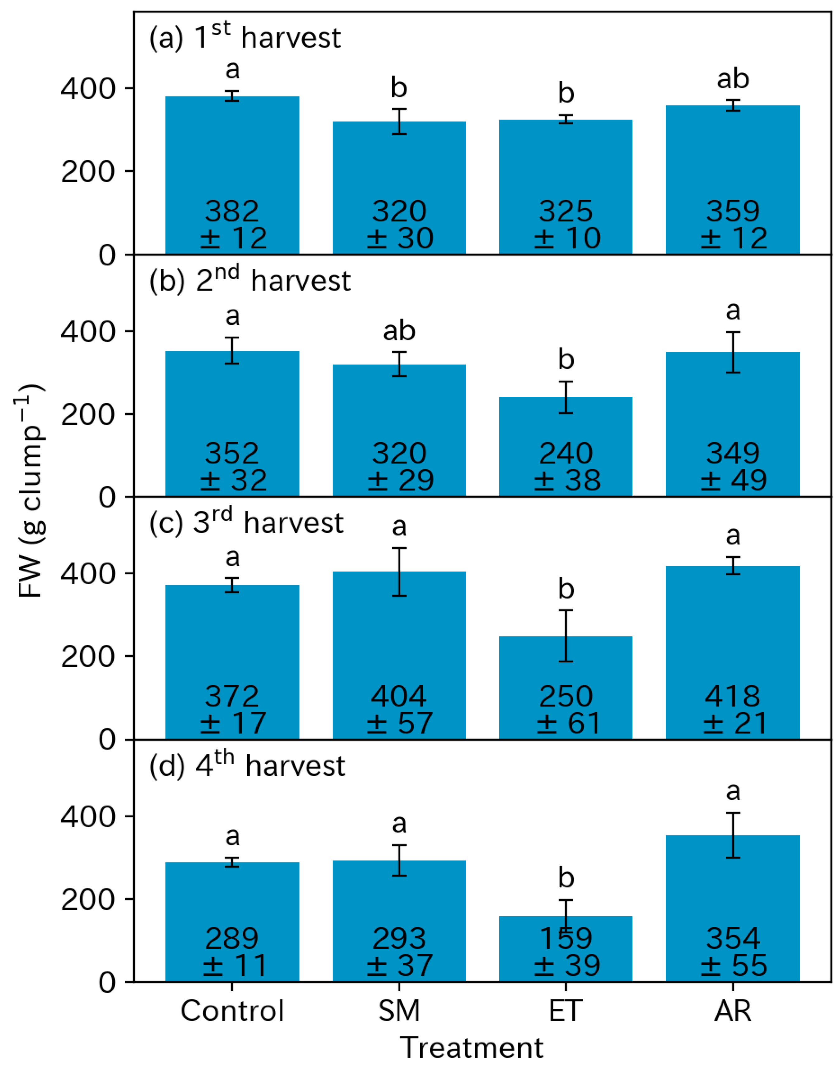
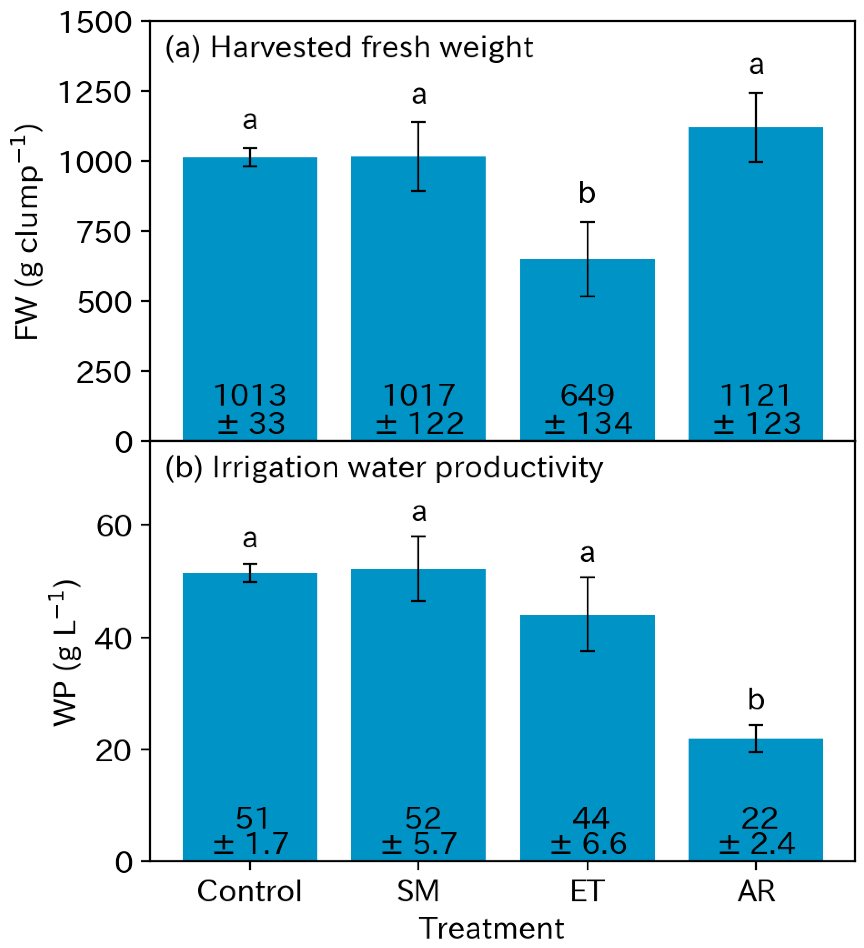
Figure 4 shows daily changes in I, θ, and EC in the soil. From transplantation to the first harvest (20 December 2022), all experimental plots were supplied with the same daily I (150 mL clump⁻¹ d⁻¹). Then, after the first harvest, the daily I varied as the four different fertigation treatments began.

The AR-based treatment, in which I was determined based on Q in the greenhouse, supplied the highest I among the four fertigation treatments. From the first harvest until the middle of February, the daily I in the AR-based treatment was either 150, 300, or 450 mL clump⁻¹, depending on the weather conditions. Then, as Q increased (see Figure 3a), daily I reached 600 mL clump⁻¹ d⁻¹ and even 750 mL clump⁻¹ d⁻¹ in March and April. As a result of this abundant water supply, θ in the AR-based treatment began to increase from the beginning of the treatment; in all three experimental plots, the daily means of θ gradually increased and converged to approximately 43% at the end of the experiment in April.

In the SM-based treatment, θ was successfully maintained at approximately 35% (i.e., θ_th) after the first harvest. Daily I, in contrast, showed a cyclical change depending on the leaf area of the Chinese chive canopy; daily I became almost zero immediately after a harvest and gradually increased (i.e., many fertigation events were triggered within a day) toward the next harvest as the leaf area increased. These results strongly suggest that the leaf area of the Chinese chive canopy is a strong determinant of the canopy evapotranspiration and that crop water demand can vary dynamically with the leaf area.

In the ET-based treatment, in which I was determined based on the amount of estimated canopy evapotranspiration, the pattern of change in I was very similar to that in the SM-based treatment; daily I showed a cyclical change depending on the leaf area of the Chinese chive canopy. This observed similarity in the I of the SM and ET-based treatments adds validity to the estimation of the canopy evapotranspiration rate in the ET-based treatment. However, the ET-based treatment tended to supply a smaller daily I than the SM-based treatment. As a result, θ in the ET-based treatment gradually declined from the first harvest until the end of the experiment.

In the control treatment, where a constant daily I was supplied (150 mL clump⁻¹ d⁻¹), θ increased for several days after a harvest and then gradually declined until the next harvest. This pattern of change in θ can be explained by the pattern of leaf growth; when the leaf area was small (i.e., after a harvest), the constant daily I was in excess of the water demand of the Chinese chive canopy, causing an increase in θ. However, as the leaves grew, the water demand of the Chinese chive canopy exceeded the constant I, causing a decline in the soil water. Again, these results indicate the importance of considering the canopy leaf area for optimizing the irrigation water supply.

In Figure 4c, at the time of transplantation, EC in the 12 experimental plots showed substantial variations, ranging between 0.6 and 1.4 mS cm⁻¹. Then, EC gradually decreased to ca. 0.4 mS cm⁻¹ until mid-November, when the liquid fertilizer supply started. Since then, the EC in the four treatments started to diverge. The EC in the AR-based treatment was the highest among the four treatments because abundant fertilizer was supplied with the irrigation water. However, EC in the other three treatments did not change in tandem with I. For example, EC in the SM-based treatment was lower than that in the ET-based treatment, despite the higher I in the SM-based treatment than in the ET-based treatment.

3.3. Yields

Figure 5 shows the FW of the harvested Chinese chive plants under the four different fertigation treatments. After the first harvest, when the four different fertigation treatments were started, the FW of the ET-based treatment was always the lowest among the four treatments (Figure 5b–d); at the second, third, and fourth harvests, the mean FW of the ET-based treatment corresponded to only 68, 67, and 55%, respectively, of the control treatment. These results were most likely caused by the lowest I in the ET-based treatment; the ET-based treatment’s total I between two harvests (i.e., first to second, second to third, and third to fourth) was only 70, 84, and 69%, respectively, of that of the control treatment (see Figure 4a). As a result of such low I in the ET-based treatment, θ declined gradually, suppressing the growth of the Chinese chive. No significant difference was detected between any pairs of the other three treatments (i.e., control, SM, and AR), although the AR-based treatment with the highest water supply had the highest FW at the third and fourth harvests; for example, at the fourth harvest, the FW in the AR-based treatment was 122% of that in the control treatment. These results suggest that under the current experimental setting, maintaining a very high θ value may positively influence the growth of Chinese chive.

Figure 6 further exemplifies the importance of θ for FW. In Figure 6, there was a highly significant, proportional relationship between time-average θ ($\overline{\mathsf{\theta }}$) and FW (correlation coefficient r = 0.65). A decline in FW was especially apparent when $\overline{\mathsf{\theta }}$ became lower than 0.3. Above $\overline{\mathsf{\theta }}$ = 0.3, the relationship between $\overline{\mathsf{\theta }}$ and FW was less apparent, although at the fourth harvest, the FW of $\overline{\mathsf{\theta }}$ > 0.4 appeared to be higher than that of $\overline{\mathsf{\theta }}$ ≂ 0.35. In Figure 7, the horizontal axis $\overline{\mathsf{\theta }}$ of Figure 6 was converted to time-average pF ($\overline{\mathrm{p}\mathrm{F}}$) using the soil water retention curve (Figure 2). Similar to the $\overline{\mathsf{\theta }}$–FW relationship, there was a highly significant relationship between $\overline{\mathrm{p}\mathrm{F}}$ and FW (r = −0.72).

Note that at the first harvest in Figure 5a (i.e., before the four different fertigation treatments started), ANOVA detected a significant difference among the mean FWs in the four treatments, even though all experimental plots were supplied with a constant I until the first harvest. Tukey’s HSD test also indicated that the FW of the control treatment was significantly higher than that of the SM- and ET-based treatments. These results may have been caused by several factors, such as the nonuniformity of initial soil conditions and Chinese chive seedlings.

3.4. Water Productivity

As a result of the different fertigation treatments, the corresponding WP (i.e., FW divided by ΣI; [1]) differed significantly (Figure 8). The AR-based treatment had the lowest WP, despite the highest harvested FW, due to the apparent over-fertigation. The WP of the ET-based treatment was higher than that of the AR-based treatment but much lower than that of the SM-based and control treatments due to the lowest harvested FW.

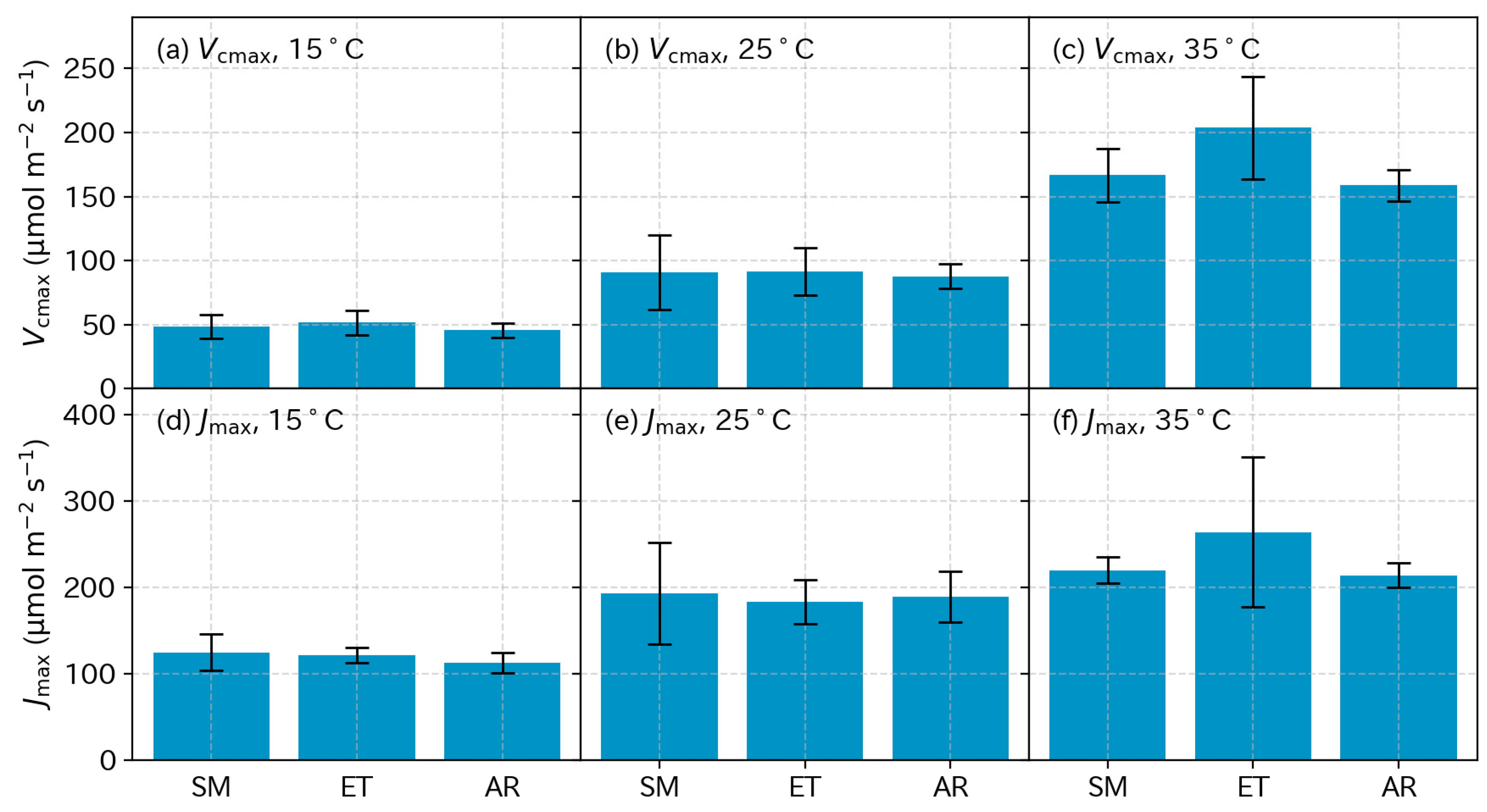
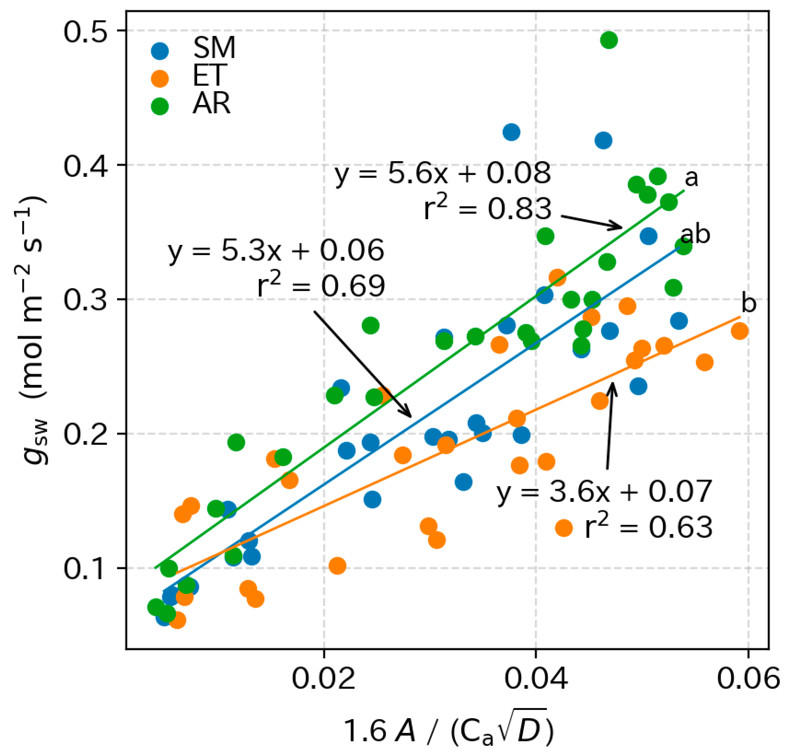
3.5. Photosynthetic Parameters

Figure 9 shows the leaf photosynthetic capacity (V_cmax and J_max) estimated for the SM-, ET-, and AR-based treatments. Since V_cmax and J_max were estimated at the end of the experiment (i.e., 17 and 19 April 2023), the estimated values should reflect the influence of the three different fertigation treatments and resultant θ (see Figure 4). Despite the large difference in θ, the three fertigation treatments did not seem to affect V_cmax and J_max much; no clear relationship was found between θ and V_cmax or J_max (an exception was J_max at 35 °C in the ET-based treatment, in which an apparent outlier raised the mean value). ANOVA did not detect significant differences in either V_cmax or J_max at any of the three T_L values. These results suggest that the influence of I and θ on Chinese chive’s leaf photosynthetic capacity was only marginal.

Figure 10 shows the relationship between g_sw and the combined environmental-physiological index (${\displaystyle \frac{1.6A_{\mathrm{L}}}{C_{\mathrm{s}}\surd D}}$) of the USO model [39]. All three regression lines corresponding to the SM-, ET-, and AR-based treatments had high values of the coefficient of determination (r²) (i.e., r² ≧ 0.63), indicating the applicability of the USO model to Chinese chive leaves. The regression lines for the AR- and SM-based treatments were similar (i.e., y = 5.6 x + 0.08 and y = 5.3 x + 0.06, respectively), whereas that of the ET-based treatment had a substantially smaller slope parameter (i.e., y = 3.6 x + 0.07). The smaller slope of the ET-based treatment was probably caused by water stress imposed by the lower I and θ. ANCOVA revealed a significant interaction between ${\displaystyle \frac{1.6A_{\mathrm{L}}}{C_{\mathrm{s}}\surd D}}$ and the treatments (p = 0.03). A significant difference was observed between the slopes of the AR- and SM-based treatments (p = 0.03), indicating that the different fertigation treatments affected the slopes of the stomatal conductance model.

4. Discussion

4.1. Advantages and Disadvantages of the Different Fertigation Methods

This study applied four different fertigation scheduling methods to cultivate Chinese chive. The results clearly illustrated some advantages and disadvantages of the different fertigation methods.

The ET-based treatment supplied the lowest I (Figure 4a), resulting in the lowest yield (Figure 5). I in the ET-based treatment was calculated by a neural network model, which was calibrated and validated based on E measured by the open chamber method. Although the trained neural network model could reproduce the measured E with reasonable accuracy (Figure A1 in Appendix A.1), it is possible that the chamber-measured E underestimated the actual E in the greenhouse (i.e., without a chamber); it has been pointed out that installing a chamber over a crop canopy affects the microclimate around the crop canopy [53,54]. The placement of the open chamber possibly reduced E due to, e.g., reduced leaf boundary layer conductance caused by restricted airflow and reduced stomatal conductance caused by increased temperature in the chamber [55]. To compensate for any uncertainties of the I estimation, the model-estimated E was multiplied by a safety factor of 1.2 (see Equation (1)). However, the final I still seemed to be insufficient, as θ was gradually depleted throughout the cultivation period in the ET-based treatment (Figure 4b). These results illustrate the risk of prediction-based fertigation methods, as errors in E prediction can accumulate over time [11].

In contrast to the ET-based treatment, I in the AR-based treatment seemed to overestimate water consumption in the Chinese chive canopy, causing a gradual increase in θ (Figure 4b). The daily average θ saturated at approximately 0.43 toward the end of the cultivation period. The over-fertigation in the AR-based treatment should have been alleviated by setting a higher Q_th value at which fertigation was triggered, as Q_th in this study was determined based on the maximum transpiration rate reported in a previous study [33] (see Section 2.2.2). The over-fertigation, however, did not cause any yield loss in Chinese chive (Figure 5), which could have occurred due to insufficient aeration [56,57]. The lack of any yield loss may be attributed to the ridge–furrow cultivation system, which drained excess moisture from the ridges to the furrows (Figure 1b) [58,59]. Additionally, sufficient temporal and spatial fertigation intervals should have contributed to adequate aeration in the soil (i.e., in the AR-based treatment, fertigation events were triggered at several-hour intervals from 20 cm apart drippers on three parallel driplines). According to the sampled soil core data, the maximum θ is approximately 0.63 (Figure 2), and thus, the volumetric air content (i.e., air-filled porosity) in the AR-based treatment was maintained, at least, at 20% (i.e., 0.63 minus 0.43). These results indicate that over-fertigation is unlikely to be a severe problem when cultivating Chinese chive in a drip-fertigated, ridge–furrow system, although this conclusion probably depends on soil texture [60].

In the SM-based treatment, θ was successfully maintained at θ_th (=0.35; Figure 4b). The SM-based treatment required much less I than the AR-based treatment while achieving comparable FW to that of the AR-based treatment. These results illustrate the advantage of “feedback” control, in which measured θ was used to adjust I. Since θ is one of the most influential variables for crop yield (see Figure 6), the θ-based control of I in the SM-based treatment seems reasonable. It should be noted, however, that the SM-based method can fail to improve crop yields, as [61] reported for apple trees; the success of the SM-based method depends on many factors, such as the accuracy and reliability of soil moisture measurements, the depth of soil moisture installation, and an appropriate θ_th value at which fertigation is triggered [62].

The fertigation pattern in the ET-based treatment was very similar to that in the SM-based treatment (Figure 4a), although the total I in the ET-based treatment was 27% less than that in the SM-based treatment. These results indicate that the ET-based method using the neural network model could have supplied irrigation water as desirably as the SM-based method if the estimated E_h had been multiplied by a higher safety factor (see Equation (1)). Using other, more frequently used evapotranspiration models (e.g., FAO Penman–Monteith model) [63] may have yielded better results, although these models would have required parameter optimizations for application to Chinese chive. Nevertheless, the similarity of the fertigation patterns in the ET- and SM-based methods suggests that the ET-based method (i.e., fertigation scheduling based on the greenhouse weather and crop growth stage) is a plausible option once appropriate model parameterization is performed. In contrast, I in the AR-based treatment inevitably deviated from that in the SM-based treatment, as the AR-based treatment did not consider the change in LAI.

One limitation of our study is that the amount of fertilizer supplied was proportional to the irrigated water. This approach was deliberately chosen to simulate realistic agricultural practices, where irrigation and fertilization are often linked to maximize efficiency and reduce labor. While this method mirrors actual field conditions, it introduces potential confounding effects, as variations in crop growth could be attributed to differences in both irrigation and fertilization. Future studies might consider separating these variables by applying a consistent fertilizer amount across treatments, regardless of the irrigation volume. However, it is important to recognize that such an approach has its own drawbacks. By isolating irrigation from fertilization, studies may create scenarios that are less representative of practical farming operations. Consequently, the findings from such studies may have limited applicability in real-world agricultural settings. Our study aims to balance realism and experimental control, providing insights that are directly applicable to typical agricultural practices, even if this comes at the expense of some experimental precision.

4.2. Optimum Moisture for Chinese Chive Cultivation

An optimum θ value for maximizing crop yields depends on crop species and many other site-specific factors (e.g., soil texture, evaporative demand, or root distribution) and thus is not well defined. Traditionally, maintaining θ near the field capacity (i.e., pF 2.0 to 2.5) is regarded as a good irrigation practice [62,64]. For example, for greenhouse-grown vegetable crops with high-frequency irrigation, soil matric potential intervals of −10 to −20 kPa (pF 2.0 to 2.3), −10 to −30 kPa (pF 2.0 to 2.5), and −20 to 40 kPa (pF 2.3 to 2.6) for coarse-, medium-, and fine-textured soils, respectively, have been suggested [65]. Other authors suggested even lower soil moisture values [66]. In our experiment, the yield of Chinese chive increased above those typical field capacity ranges (Figure 7). These results suggest the possibility of further improving crop yields by maintaining higher θ than the typical field capacity range. However, it should be noted that the threshold value of θ for triggering irrigation also depends on the positioning of soil-moisture sensors relative to drip lines [67,68]. In many practical cases, θ is usually measured at a point, and its representativeness over an entire root zone depends on many factors such as the positioning of driplines, the spatial distribution of the soil hydraulic conductance, and the existence of a plow pan. In this research, we determined the positions of the soil-moisture sensors empirically (see Figure 1), but their appropriateness should be evaluated based on numerical simulation in future research [67]. Additionally, for Chinese chive, an optimal θ range may depend on the growth stage; for example, Chinese chive shoots start to tiller (i.e., produce lateral shoots) using carbohydrates stored in the belowground organs (roots and bulbs) after leaves grow to a certain point [29]. This tillering stage may be more prone to water stress than other stages. Optimum fertigation scheduling may need to consider these growth stage-dependent factors.

4.3. Photosynthetic Parameters

Different fertigation treatments caused a significant difference in the slope parameter g₁ in the USO model; the ET-based treatment under water stress had a smaller slope parameter than the well-watered AR- and SM-based treatments (Figure 10). This response is in accordance with previous research [69,70]. For example, Héroult et al. (2013) reported that two humid tree species (E. dunnii and E. saligna) showed reductions in g₁ of 75% and 39% under drought [69]. In our experiment, g₁ in the water-stressed ET-based treatment was 35% less than that in the well-watered AR-based treatment. This decline in g₁ (and, consequently, g_sw) in the ET-based treatment could be one of the reasons for reduced harvested FW; reduced g_sw should have caused a reduction in photosynthesis, resulting in reduced crop growth.

In contrast to the slope parameter in the USO model, no significant difference was found in the photosynthetic capacity (V_cmax and J_max) among the AR, SM, and ET-based treatments. These results are consistent with the findings from some prior studies but not others; several studies reported a decline in V_cmax and J_max due to drought conditions [20,21,22], whereas other studies reported that V_cmax and J_max changed only marginally under drought [23,24]. Galmés et al. [19] demonstrated that stomatal closure was the typical limitation of photosynthesis in response to mild water stress and that V_cmax and J_max could limit photosynthesis only under severe water stress. In our study, Chinese chive leaves in the ET-based treatment were exposed to moderate water stress (i.e., $\overline{\mathrm{p}\mathrm{F}}=3.8$). This water stress was possibly not severe enough to cause a decline in V_cmax and J_max.

5. Conclusions

This study evaluated the effects of four different fertigation scheduling methods on Chinese chive cultivation, focusing on crop yields and leaf photosynthetic parameters. The different methods caused significant variations in I and θ, which impacted crop yields differently.

The ET-based method supplied inadequate I, leading to a severe yield loss. This method was susceptible to accumulated errors in estimated E and caused a gradual depletion of θ due to the lack of feedback control based on θ. In contrast, the AR-based method provided excess water, resulting in low WP. This method could lead to over-/under-fertigation without frequent adjustments of Q_th because the water demand of a Chinese chive crop canopy can change drastically with LAI.

The SM-based method successfully maintained the target soil moisture level and achieved the highest WP. It presented a lower risk of under-/over-fertigation, as I was controlled based on measured θ. Although determining the optimal θ_th is necessary, this method appears suitable for small-scale greenhouse cultivation where soil nonuniformity is minimal.

Ridge-cultivated Chinese chive showed resilience to over-fertigation, as no yield loss was observed in the overirrigated AR-based treatment. Additionally, different fertigation methods did not affect leaf photosynthetic capacity (V_cmax and J_max), whereas inadequate fertigation significantly reduced g_sw.

References

1. Fernández, J.E.; Alcon, F.; Diaz-Espejo, A.; Hernandez-Santana, V.; Cuevas, M.V. Water Use Indicators and Economic Analysis for On-Farm Irrigation Decision: A Case Study of a Super High Density Olive Tree Orchard. Agric. Water Manag. 2020, 237, 106074. [Google Scholar] [CrossRef]
2. Li, H.; Mei, X.; Wang, J.; Huang, F.; Hao, W.; Li, B. Drip Fertigation Significantly Increased Crop Yield, Water Productivity and Nitrogen Use Efficiency with Respect to Traditional Irrigation and Fertilization Practices: A Meta-Analysis in China. Agric. Water Manag. 2021, 244, 106534. [Google Scholar] [CrossRef]
3. Sinha, I.; Buttar, G.S.; Brar, A.S. Drip Irrigation and Fertigation Improve Economics, Water and Energy Productivity of Spring Sunflower (Helianthus annuus L.) in Indian Punjab. Agric. Water Manag. 2017, 185, 58–64. [Google Scholar] [CrossRef]
4. Xiukang, W.; Yingying, X. Evaluation of the Effect of Irrigation and Fertilization by Drip Fertigation on Tomato Yield and Water Use Efficiency in Greenhouse. Int. J. Agron. 2016, 2016, 3961903. [Google Scholar] [CrossRef]
5. Azad, N.; Behmanesh, J.; Rezaverdinejad, V.; Abbasi, F.; Navabian, M. An Analysis of Optimal Fertigation Implications in Different Soils on Reducing Environmental Impacts of Agricultural Nitrate Leaching. Sci. Rep. 2020, 10, 7797. [Google Scholar] [CrossRef] [PubMed]
6. Zhang, T.Q.; Tan, C.S.; Liu, K.; Drury, C.F.; Papadopoulos, A.P.; Warner, J. Yield and Economic Assessments of Fertilizer Nitrogen and Phosphorus for Processing Tomato with Drip Fertigation. Agron. J. 2010, 102, 774–780. [Google Scholar] [CrossRef]
7. Incrocci, L.; Thompson, R.B.; Fernandez-Fernandez, M.D.; De Pascale, S.; Pardossi, A.; Stanghellini, C.; Rouphael, Y.; Gallardo, M. Irrigation Management of European Greenhouse Vegetable Crops. Agric. Water Manag. 2020, 242, 106393. [Google Scholar] [CrossRef]
8. García, L.; Parra, L.; Jimenez, J.M.; Lloret, J.; Lorenz, P. IoT-Based Smart Irrigation Systems: An Overview on the Recent Trends on Sensors and Iot Systems for Irrigation in Precision Agriculture. Sensors 2020, 20, 1042. [Google Scholar] [CrossRef] [PubMed]
9. Nikolaou, G.; Neocleous, D.; Katsoulas, N.; Kittas, C. Irrigation of Greenhouse Crops. Horticulturae 2019, 5, 7. [Google Scholar] [CrossRef]
10. Gu, Z.; Qi, Z.; Burghate, R.; Yuan, S.; Jiao, X.; Xu, J. Irrigation Scheduling Approaches and Applications: A Review. J. Irrig. Drain. Eng. 2020, 146, 04020007. [Google Scholar] [CrossRef]
11. Jones, H.G. Irrigation Scheduling: Advantages and Pitfalls of Plant-Based Methods. J. Exp. Bot. 2004, 55, 2427–2436. [Google Scholar] [CrossRef]
12. Lemay, I.; Caron, J. Defining Irrigation Set Points Based on Substrate Properties for Variable Irrigation and Constant Matric Potential Devices in Greenhouse Tomato. HortScience 2012, 47, 1141–1152. [Google Scholar] [CrossRef]
13. Choi, K.Y.; Choi, E.Y.; Kim, I.S.; Lee, Y.B. Improving Water and Fertilizer Use Efficiency during the Production of Strawberry in Coir Substrate Hydroponics Using a FDR Sensor-Automated Irrigation System. Hortic. Environ. Biotechnol. 2016, 57, 431–439. [Google Scholar] [CrossRef]
14. Pereira, L.S.; Paredes, P.; Jovanovic, N. Soil Water Balance Models for Determining Crop Water and Irrigation Requirements and Irrigation Scheduling Focusing on the FAO56 Method and the Dual Kc Approach. Agric. Water Manag. 2020, 241, 106357. [Google Scholar] [CrossRef]
15. Morille, B.; Migeon, C.; Bournet, P.E. Is the Penman-Monteith Model Adapted to Predict Crop Transpiration under Greenhouse Conditions? Application to a New Guinea Impatiens Crop. Sci. Hortic. 2013, 152, 80–91. [Google Scholar] [CrossRef]
16. Vereecken, H.; Kasteel, R.; Vanderborght, J.; Harter, T. Upscaling Hydraulic Properties and Soil Water Flow Processes in Heterogeneous Soils: A Review. Vadose Zone J. 2007, 6, 1–28. [Google Scholar] [CrossRef]
17. Chaves, M.M. Effects of Water Deficits on Carbon Assimilation. J. Exp. Bot. 1991, 42, 1–16. [Google Scholar] [CrossRef]
18. Pinheiro, C.; Chaves, M.M. Photosynthesis and Drought: Can We Make Metabolic Connections from Available Data? J. Exp. Bot. 2011, 62, 869–882. [Google Scholar] [CrossRef] [PubMed]
19. Galmés, J.; Medrano, H.; Flexas, J. Photosynthetic Limitations in Response to Water Stress and Recovery in Mediterranean Plants with Different Growth Forms. New Phytol. 2007, 175, 81–93. [Google Scholar] [CrossRef]
20. Maroco, J.P.; Rodrigues, M.L.; Lopes, C.; Chaves, M.M. Limitations to Leaf Photosynthesis in Field-Grown Grapevine under Drought—Metabolic and Modelling Approaches. Funct. Plant Biol. 2002, 29, 451–459. [Google Scholar] [CrossRef]
21. Wei, Z.; Yanling, J.; Feng, L.; Guangsheng, Z. Responses of Photosynthetic Parameters of Quercus Mongolica to Soil Moisture Stresses. Acta Ecol. Sin. 2008, 28, 2504–2510. [Google Scholar] [CrossRef]
22. Albert, K.R.; Mikkelsen, T.N.; Michelsen, A.; Ro-Poulsen, H.; van der Linden, L. Interactive Effects of Drought, Elevated CO2 and Warming on Photosynthetic Capacity and Photosystem Performance in Temperate Heath Plants. J. Plant Physiol. 2011, 168, 1550–1561. [Google Scholar] [CrossRef] [PubMed]
23. Stefanski, A.; Bermudez, R.; Sendall, K.M.; Montgomery, R.A.; Reich, P.B. Surprising Lack of Sensitivity of Biochemical Limitation of Photosynthesis of Nine Tree Species to Open-Air Experimental Warming and Reduced Rainfall in a Southern Boreal Forest. Glob. Chang. Biol. 2020, 26, 746–759. [Google Scholar] [CrossRef] [PubMed]
24. Sperlich, D.; Barbeta, A.; Ogaya, R.; Sabaté, S.; Peñuelas, J. Balance between Carbon Gain and Loss under Long-Term Drought: Impacts on Foliar Respiration and Photosynthesis in Quercus ilex L. J. Exp. Bot. 2016, 67, 821–833. [Google Scholar] [CrossRef] [PubMed]
25. Evans, J.R.; Clarke, V. The Nitrogen Cost of Photosynthesis. J. Exp. Bot. 2018, 70, 7–15. [Google Scholar] [CrossRef]
26. Muñoz-Carpena, R.; Li, Y.C.; Klassen, W.; Dukes, M. Field Comparison of Tensiometer and Granular Matrix Sensor Automatic Drip Irrigation on Tomato. Horttechnology 2005, 15, 584–590. [Google Scholar] [CrossRef]
27. Bonelli, L.; Montesano, F.F.; D’Imperio, M.; Gonnella, M.; Boari, A.; Leoni, B.; Serio, F. Sensor-Based Fertigation Management Enhances Resource Utilization and Crop Performance in Soilless Strawberry Cultivation. Agronomy 2024, 14, 465. [Google Scholar] [CrossRef]
28. Schattman, R.E.; Jean, H.; Faulkner, J.W.; Maden, R.; McKeag, L.; Nelson, K.C.; Grubinger, V.; Burnett, S.; Erich, M.S.; Ohno, T. Effects of Irrigation Scheduling Approaches on Soil Moisture and Vegetable Production in the Northeastern U.S.A. Agric. Water Manag. 2023, 287, 108428. [Google Scholar] [CrossRef]
29. Takagi, H. Vegetables Peculiar to Japan. In Horticulture in Japan; XXIVth International Horticultural Congress Publication Committee, Ed.; Asakura Publishing Co.: Tokyo, Japan, 1994; pp. 111–112. [Google Scholar]
30. Imahori, Y.; Suzuki, Y.; Kawagishi, M.; Ishimaru, M.; Ueda, Y.; Chachin, K. Physiological Responses and Quality Attributes of Chinese Chive Leaves Exposed to CO2-Enriched Atmospheres. Postharvest Biol. Technol. 2007, 46, 160–166. [Google Scholar] [CrossRef]
31. Topp, G.C.; Davis, J.L.; Annan, A.P. Electromagnetic Determination of Soil Water Content: Measurements in Coaxial Transmission Lines. Water Resour. Res. 1980, 16, 574–582. [Google Scholar] [CrossRef]
32. Kochi Prefectural Government Guidlines for Fertilization in Kochi Prefecture. Available online: https://www.nogyo.tosa.pref.kochi.lg.jp/download/?t=LD&id=5581&fid=29558 (accessed on 7 July 2024).
33. Yasuoka, Y.; Itokawa, S. Relationship between water absorption volume of Chinese chive in glasshouse and its growth and solar radiation under carbon dioxide application. Bull. Kochi Agric. Res. Cent. 2018, 27, 9–14. (In Japanese) [Google Scholar]
34. Jacovides, C.P.; Tymvios, F.S.; Assimakopoulos, V.D.; Kaltsounides, N.A. The Dependence of Global and Diffuse PAR Radiation Components on Sky Conditions at Athens, Greece. Agric. For. Meteorol. 2007, 143, 277–287. [Google Scholar] [CrossRef]
35. Nomura, K.; Saito, M.; Tada, I.; Iwao, T.; Yamazaki, T.; Kira, N.; Nishimura, Y.; Mori, M.; Baeza, E.; Kitano, M. Estimation of Photosynthesis Loss Due to Greenhouse Superstructures and Shade Nets: A Case Study with Paprika and Tomato Canopies. HortScience 2022, 57, 464–471. [Google Scholar] [CrossRef]
36. Kaneko, T.; Nomura, K.; Yasutake, D.; Iwao, T.; Okayasu, T.; Ozaki, Y.; Mori, M.; Hirota, T.; Kitano, M. A Canopy Photosynthesis Model Based on a Highly Generalizable Artificial Neural Network Incorporated with a Mechanistic Understanding of Single-Leaf Photosynthesis. Agric. For. Meteorol. 2022, 323, 109036. [Google Scholar] [CrossRef]
37. Nomura, K.; Kaneko, T.; Iwao, T.; Kitayama, M.; Goto, Y.; Kitano, M. Hybrid AI Model for Estimating the Canopy Photosynthesis of Eggplants. Photosynth. Res. 2023, 155, 77–92. [Google Scholar] [CrossRef] [PubMed]
38. Farquhar, G.D.; von Caemmerer, S.; Berry, J.A. A Biochemical Model of Photosynthetic CO2 Assimilation in Leaves of C3 Species. Planta 1980, 149, 78–90. [Google Scholar] [CrossRef]
39. Medlyn, B.E.; Duursma, R.A.; Eamus, D.; Ellsworth, D.S.; Prentice, I.C.; Barton, C.V.M.; Crous, K.Y.; De Angelis, P.; Freeman, M.; Wingate, L. Reconciling the Optimal and Empirical Approaches to Modelling Stomatal Conductance. Glob. Chang. Biol. 2011, 17, 2134–2144. [Google Scholar] [CrossRef]
40. Gaastra, P. Photosynthesis of Crop Plants as Influenced by Light, Carbon Dioxide, Temperature, and Stomatal Diffusion Resistance; Wageningen University: Wageningen, The Netherlands, 1959. [Google Scholar]
41. Jones, H.G. Plants and Microclimate; Cambridge University Press: Cambridge, UK, 2013; ISBN 9780511845727. [Google Scholar]
42. Collatz, G.J.; Ball, J.T.; Grivet, C.; Berry, J.A. Physiological and Environmental Regulation of Stomatal Conductance, Photosynthesis and Transpiration: A Model That Includes a Laminar Boundary Layer. Agric. For. Meteorol. 1991, 54, 107–136. [Google Scholar] [CrossRef]
43. Nomura, K.; Wada, E.; Saito, M.; Yamasaki, H.; Yasutake, D.; Iwao, T.; Tada, I.; Yamazaki, T.; Kitano, M. Estimation of the Leaf Area Index, Leaf Fresh Weight, and Leaf Length of Chinese Chive (Allium tuberosum) Using Nadir-Looking Photography in Combination with Allometric Relationships. HortScience 2022, 57, 777–784. [Google Scholar] [CrossRef]
44. Long, S.P.; Bernacchi, C.J. Gas Exchange Measurements, What Can They Tell Us about the Underlying Limitations to Photosynthesis? Procedures and Sources of Error. J. Exp. Bot. 2003, 54, 2393–2401. [Google Scholar] [CrossRef]
45. Newville, M.; Stensitzki, T.; Allen, D.B.; Ingargiola, A. LMFIT: Non-Linear Least-Square Minimization and Curve-Fitting for Python. 2014. Zendo. Available online: https://ui.adsabs.harvard.edu/abs/2016ascl.soft06014N/abstract (accessed on 23 July 2024).
46. von Caemmerer, S. Biochemical Models of Leaf Photosynthesis; CSIRO Publishing: Clayton, Australia, 2000; ISBN 9780643103405. [Google Scholar]
47. Bernacchi, C.J.; Singsaas, E.L.; Pimentel, C.; Portis, A.R., Jr.; Long, S.P. Improved Temperature Response Functions for Models of Rubisco-Limited Photosynthesis. Plant Cell Environ. 2001, 24, 253–259. [Google Scholar] [CrossRef]
48. Seabold, S.; Perktold, J. Statsmodels: Econometric and Statistical Modeling with Python. In Proceedings of the 9th Python in Science Conference, Austin, TX, USA, 28–30 June 2010; pp. 92–96. [Google Scholar] [CrossRef]
49. Shina, K.; Nonaka, S. The Moisture of the Capillary Bonds Rupture. J. Jpn. Soc. Soil Phys. 1971, 24, 14–16. [Google Scholar] [CrossRef]
50. van Genuchten, M.T. A Closed-Form Equation for Predicting the Hydraulic Conductivity of Unsaturated Soils. Soil Sci. Soc. Am. J. 1980, 44, 892–898. [Google Scholar] [CrossRef]
51. Lenth, R.V. Emmeans: Estimated Marginal Means, Aka Least-Squares Means. 2024. Available online: https://cran.r-project.org/web/packages/emmeans/index.html (accessed on 23 July 2024).
52. Nomura, K.; Yasutake, D.; Kaneko, T.; Takada, A.; Okayasu, T.; Ozaki, Y.; Mori, M.; Kitano, M. Long-Term Compound Interest Effect of CO2 Enrichment on the Carbon Balance and Growth of a Leafy Vegetable Canopy. Sci. Hortic. 2021, 283, 110060. [Google Scholar] [CrossRef]
53. Denmead, O.T. Plant Physiological Methods for Studying Evapotranspiration: Problems of Telling the Forest from the Trees. Agric. Water Manag. 1984, 8, 167–189. [Google Scholar] [CrossRef]
54. Garcia, R.L.; Norman, J.M.; McDermitt, D.K. Measurements of Canopy Gas Exchange Using an Open Chamber System. Remote Sens. Rev. 1990, 5, 141–162. [Google Scholar] [CrossRef]
55. Hassan, M.U.; Chattha, M.U.; Khan, I.; Chattha, M.B.; Barbanti, L.; Aamer, M.; Iqbal, M.M.; Nawaz, M.; Mahmood, A.; Ali, A.; et al. Heat Stress in Cultivated Plants: Nature, Impact, Mechanisms, and Mitigation Strategies—A Review. Plant Biosyst. 2021, 155, 211–234. [Google Scholar] [CrossRef]
56. Bhattarai, S.P.; Huber, S.; Midmore, D.J. Aerated Subsurface Irrigation Water Gives Growth and Yield Benefits to Zucchini, Vegetable Soybean and Cotton in Heavy Clay Soils. Ann. Appl. Biol. 2004, 144, 285–298. [Google Scholar] [CrossRef]
57. Friedman, S.P.; Naftaliev, B. A Survey of the Aeration Status of Drip-Irrigated Orchards. Agric. Water Manag. 2012, 115, 132–147. [Google Scholar] [CrossRef]
58. Bakker, D.M.; Hamilton, G.J.; Houlbrooke, D.J.; Spann, C. The Effect of Raised Beds on Soil Structure, Waterlogging, and Productivity on Duplex Soils in Western Australia. Soil Res. 2005, 43, 575. [Google Scholar] [CrossRef]
59. Hirooka, Y.; Shoji, K.; Watanabe, Y.; Izumi, Y.; Awala, S.K. Soil & Tillage Research Ridge Formation with Strip Tillage Alleviates Excess Moisture Stress for Drought-Tolerant Crops. Soil Tillage Res. 2019, 195, 104429. [Google Scholar] [CrossRef]
60. Kay, B.D.; Hajabbasi, M.A.; Ying, J.; Tollenaar, M. Optimum versus Non-Limiting Water Contents for Root Growth, Biomass Accumulation, Gas Exchange and the Rate of Development of Maize (Zea mays L.). Soil Tillage Res. 2006, 88, 42–54. [Google Scholar] [CrossRef]
61. Osroosh, Y.; Peters, R.T.; Campbell, C.S.; Zhang, Q. Comparison of Irrigation Automation Algorithms for Drip-Irrigated Apple Trees. Comput. Electron. Agric. 2016, 128, 87–99. [Google Scholar] [CrossRef]
62. Lena, B.P.; Bondesan, L.; Pinheiro, E.A.R.; Ortiz, B.V.; Morata, G.T.; Kumar, H. Determination of Irrigation Scheduling Thresholds Based on HYDRUS-1D Simulations of Field Capacity for Multilayered Agronomic Soils in Alabama, USA. Agric. Water Manag. 2022, 259, 107234. [Google Scholar] [CrossRef]
63. Allen, R.G.; Pereira, L.S.; Raes, D.; Smith, M. Crop Evapotranspiration-Guidelines for Computing Crop Water Requirements-FAO Irrigation and Drainage Paper 56; Food and Agriculture Organization of the United Nations: Rome, Italy, 1998; p. 300. [Google Scholar]
64. Cassel, D.K.; Nielsen, D.R. Field Capacity and Available Water Capacity. In Methods of Soil Analysis: Part 1 Physical and Mineralogical Methods; Soil Society of America, American Society of Agronomy: Madison, WI, USA, 2018; pp. 901–926. [Google Scholar] [CrossRef]
65. Gallardo, M.; Thompson, R.B.; Fernández, M.D. Water Requirements and Irrigation Management in Mediterranean Greenhouses: The Case of the Southeast Coast of Spain. In Good Agricultural Practices for Greenhouse Vegetable Crops; Plant Production and Protection Paper; FAO: Rome, Italy, 2013; Volume 217, pp. 109–136. ISBN 9789251076491. [Google Scholar]
66. Thompson, R.B.; Gallardo, M.; Valdez, L.C.; Fernández, M.D. Using Plant Water Status to Define Threshold Values for Irrigation Management of Vegetable Crops Using Soil Moisture Sensors. Agric. Water Manag. 2007, 88, 147–158. [Google Scholar] [CrossRef]
67. Soulis, K.X.; Elmaloglou, S.; Dercas, N. Investigating the Effects of Soil Moisture Sensors Positioning and Accuracy on Soil Moisture Based Drip Irrigation Scheduling Systems. Agric. Water Manag. 2015, 148, 258–268. [Google Scholar] [CrossRef]
68. Shen, X.; Liang, J.; Zeleke, K.T.; Liang, Y.; Wang, G.; Duan, A.; Mi, Z.; Ning, H.; Gao, Y.; Zhang, J. Optimizing the Positioning of Soil Moisture Monitoring Sensors in Winter Wheat Fields. Water 2018, 10, 1707. [Google Scholar] [CrossRef]
69. Héroult, A.; Lin, Y.S.; Bourne, A.; Medlyn, B.E.; Ellsworth, D.S. Optimal Stomatal Conductance in Relation to Photosynthesis in Climatically Contrasting Eucalyptus Species under Drought. Plant Cell Environ. 2013, 36, 262–274. [Google Scholar] [CrossRef] [PubMed]
70. Miner, G.L.; Bauerle, W.L. Seasonal Variability of the Parameters of the Ball–Berry Model of Stomatal Conductance in Maize (Zea mays L.) and Sunflower (Helianthus annuus L.) under Well-Watered and Water-Stressed Conditions. Plant Cell Environ. 2017, 40, 1874–1886. [Google Scholar] [CrossRef] [PubMed]
71. Kingma, D.P.; Ba, J.L. Adam: A Method for Stochastic Optimization. In 3rd International Conference on Learning Representations. In Proceedings of the ICLR 2015—Conference Track Proceedings, San Diego, CA, USA, 7–9 May 2015; pp. 1–15. [Google Scholar]
Figure 1. (a) Plan view of the experimental greenhouse. Ridges were divided into 12 small plots, to which 4 different fertigation treatments with 3 replications were allocated. (b) Cross-sectional view of a ridge. All dimensions are in meters.
Horticulturae 10 00794 g001
Figure 2. Water retention curve of the soil in the experimental greenhouse. Three soil cores were sampled to measure the relationship between the volumetric water content (θ) and pF (or suction pressure, h). The solid line was obtained by fitting the van Genuchten equation (van Genuchten, 1980; Equation (1)).
Horticulturae 10 00794 g002
Figure 3. Time-course changes in above-ground environmental elements in the experimental greenhouse. (a) Photosynthetic photon flux density (PPFD; Q), (b) atmospheric CO2 concentration (Ca), (c) air temperature (Ta), and (d) relative humidity (RH). The vertical solid lines indicate the timing of the harvest. One-hour averages are shown.
Horticulturae 10 00794 g003
Figure 4. Daily changes in (a) the amount of supplied irrigation water (I), (b) volumetric water content (θ), and (c) electrical conductivity (EC) in the soil. In (a), the lines indicate the daily means of I for the four fertigation treatments (based on soil moisture, SM; estimated evapotranspiration, ET; accumulated radiation, AR; and control). The error bars are also shown to indicate the standard deviations of daily I among the corresponding three replicated experimental plots. In (b,c), the thick lines indicate the daily means of θ and EC for the four treatments, whereas the thin lines of the same color indicate the daily values of θ and EC for the individual plots in each treatment. The vertical solid lines indicate the timing of the harvest.
Horticulturae 10 00794 g004
Figure 5. Comparisons of the fresh weights (FW) of the harvested Chinese chive plants grown under different fertigation treatments (based on soil moisture, SM; estimated evapotranspiration, ET, accumulated radiation, AR; and control). The plants were harvested four times (each of the four subplots (ad) indicates the FW measured at the corresponding harvest). Means ± standard deviations of the three replications within each treatment are represented by the blue bars and error bars. Different letters indicate significant differences detected by Tukey’s HSD test (p < 0.05).
Horticulturae 10 00794 g005
Figure 6. Relationship between the time-average volumetric water content ( θ ¯ ) and harvested fresh weight (FW). The values of FW were measured 4 times in each of the 12 experimental plots (4 treatments × 3 replications). The values of θ ¯ were calculated for each of the four growth periods by time-averaging instant θ values measured in each experimental plot. The least squares regression line and Pearson’s correlation coefficient are also shown (the three asterisks indicate p < 0.001).
Horticulturae 10 00794 g006
Figure 7. Relationship between the time-average pF ( p F ¯ ) and harvested fresh weight (FW). The values of FW were the same as those in Figure 6. The values of p F ¯ were calculated from θ ¯ using the fitted curve in Figure 2. The least squares regression line and Pearson’s correlation coefficient are also shown (the three asterisks indicate p < 0.001).
Horticulturae 10 00794 g007
Figure 8. Harvested fresh weight (FW) and irrigation water productivities (WPs; FW divided by total irrigation water) of the four different fertigation methods (based on soil moisture, SM; estimated evapotranspiration, ET; accumulated radiation, AR; and control). (a) The sum of FW after the start of the four different fertigation treatments (i.e., the sum of the second, third, and fourth harvests) and (b) corresponding WP. Means ± standard deviations of the three replications within each treatment are represented by the blue bars and error bars. Different letters indicate significant differences detected by Tukey’s HSD test (p < 0.05).
Horticulturae 10 00794 g008
Figure 9. Maximal carboxylation rate (Vcmax; (ac)) and maximal electron transport rate (Jmax; (df)) of leaves estimated for three different fertigation treatments (based on soil moisture, SM, estimated evapotranspiration, ET; and accumulated radiation, AR) under the three different leaf temperatures (TL) of 15, 25, and 35 °C. The blue bar and error bar indicate the mean and standard deviation, respectively (n = 4). No significant differences were found among the three treatments in any subplots.
Horticulturae 10 00794 g009
Figure 10. Relationship between the leaf stomatal conductance to water vapor (gsw) and the combined environmental–physiological index ( 1.6 A L C s D ) of the semiempirical stomatal conductance model from Medlyn et al. (2011) [39]. The relationship was obtained for three different fertigation treatments (based on soil moisture, SM; estimated evapotranspiration, ET; and accumulated radiation, AR). The least squares regression line, the coefficients of determination (r2), and the corresponding regression equations are also shown. Different letters (a and b) at the tips of the regression lines indicate that the slopes of the regression lines are significantly different (p < 0.05).
Horticulturae 10 00794 g010
Disclaimer/Publisher’s Note: The statements, opinions and data contained in all publications are solely those of the individual author(s) and contributor(s) and not of MDPI and/or the editor(s). MDPI and/or the editor(s) disclaim responsibility for any injury to people or property resulting from any ideas, methods, instructions or products referred to in the content.