Article

An Efficient Detection of the Pitaya Growth Status Based on the YOLOv8n-CBN Model

1
School of Electrical and Mechanical Engineering, Lingnan Normal University, Zhanjiang 524048, China
2
Macau Institute of Systems Engineering, Macau University of Science and Technology, Taipa, Macau 999078, China
*
Author to whom correspondence should be addressed.
Horticulturae 2024, 10(9), 899; https://doi.org/10.3390/horticulturae10090899
Submission received: 25 July 2024 / Revised: 22 August 2024 / Accepted: 23 August 2024 / Published: 25 August 2024

Abstract

:
The pitaya is a common fruit in southern China, but the growing environment of pitayas is complex, with a high density of foliage. This intricate natural environment is a significant contributing factor to misidentification and omission in the detection of the growing state of pitayas. In this paper, the growth states of pitayas are classified into three categories: flowering, immature, and mature. In order to reduce the misidentification and omission in the recognition process, we propose a detection model based on an improvement of the network structure of YOLOv8, namely YOLOv8n-CBN. The YOLOv8n-CBN model is based on the YOLOv8n network structure, with the incorporation of a CBAM attention mechanism module, a bidirectional feature pyramid network (BiFPN), and a C2PFN integration. Additionally, the C2F module has been replaced by a C2F_DCN module containing a deformable convolution (DCNv2). The experimental results demonstrate that YOLOv8n-CBN has enhanced the precision, recall, and mean average precision of the YOLOv8n model with an IoU threshold of 0.5. The model demonstrates a 91.1% accuracy, a 3.1% improvement over the original model, and an F1 score of 87.6%, a 3.4% enhancement over the original model. In comparison to YOLOv3-tiny, YOLOv5s, and YOLOv5m, which are highly effective target detection models, the [email protected]–0.95 of our proposed YOLOv8n-CBN is observed to be 10.1%, 5.0%, and 1.6% higher, respectively. This demonstrates that YOLOv8n-CBN is capable of more accurately identifying and detecting the growth status of pitaya in a natural environment.

1. Introduction

The primary centres of origin for pitaya are located in the Asia–Pacific region, particularly in China, Vietnam, Thailand, Cambodia, India, and Indonesia. This functional fruit is endemic to tropical and subtropical regions and is widely consumed by local populations for its distinctive flavour and rich nutritional value [1]. By 2020, China had become the world’s leading producer of pitaya, with an annual output of 1.526 million tonnes [2]. The pitaya industry has become a significant contributor to the revitalisation of the local rural economy. The accurate detection of the optimal ripeness for pitaya is of paramount importance for the improvement of fruit quality. By accurately identifying the ripeness of the fruit and removing those that are over-ripe or under-ripe, the optimal time for picking can be determined, waste can be reduced, and the nutritional value and taste of the fruit can be ensured to meet market demand and enhance consumer satisfaction [3]. Concurrently, pitaya growth monitoring enables farmers to monitor the status of plant growth in real time, enabling them to adjust irrigation, fertiliser schedules, and pruning frequency based on the data, thereby ensuring that the pitayas receive optimal growing conditions. This kind of monitoring not only improves the efficiency and effectiveness of crop management but also helps to prevent pests and diseases, reduce resource wastage, and ultimately further improve the yield and quality of pitaya.
Currently, the level of pitaya harvest intelligence in China is relatively low. The traditional method of pitaya growth condition detection is based on manual observation with the naked eye, which is both time-consuming and prone to visual fatigue. This ultimately affects the accuracy and speed of pitaya growth condition detection. Consequently, the general trend is to realise the intelligence of pitaya growth detection. In recent years, the field of deep learning has witnessed a remarkable advancement, with the deep learning-based target detection algorithm becoming increasingly sophisticated. The deep learning-based target detection algorithm is capable of automatically extracting the abstract features of the target from the image through continuous training. This significantly improves the generalisation ability and robustness of the target detection algorithm compared with the traditional detection algorithm [4,5].
The market is currently saturated with a plethora of sophisticated deep learning models. The YOLO series was selected as the target detection model for two reasons. Firstly, the YOLO series is capable of completing detection through a single network forward propagation, which makes it more suitable for devices with limited memory and computational power. In comparison, the SSD and Faster R-CNN models require multi-stage processing that includes additional candidate region extraction and post-processing steps, which results in a slower speed [6,7]. Secondly, the YOLO series has a continuously optimised architecture, strong community support, multiple versions to accommodate different needs, and a good balance between speed and accuracy, which differentiates it from other lightweight models such as NanoDet.
In their study, Ma et al. employed the enhanced YOLOv3 algorithm to identify collapsed structures from post-earthquake remote sensing images [8]. They replaced the Darknet53CNN component of YOLOv3 with a lightweight convolutional neural network, ShuffleNet v2. By reducing the number of parameters in the improved YOLOv3 model [9], Ma et al. achieved a detection speed of up to 29.23 f/s and an accuracy of target detection of 90.89%. In comparison to the original YOLOv3 model, the detection speed increased by 5.21 f/s, while the accuracy increased by 5.24%. In comparison to the original YOLOv3 model, the detection speed and accuracy have been enhanced, while the number of parameters has been significantly reduced to 146 MB. The contributions of Ma et al. have been duly acknowledged. Nevertheless, the number of YOLOv3-S-GIoU parameters remains quite large in comparison to the number of parameters of the lightweight models currently available on the market (e.g., YOLOv8n).
Wang et al. employed the improved YOLOv5 model for low-altitude remote sensing detection of the rural living environment [10]. They modified the Bottleneck structure to enhance the model’s ability to capture multi-scale features and added the SimAM spatial attention mechanism module, which enhances the model’s attention to key features. Wang et al. enhanced the YOLOv5 model by 2.2%, 11.5%, and 6.5% in terms of precision, recall, and mAP, respectively, in comparison to the original model. Nevertheless, the enhanced YOLOv5 model proposed by Wang et al. remains susceptible to erroneous or omitted detection when the target is obscured or in shadow. Su et al. proposed the NMW-YOLOv5 model, which was developed based on YOLOv5 [11]. This model re-designed YOLOv5’s C3 module and integrated WIoS into the model. The NMW-YOLOv5 model of Su et al. reduces the weights of the scene features and mitigates the effect of low-quality images in the training process. The model achieved a mean average precision (mAP50) of 97.3% for target detection. It is evident that this model is not without limitations. While the high accuracy of the model is a notable advantage, it is accompanied by a greater computational demand, necessitating the use of high-performance computing equipment to ensure optimal performance. Zhou et al. put forth a pitaya detection method based on RDE-YOLOv7 [12]. The authors introduced the RepGhost and decoupling head into the YOLOv7 model, replacing the ELAN and coupling head, and incorporated an ECA attention mechanism. In comparison to the original YOLOv7, the RDE-YOLOv7 model demonstrated enhanced precision (P), recall (R), and mean average precision (mAP). The comparative analysis of the attention mechanisms is presented in the experiments conducted by Zhou et al., which provides a valuable direction for this paper in optimising the model.
To conclude, while some advancements have been made in the field of fruit growth state recognition through deep learning, numerous challenges remain to be addressed in the context of deep learning-based pitaya growth state recognition. Notwithstanding the encouraging outcomes achieved by many researchers and scholars in the identification of ripe pitaya, no research has been conducted on the recognition of pitaya at other growth stages. Given the complex natural environment, there is a significant risk of misclassification and omission in the detection of pitaya at different growth stages. In order to enhance the current state of knowledge in this field, we put forward a proposal for a pitaya growth state detection method based on the YOLOv8 network structure and the improved YOLOv8n-CBN model. In this paper, the growth state of pitaya is classified into three categories: flowering, immature, and mature. The YOLOv8n-CBN model is employed to identify and classify pitaya according to its growth state.

2. Materials and Methods

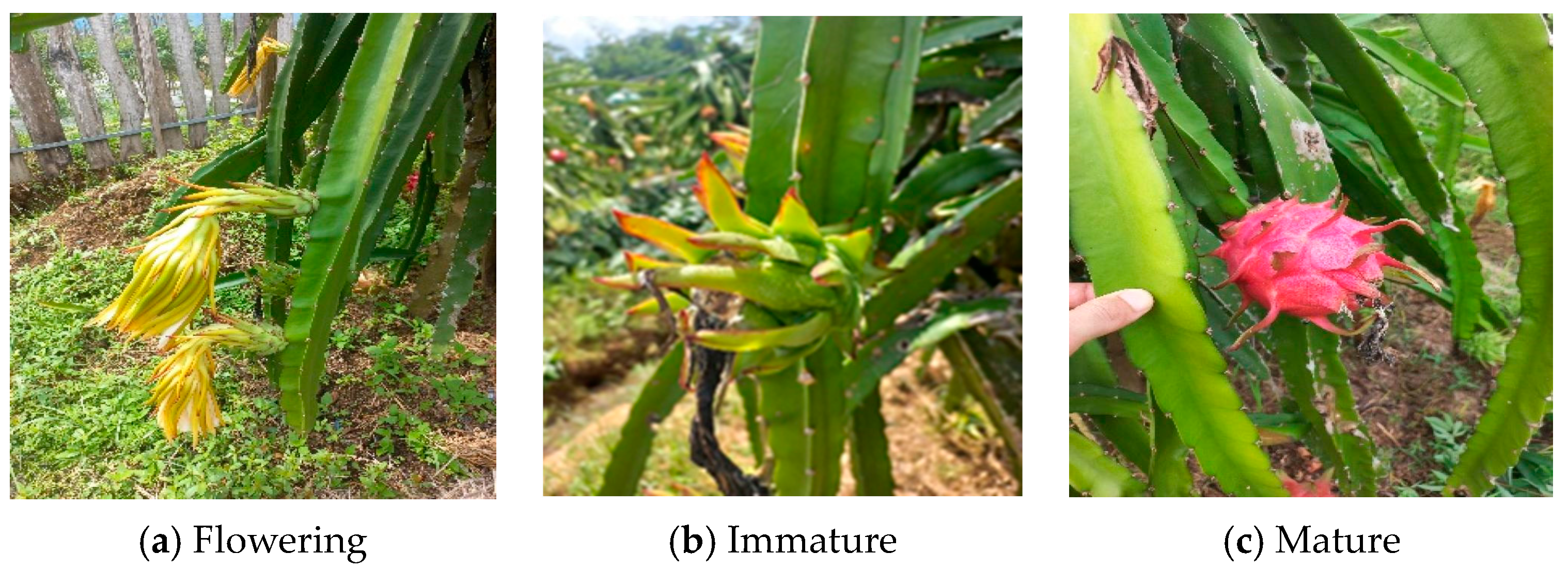
2.1. Construction of Data Sets

The present study involved the construction of a dataset comprising 1748 images of pitayas, which were used for the purposes of training and evaluating the YOLOv8n-CBN model. The images in the dataset were primarily sourced from the universe.roboflow website, which provides high-quality open-source image resources and image data for diverse scenes. Roboflow Universe is a computer vision community platform developed by Roboflow Inc., a company headquartered in Des Moines, IA, USA. The dataset is primarily comprised images sourced from this website, which accounts for approximately 60% of the total. Additionally, the dataset incorporates images from other online resources and field photography conducted by our team. We extend our gratitude to all contributors. We have ensured that the collection and utilisation of the dataset adhere to the relevant laws and regulations pertaining to copyright and data protection. Further details regarding the construction of the dataset and a comprehensive list of contributors can be found in the Appendix A.
The images in the dataset were classified into three categories: flowering, immature, and mature. Flowering pitayas have not yet formed fruit, which resemble long strips and appear yellow in colour (see Figure 1a). Ripening pitayas have fruit that are ripe and appear red in large areas (see Figure 1b). Unripe pitayas have formed fruit that appear green in colour (see Figure 1c). These images were saved in the .jpg format.
The dataset was annotated using the MakeSense tool, which generated the corresponding label files in .txt format. During the annotation process, fruit that are indistinguishable and ambiguous to the naked eye are not labelled. A Python 3.9 script was employed to randomly divide the dataset into three subsets: a training set (1223 images), a validation set (349 images), and a test set (176 images). The ratio of the three subsets was 7:2:1. The training set was employed to train the model, the validation set was utilised to adjust the hyperparameters of the model and conduct a preliminary assessment of the model’s capability, and the test set was used to test the model’s detection accuracy and assess its generalisation capability.

2.2. Methods

The process of the YOLOv8n-CBN detection system for pitaya growth status based on the improved YOLOv8 network structure is shown in Figure 2.

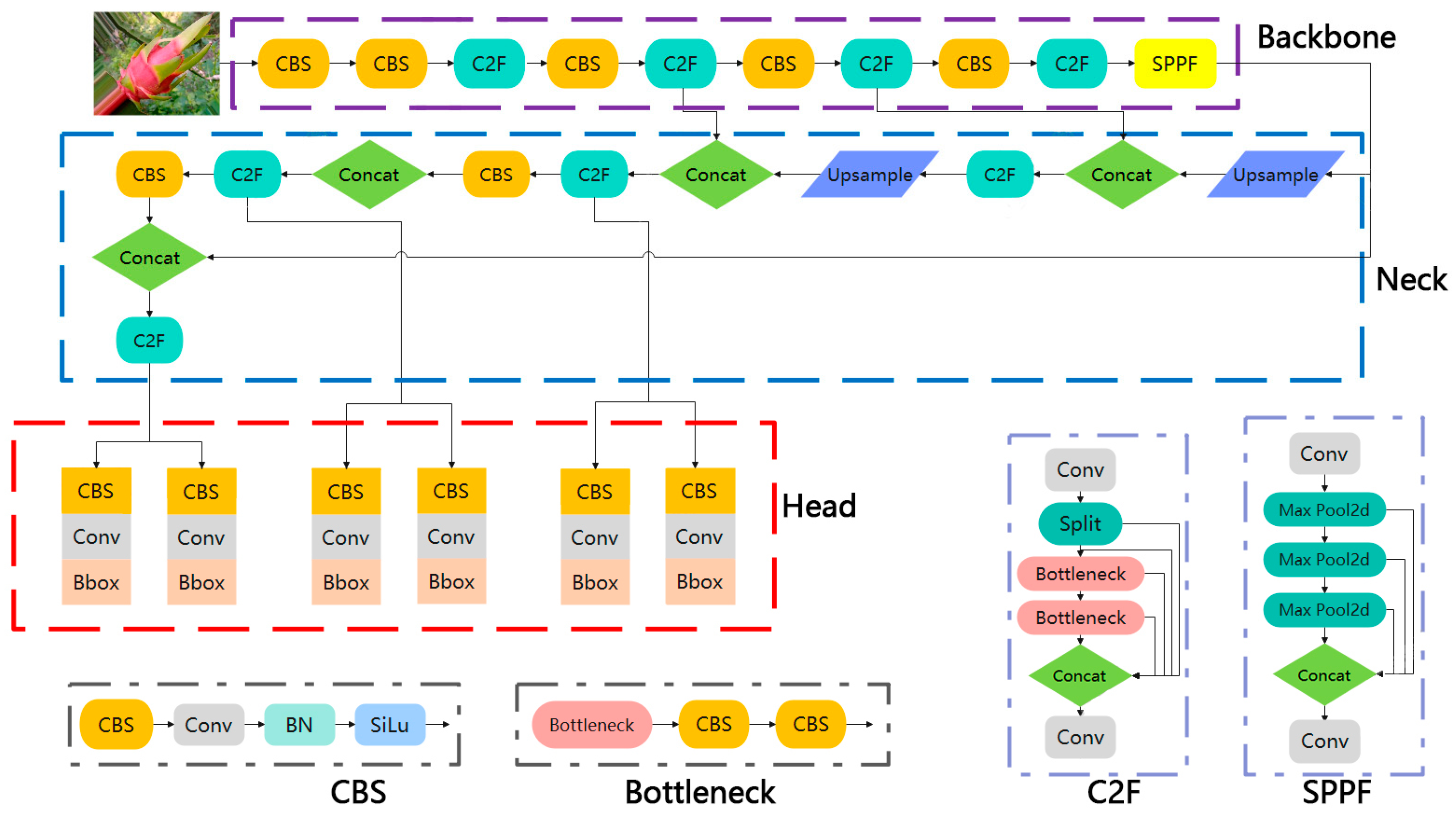
2.2.1. YOLOv8n Network Structure

The primary components of the YOLOv8 target detection algorithm are divided into three sections: Backbone, Head, and Neck [13]. The Backbone is responsible for the extraction of features from the input data and their subsequent transmission to the subsequent layers, where they are employed in the performance of the task. The Head is responsible for mapping the features extracted from the Backbone network to the task-related outputs. The role of the Neck is to further process the features extracted from the Backbone network and prepare them for use in the Head for a particular task. The network structure of YOLOv8n is depicted in Figure 3.
It should be noted that BN represents a batch normalization operation, SiLu is the activation function, Split is a slicing operation, Conv represents a convolution operation, Concat is the feature connection module, SPPF represents the spatial pyramid pooling module, Max pool2d represents the maximum pooling, Bbox represents the bounding box loss, and Cls represents the classification loss [14,15,16,17].

2.2.2. CBAM Attentional Mechanisms

CBAM is an attention mechanism module designed to enhance the performance of convolutional neural networks [18]. The primary objective of CBAM is to enhance the perceptual capabilities of the model by incorporating channel and spatial attention mechanisms into the convolutional neural network. The CBAM attention mechanism module is capable of enhancing the performance of the model without increasing the complexity of the network. The channel attention module is employed to assign weights to input channel feature maps, while the spatial attention module is used to assign weights to input spatial feature maps. The structure of the CBAM attention mechanism is shown in Figure 4.
The principal objective of the channel attention module is to enhance the feature representation of each channel. For the input features, the features are first fed into the pooling layer [19], which reduces the number of features in the network layer through global maximum pooling and global average pooling operations. This can suppress overfitting to some extent. The average pooling layer is employed to calculate the mean value of the image region during forward propagation, and the features are distributed evenly across the region during backward propagation. The application of average pooling allows for the suppression of image noise, the retention of a substantial quantity of image texture information for the purpose of feature classification, and the retention of a greater quantity of image background information. The average pooling process is shown in Figure 5.
In the maximum pooling layer, the maximum value of the image region is selected as the pooling value in forward propagation, and the maximum value is retained in backward propagation. The values of other positions are set to 0. Maximum pooling eliminates a significant amount of redundant information, but also results in the loss of a considerable amount of image detail. Consequently, edge information is typically retained in this manner. The maximum pooling process is shown in Figure 6.
The feature vectors resulting from global average pooling and global maximum pooling are input to a fully connected layer MLP. This fully connected layer is considered to be involved in training the model, along with the convolutional basis. The fully connected layer learns the weights of each channel, classifies the features, and decides which channel’s result is more important for learning. It then intersects the feature vectors and finally outputs the weights. A sigmoid activation function is added to the output vectors, as this is a necessary component of a neural network. Without an activation function in the hidden layers, the added layers are meaningless. For our dichotomous function, a sigmoid function is used. This maps values between 0 and 1, and the function values can be interpreted as mathematical probabilities. The addition of the sigmoid activation function allows weights to be applied to each channel of the image. Finally, integration is performed by multiplying the weights obtained by the original image features, re-adjusting the importance of each channel, and feeding the resulting feature map into the spatial attention module for the next step.
The spatial attention module is primarily concerned with identifying the most crucial regions within the feature image. This is achieved by first obtaining the feature image from the channel attention module and then averaging and maximally pooling it. This process yields two distinct channels, which are then spliced to generate two feature vector maps. Finally, the two maps are compressed to form a single channel, which is then convolved with a weight derived from the channel attention module. This weight is then activated by a sigmoid function, a process that is largely analogous to the aforementioned channel attention module. The maps are compressed to form a one-unit channel, and a convolution of quantity 1 is carried out to obtain the spatial attention weight, which is then activated by a sigmoid function. This step and the above channel attention module are largely the same, and will not be expanded in detail in this paper. Subsequently, the output weights are constrained to a range of (0, 1) through the application of a sigmoid activation function. Finally, the obtained weights are multiplied with the original image features to weight each spatial feature.

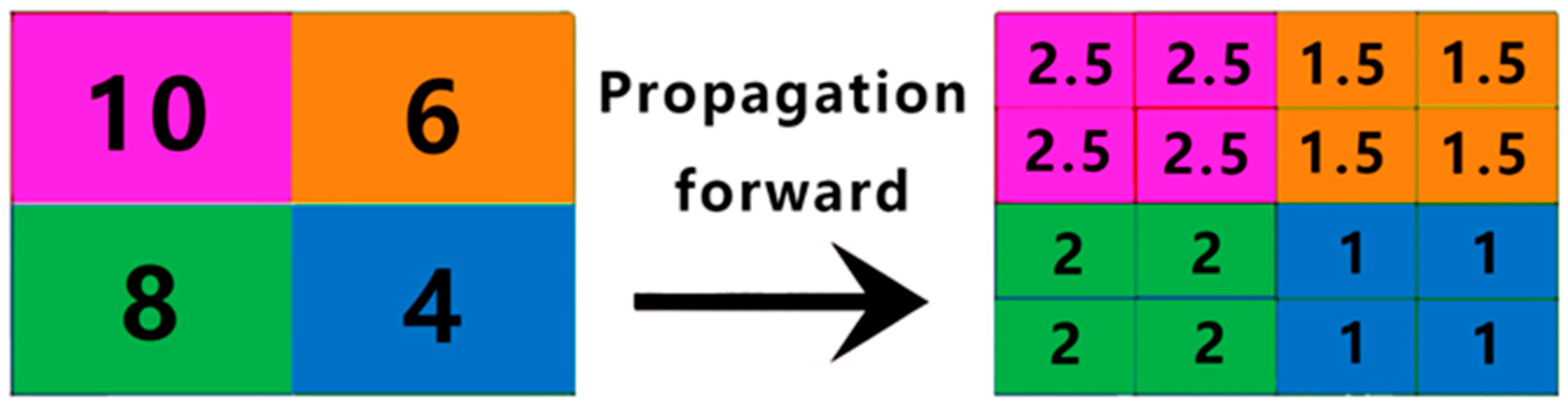
2.2.3. The BiFPN Network

The BiFPN network is an object detection neural network architecture derived from the Path Aggregation Network (PAnet) [20]. Employing a bidirectional pyramid structure, it facilitates simultaneous upward and downward feature fusion. Through iterative processes, it effectively enhances the quality of feature maps and extracts multi-scale object information. YOLOv8 utilizes an enhanced network that refines the feature pyramid network (FPN + PAN) by incorporating bottom-up paths, thereby bolstering target detection capabilities, particularly for small-scale targets [21]. However, the BiFPN network outperforms FPN + PAN in detecting small objects due to its more sophisticated feature fusion strategy. In PAN-FPN, the transmission of features through an increased number of layers within the network may result in the loss of fine details, particularly in deep feature maps. BiFPN’s bidirectional architecture captures additional contextual information through two-way feature exchange, thereby enhancing the efficiency of feature propagation within the network and consequently elevating the quality of feature representation. The architecture of BiFPN is depicted in Figure 7.
The circles represent features at varying scales, while the arrows illustrate the fusion of features across different scales. When examining the dark yellow circles in isolation, it can be discerned that the features are fused from top to bottom. Conversely, when considering the green circles in isolation, it is evident that the features are fused from bottom to top. Consequently, the feature fusion methodology employed by BiFPN is consistent and systematic.
BiFPN employs a rapid normalised fusion algorithm, whereby feature maps of disparate layers are merged by multiplying them with a learnable weight that is optimised by backpropagation during training [22]. This algorithm is frequently designated as weighted feature fusion [23]. The objective of weighted feature fusion is to facilitate the network’s capacity to automatically discern the significance of disparate input features and adjust their contribution to the ultimate fusion result in a corresponding manner. The fast normalised fusion algorithm is illustrated below:
p i t d = C o n v ω 1 × p i i n + ω 2 × R p i + 1 i n ω 1 + ω 2 + ϵ
p i o u t = C o n v ω 1 × p i i n + ω 2 × p i t d + ω 3 × R p i 1 i n ω 1 + ω 2 + ω 3 + ϵ
In the aforementioned algorithm, P i t d represents an intermediate feature of level i, P i o u t represents the output feature of level i, P i i n represents the input feature of level i, Conv represents a separable convolution, R denotes an upsampling or downsampling operation, and ω′ represents the weight associated with the learning process. The value of ϵ is extremely small and serves to guarantee the stability of the values in question; ω i refers to the weight of the input feature map.

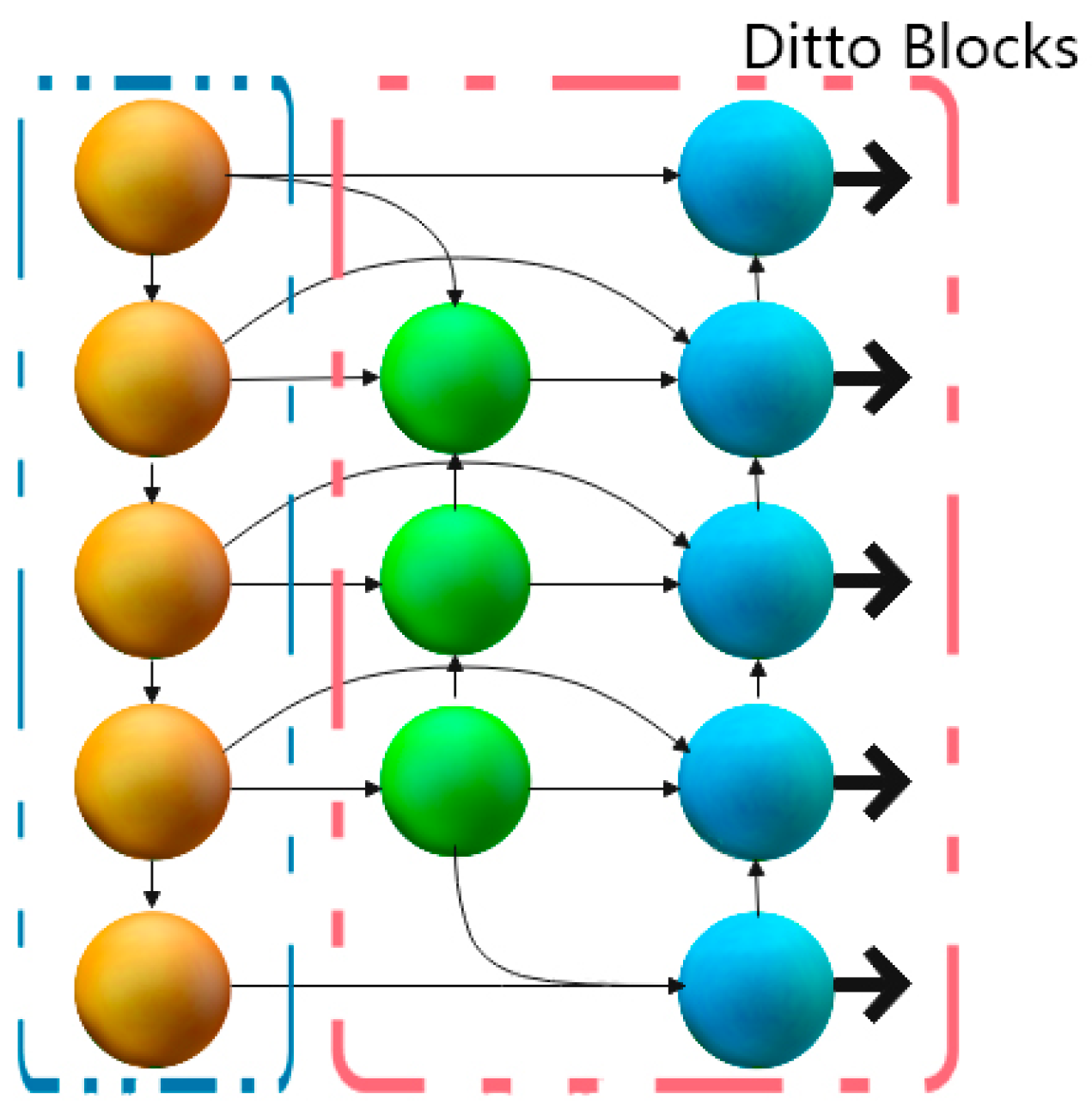
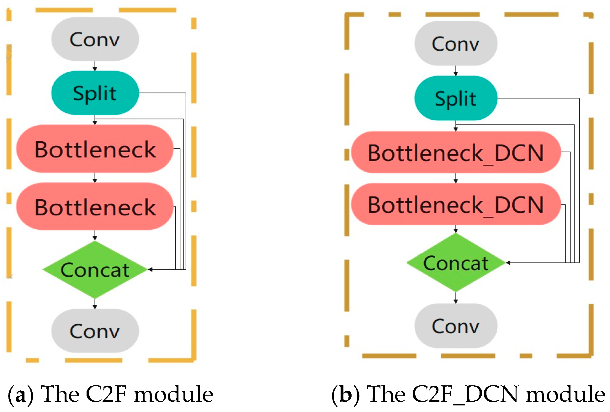
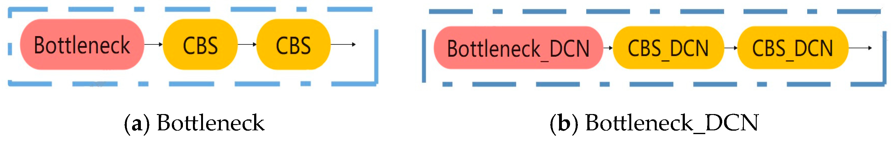
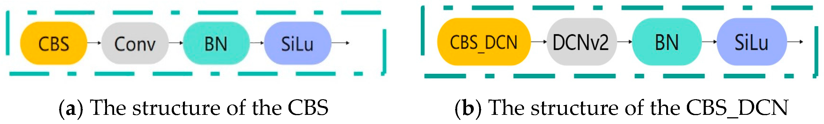
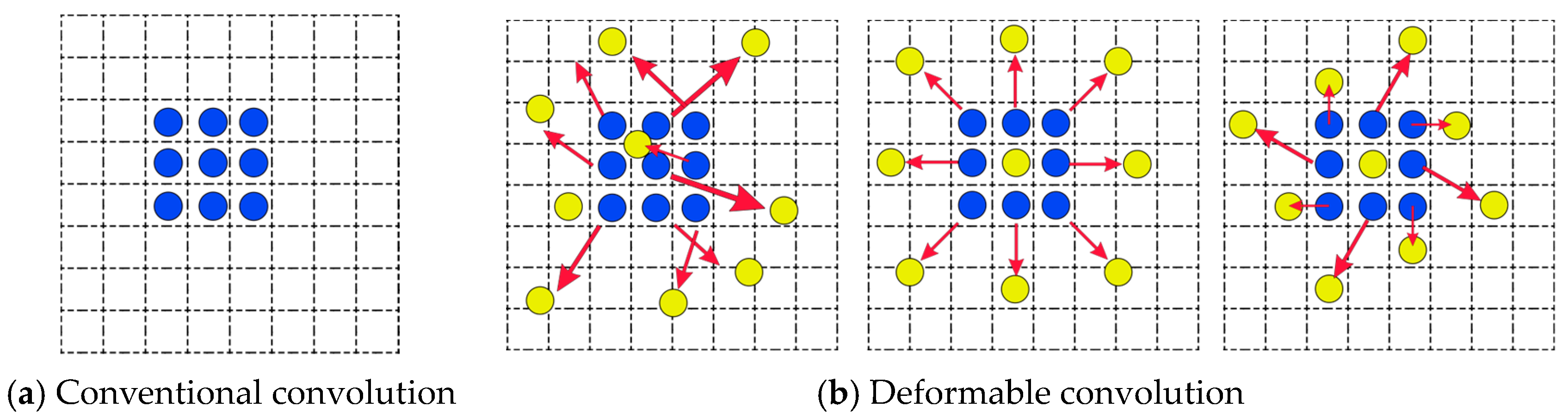
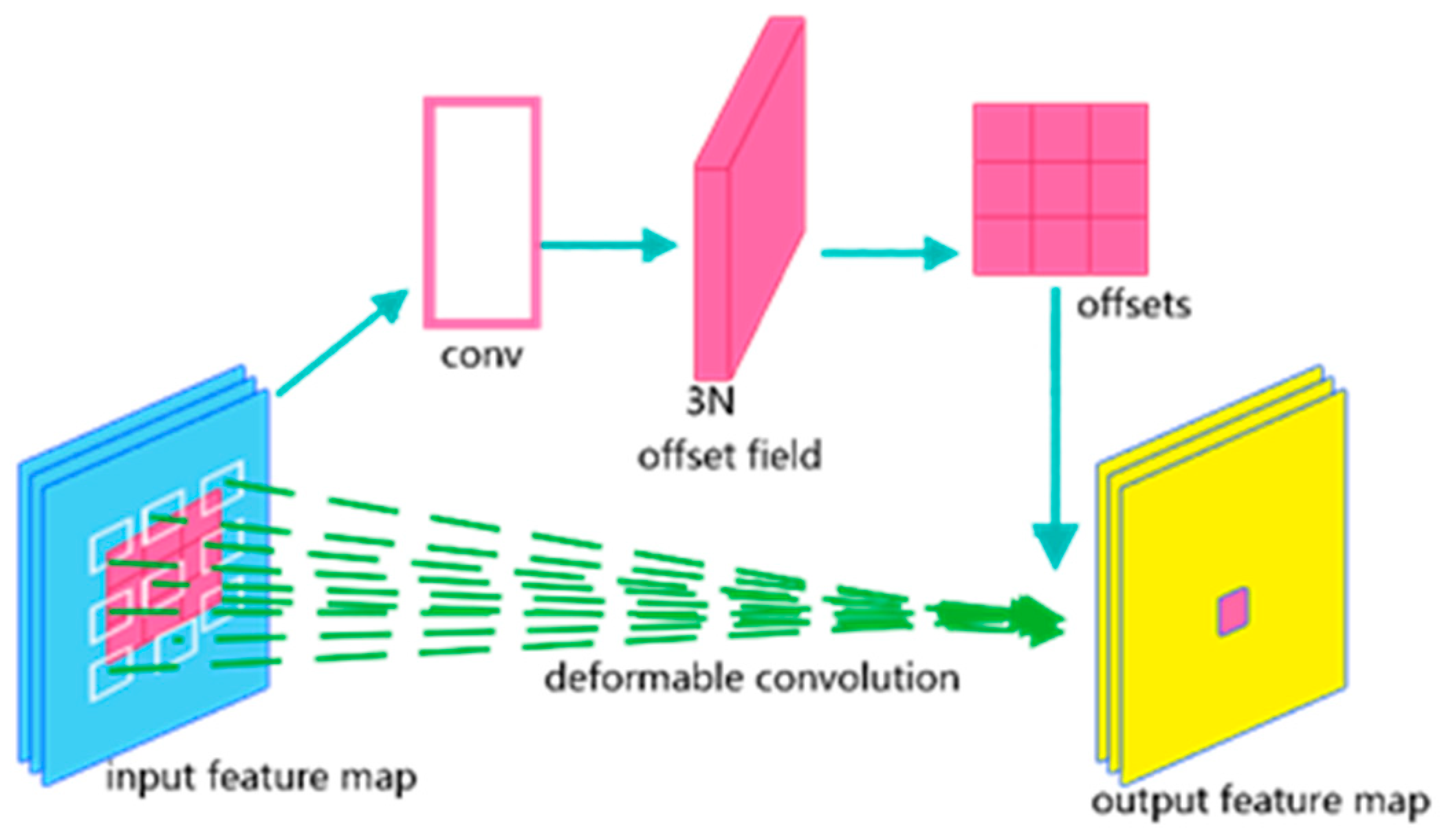
2.2.4. The C2F_DCN Module

The C2F_DCN module is based on the C2F module, which replaces the Bottleneck module with the Bottleneck_SCN module [24]. The structures of the C2F module and the C2F_DCN module are depicted in Figure 8. In the C2F module, the input data are initially subjected to a convolutional processing stage, which is then followed by a Split processing stage. Subsequently, the data are processed by the Bottleneck module, and finally, the outputs of the residual module and the Backbone module are concatenated and subjected to a convolutional processing stage for output generation [25]. The residual module comprises a Split and subsequent Concat stage.
The Bottleneck module is comprised two CBS modules, whereas the Bottleneck_DCN module is based on the Bottleneck module, with the CBS module replaced by the CBS_DCN module. The Bottleneck module initially passes through one CBS module and subsequently proceeds to pass through the other CBS module. The structures of the Bottleneck module and the Bottleneck_DCN module are depicted in Figure 9.
The CBS module comprises a convolutional layer, a BatchNorm2d layer, and a SiLU activation function [26]. The CBS_DCN module is based on the CBS module, which replaces the convolutional layer with DCNv2 (a deformable convolution). In the CBS module, the input is initially processed by the convolutional layer, then normalised by BN (BatchNorm), and finally activated by the SiLU function. In the CBS module, the input is initially processed by the convolutional layer, then normalised by the batch normalisation (BN) layer, and finally by the SiLU activation function. The structures of the CBS and CBS_DCN modules are depicted in Figure 10.
DCNv2, or Deformable Convolutional Networks Version 2, represents an enhanced iteration of the original Deformable Convolutional Networks (DCN) model [27]. It has been optimised and extended from the DCN foundation, incorporating advancements in convolutional network design. Deformable convolution entails the introduction of an offset to the sampling position in the standard convolution operation. This enables the model to adaptively adjust the sampling position of the convolution kernel, thereby facilitating a more optimal accommodation of changes in image content. In conventional convolution, the sampling is performed with a fixed grid, as illustrated in Figure 11a. Consequently, traditional convolution is unable to adapt to alterations in the target shape and pose when dealing with targets exhibiting complex geometric variations, resulting in inaccurate feature extraction for small, occluded or truncated targets. Furthermore, traditional convolution is constrained in its capacity for feature fusion, typically only fusing features from fixed locations, which constrains the network’s comprehension of complex scenes. Figure 11b illustrates the deformable convolution sampling process. The sampling locations for deformable convolution are indicated by yellow dots with enhanced offsets (red arrows). Consequently, in comparison to traditional convolution, deformable convolution can enhance the model’s ability to localise and generalise to targets by adaptively adjusting the sampling points, particularly in target detection and segmentation tasks.
The structure of DCNv2 is illustrated in Figure 12. Initially, a set of prediction results for convolution kernel offsets is input following a conventional convolution operation [28]. Subsequently, the offset field is traversed in order to obtain the bias field of the convolution kernel sampling points. This enables the convolution kernel to learn the offsets in the x and y directions, respectively. Consequently, the bias matrix of the convolution kernel sampling points is obtained, and thus the offsets p n are obtained. Ultimately, the convolution kernel structure of the feature map is optimised using bilinear interpolation methods. Figure 12 illustrates that the number of channels for the offset is 3N, where 3 refers to the offset in the x-direction and the offset in the y-direction, as well as the value of the penalty parameter m k . In comparison to DCNv1, the number of channels utilized for the prediction result has been modified from the initial 2N to 3N. This alteration is attributed to the incorporation of an additional parameter in DCNv2 for learning purposes, namely the penalty parameter, m k . The value of N represents the number of pixels within the convolution kernel [29].
The formula for DCNv2 at a given sampling point is as follows:
y p o = p o R ω p n x p o + p n + p n m k
In Equation (3), the notation y p o is used to denote the value of p o at each position of y in the output feature map. The notation ω p n is used to denote the weights of the convolutional kernel at p n ; p n is an element in R, where R denotes the size of the sensory field. For example, R{(1, 1), (1, 0), … (1, 1)} denotes a 3 × 3 convolutional kernel. The variable x is used to denote the position of the feature map, x p o + p n + p n . The offset added at the traditional convolutional sampling points with added offsets is represented by the variable p n . The penalty parameter, denoted by the variable m k , is a decimal between 0 and 1.
The bilinear interpolation formula is defined as follows:
x p = G q , p x q
In Equation (4), the symbol x(p) denotes the pixel value that has been calculated by means of interpolation. The variable p represents an arbitrary position within the offset region, which is defined as ( p = p o + p n + p n ). The symbol q denotes the spatial position of the input feature mapping, while the function G q , p represents the bilinear interpolation function for a single 2D convolutional kernel [30].

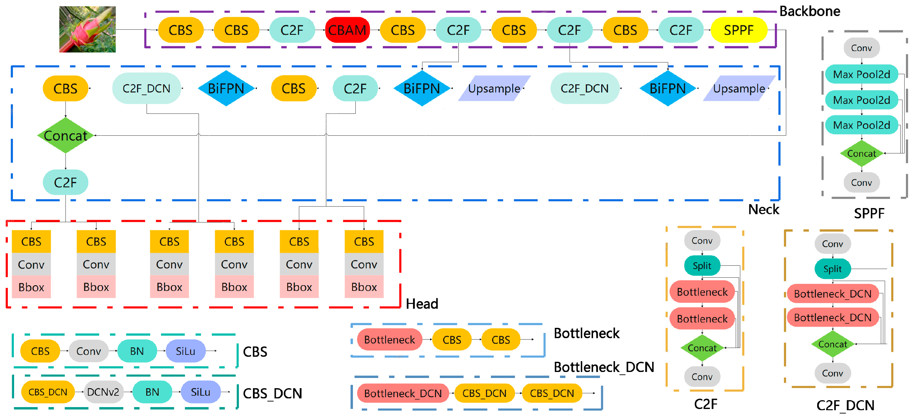
2.2.5. YOLOv8n-CBN Network Architecture

The proposed modification to the YOLOv8n model entails the incorporation of the CBAM attention mechanism into its network structure. This could be theoretically implemented after each convolutional block in the Backbone network. The CBAM attention mechanism module was incorporated subsequent to the initial C2F module (layer 3) within the Backbone section. The objective of incorporating CBAM into the YOLOv8n model is to enhance detection accuracy for complex scenes and small targets. Secondly, the BiFPN mechanism is incorporated into the feature enhancement module. The objective is to facilitate the more effective capture of multi-scale features and enhance the efficiency of feature information transfer within the network. Ultimately, a number of the C2F modules present in the Neck section have been substituted with C2f_DCN. The network structure of YOLOv8n-CBN is illustrated in Figure 13.

3. Results and Discussion

3.1. Experimental Environment

The experimental environment was conducted using PyCharm Community Edition 2023.2.3, on a laptop with an NVIDIA GeForce RTX 3060 GPU with 24 GB of video memory. The programming language was Python 3.9.18, with CUDA v118 used to accelerate the GPU, and the deep learning framework PyTorch 2.0.1 was employed.

3.2. Ablation Experiment

To assess the efficacy of the aforementioned improvements, ablation experiments were conducted to compare the effects before and after the implementation of the improvements. The evaluation metrics employed were precision (P), recall (R), F1 score (F1), average precision mean ([email protected]) at an IoU threshold of 0.50, average precision mean ([email protected]–0.95) at different IoU thresholds, inference time, and model size (weight), which are defined in Equations (5)–(9).
P = T P F P + T P
R = T P F N + T P
A P = 0 1 P ( R ) d R
F 1 = 2 P · R P + R
m A P = i = 0 n A P ( i ) n
In the aforementioned equation, TP represents the number of correctly identified targets, FP denotes the number of targets that the detector erroneously identifies as targets but which are, in fact, non-targets, and FN signifies the number of non-targets that the detector incorrectly identifies as targets.
In order to ascertain the influence of each enhanced module on the model, we conducted ablation experiments and compared the original YOLOv8n model with a series of modified iterations. The results of the aforementioned ablation experiment are presented in tabular form in Table 1.
As illustrated in Table 1, the precision and recall rates have been enhanced by 3.1% and 3.8%, respectively, in comparison to the preceding values following the implementation of the proposed modifications. Additionally, the [email protected] and [email protected]–0.95 values have exhibited an improvement of 2.1% and 1.2%, respectively. This implies that the enhanced model will diminish the occurrence of leakage and erroneous detection in the process of pitaya growth detection. Additionally, we observed that following the replacement of the C2F-DCN module, the inference time increased, and the size of the weight file for the model increased by 0.2 MB compared to the pre-improvement period. This is attributed to the introduction of additional offset parameters by the deformable convolution, which resulted in an increase in the storage and computational requirements of the model.

3.3. Performance Comparison of Different Models

A performance comparison is conducted between the improved YOLOv8n-based YOLOv8n-CBN algorithms and the target detection algorithms of YOLOv3-tiny, YOLOv5s, YOLOv5m, and YOLOv8n. The training set of the dataset was first subjected to training in YOLOv3-tiny, YOLOv5s, YOLOv5m, and YOLOv8n. Subsequently, the weight files trained by each of the aforementioned models were obtained and incorporated into the validation set for verification. Ultimately, the data presented in Table 2 were generated.
In comparison to the YOLOv3-tiny model, the YOLOv8n-CBN model demonstrated an 8.8% improvement in precision, a 6.3% improvement in recall, a 7.5% improvement in F1 score, a 6.7% improvement in [email protected], and a 10.5 MB reduction in weight. Additionally, the [email protected]–0.95 metric exhibited a 10.1% enhancement. In terms of inference time, the YOLOv8n-CBN model is observed to exhibit a slight increase of 2.5 ms in comparison to YOLOv3-tiny.
A reduction of 4.1% has been observed in the recall of the YOLOv8n-CBN model in comparison to the YOLOv5s. Furthermore, the inference time of YOLOv8n-CBN is extended by 0.7 ms. However, in terms of precision, F1 score, [email protected], and [email protected]–0.95, the YOLOv8n-CBN model outperforms the YOLOv5s model by 5.2%, 0.5%, 0.7%, and 5.0%, respectively. Additionally, the YOLOv8n-CBN model is 7.7 MB smaller in terms of weight than the YOLOv5s model.
In comparison to the YOLOv5m model, the YOLOv8n-CBN model demonstrates a 3.9% enhancement in precision, a 2.9% reduction in recall, and a 0.4% increase in F1 score. The [email protected] value increased by 0.5%, while the [email protected]–0.95 value increased by 1.6%. Additionally, there was a reduction in inference time of 5.2 ms and a reduction in weight of 34.4 MB.
As can be seen in Table 2, the [email protected] value for YOLOv8n-CBN is 0.911, which is lower than the value reported by some research scholars in the Introduction section. The discrepancy can be attributed to the fact that the detected targets are not identical. The target of their detection is the ripe pitaya, which is bright red in a large area and exhibits a significant contrast with the background environment. Consequently, the detection is more precise, and there are minimal instances of missed recognition. Conversely, the targets of our model are the three stages of pitaya growth, in which the unripe pitaya is situated in closer proximity to the environment due to its green colour, thus rendering it more susceptible to misrecognition during the recognition process. Consequently, the enhancements we have implemented continue to possess a certain degree of significance, despite the fact that our proposed model exhibits a lower mAP value than those proposed by certain researchers in the Introduction section.
In conclusion, the YOLOv8n-CBN model demonstrates greater overall superiority than the aforementioned models. Consequently, it is more effective at accurately detecting the growth status of dragon fruit in complex natural environments.

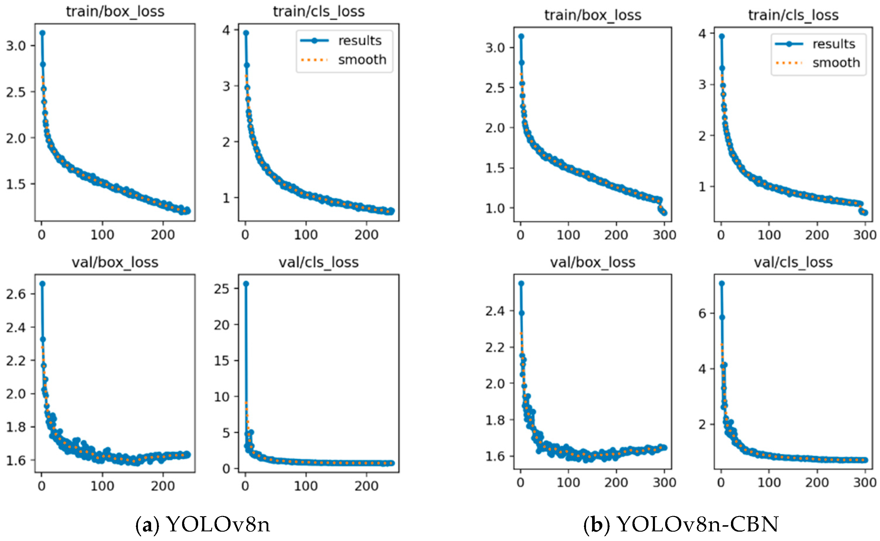
3.4. A Comparative Analysis of the Loss Function Prior to and following Improvement

In order to observe the performance difference between the YOLOv8n-CBN model and the YOLOv8n model, and to verify whether the YOLOv8n-CBN model underfitted or overfitted during training and validation, we recorded the loss functions of the YOLOv8n-CBN model and the YOLOv8n model during training and validation. The results are presented in Figure 14.
Figure 14 illustrates that the loss function changes exhibited by the YOLOv8n and YOLOv8n-CBN models are largely similar. It can thus be concluded that the stability and robustness of the YOLOv8n model, both before and after the improvement, are essentially identical. Furthermore, it can be observed that neither model exhibits the phenomenon of “low loss function in the training set, but high loss function in the validation set”. Instead, the loss functions of the training sets for both models demonstrate convergence and gradually approach a smooth trajectory. This suggests that neither model is subject to overfitting nor underfitting.

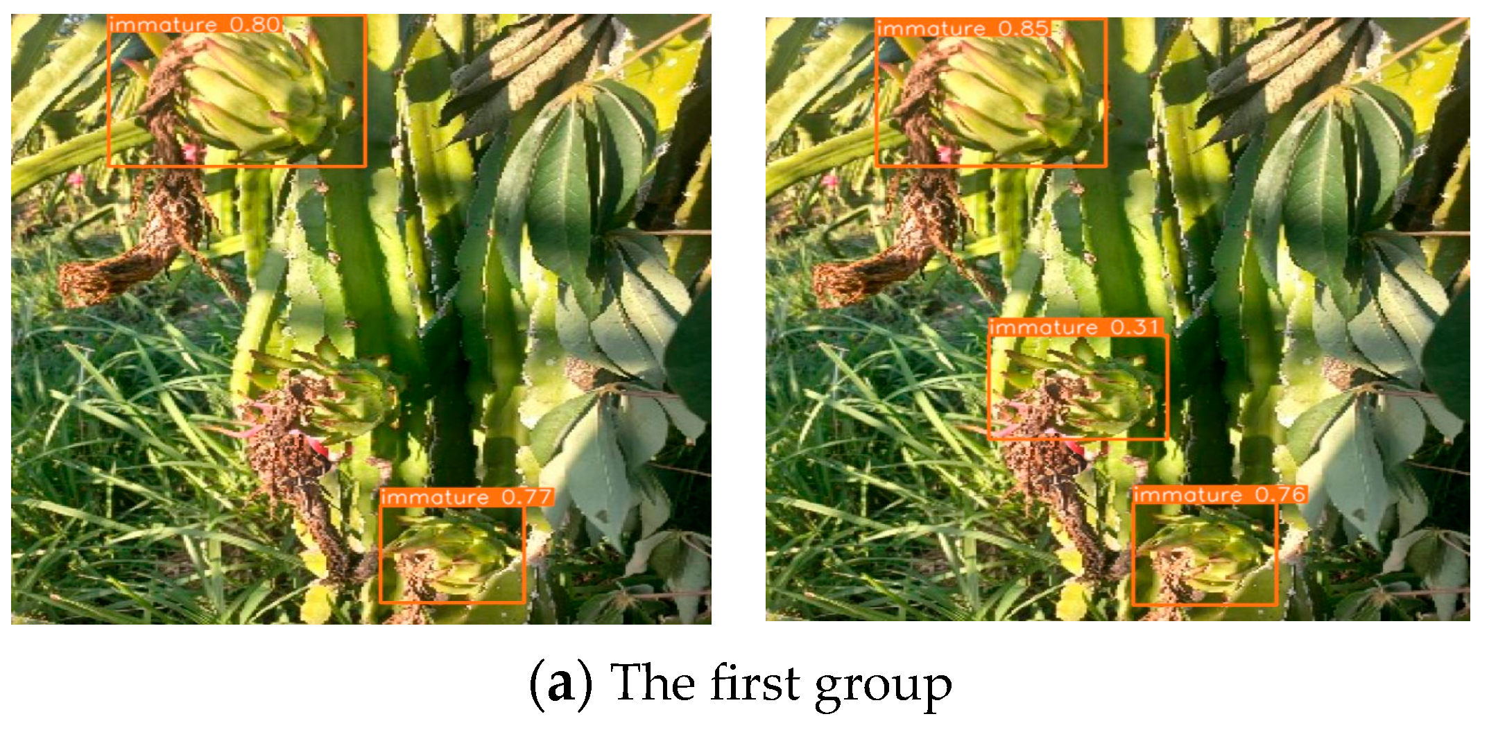
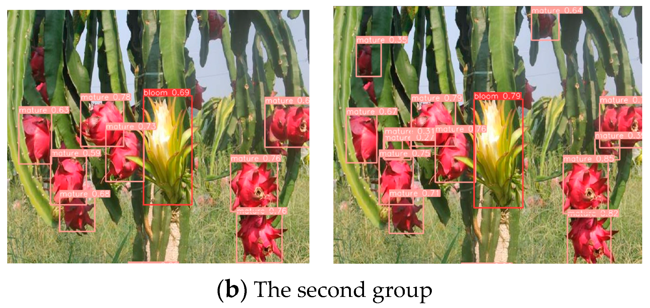
3.5. Comparison of the Growth State of Pitaya Fruit Results before and after the Improved Model

In order to observe the impact of the models prior to and following the implementation of enhancements on the detection of pitaya growth state, we have utilised the YOLOv8n and YOLOv8n-CBN models on the same pitaya growth state images, as illustrated in Figure 15.
Figure 15 presents a comparison of two groups of pitaya detection results, each comprising two images. The images on the left were obtained using the YOLOv8n model, while those on the right were obtained using the YOLOv8n-CBN model. It can be observed from the initial set of results that the YOLOv8 model has exhibited a tendency to misjudge the detection of the blurrier pitaya, whereas the YOLOv8-CBN model has demonstrated a higher degree of accuracy in this regard. From the second group, it can be observed that the YOLOv8-CBN model is capable of accurately identifying obscured pitayas, whereas the YOLOv8n model is prone to the phenomenon of missed judgement in such instances. It can thus be concluded that the YOLOv8-CBN model outperforms the YOLOv8n in terms of avoiding the phenomenon of missed judgement.

4. Conclusions

In order to enhance the efficacy of pitaya detection in complex natural environments, which are prone to false negatives and false positives, we have developed an enhanced model, YOLOv8-CBN. This is based on the YOLOv8n network model and is designed to detect the three growth stages of pitaya: flowering, immature, and ripe. This model represents a significant advancement over previous studies in this field, with the following key contributions:
The YOLOv8n-CBN model incorporates a CBAM attention mechanism module, fuses a BiFPN network, and replaces a portion of the C2F module with the C2F_DCN module. The experimental results demonstrate that the method enhances the network’s ability to extract features and the efficiency of transferring network feature information. Ultimately, [email protected] reached 91.1%, and the F1 score reached 87.6%. In comparison to the current mainstream models of YOLOv3-tiny, YOLOv5s, YOLOv5l, and YOLOv8n, this model demonstrates superior performance. While there is a discrepancy in the mAP value between this model and those proposed by some individuals in the introduction, this is unavoidable given that the detection targets are not identical. Consequently, this model can be effectively applied to detect the growth status of pitayas in a natural environment.
The YOLOv8-CBN model demonstrates remarkable efficacy in discerning the growth status of pitayas. For agricultural producers, it offers a valuable tool for real-time monitoring of plant development and the identification of unripe fruits, facilitating more efficient and informed decision-making regarding crop management. It is therefore evident that this study has significant implications for the advancement of intelligent techniques in agricultural operations.

Author Contributions

Conceptualization, Z.Q. and X.T. (Xinyuan Tian); methodology, S.Z.; software, X.T. (Xuejun Tian); validation, M.L., F.H. and X.T. (Xuejun Tian); formal analysis, S.Z.; investigation, M.L.; resources, X.T. (Xinyuan Tian); data curation, S.Z.; writing—original draft preparation, Z.Q.; writing—review and editing, S.Z.; visualization, D.M.; supervision, S.Z.; project administration, Z.Q.; funding acquisition, X.T. (Xinyuan Tian). All authors have read and agreed to the published version of the manuscript.

Funding

This research was funded by Research on Intelligent Monitoring Technology of Pitaya Growth Cycle Based on Machine Vision (Grant No. 2023ZDZX4031) and the Special Talent Fund of Lingnan Normal University (ZL22026).

Data Availability Statement

The original contributions presented in this study are included in the article; further inquiries can be directed to the corresponding author.

Conflicts of Interest

The authors declare no conflicts of interest.

Appendix A

The Primary Source of the Dataset: https://universe.roboflow.com/dragonfarm-aurrj/dragon_det (accessed on 21 December 2023).

References

  1. Khatun, T.; Nirob, M.A.S.; Bishshash, P.; Akter, M.; Uddin, M.S. A comprehensive dragon fruit image dataset for detecting the maturity and quality grading of dragon fruit. Data Brief 2023, 52, 109936. [Google Scholar] [CrossRef] [PubMed]
  2. Li, H.; Gu, Z.; He, D.; Wang, X.; Huang, J.; Mo, Y.; Li, P.; Huang, Z.; Wu, F. A lightweight improved YOLOv5s model and its deployment for detecting pitaya fruits in daytime and nighttime light-supplement environments. Comput. Electron. Agric. 2024, 220, 108914. [Google Scholar] [CrossRef]
  3. Zhou, J.; Zhang, Y.; Wang, A.J. A Dragon Fruit Picking Detection Method Based on YOLOv7 and PSP-Ellipse. Sensors 2023, 23, 3803. [Google Scholar] [CrossRef]
  4. Kenta, O.; Hiroki, Y. Comparison of the Noise Robustness of FVC Retrieval Algorithms Based on Linear Mixture Models. Remote Sens. 2011, 3, 1344–1364. [Google Scholar] [CrossRef]
  5. Kamilaris, A.; Prenafeta-Boldú, F.X. Deep learning in agriculture: A survey. Comput. Electron. Agric. 2018, 147, 70–90. [Google Scholar] [CrossRef]
  6. Liu, Z.; Wang, H. Automatic Detection of Transformer Components in Inspection Images Based on Improved Faster R-CNN. Energies 2018, 11, 3496. [Google Scholar] [CrossRef]
  7. Wang, X.; Hua, X.; Xiao, F.; Li, Y.; Hu, X.; Sun, P. Multi-Object Detection in Traffic Scenes Based on Improved SSD. Electronics 2018, 7, 302. [Google Scholar] [CrossRef]
  8. Ma, H.; Liu, Y.; Ren, Y.; Yu, J. Detection of Collapsed Buildings in Post-Earthquake Remote Sensing Images Based on the Improved YOLOv3. Remote Sens. 2019, 12, 44. [Google Scholar] [CrossRef]
  9. Redmon, J.; Farhadi, A. YOLOv3: An Incremental Improvement. arXiv 2018, arXiv:1804.02767. [Google Scholar]
  10. Wang, C.; Sun, W.; Wu, H.; Zhao, C.; Teng, G.; Yang, Y.; Du, P. A Low-Altitude Remote Sensing Inspection Method on Rural Living Environments Based on a Modified YOLOv5s-ViT. Remote Sens. 2022, 14, 4784. [Google Scholar] [CrossRef]
  11. Su, X.; Zhang, J.; Ma, Z.; Dong, Y.; Zi, J.; Xu, N.; Zhang, H.; Xu, F.; Chen, F. Identification of Rare Wildlife in the Field Environment Based on the Improved YOLOv5 Model. Remote Sens. 2024, 16, 1535. [Google Scholar] [CrossRef]
  12. Zhou, J.; Zhang, Y.; Wang, J. RDE-YOLOv7: An Improved Model Based on YOLOv7 for Better Performance in Detecting Dragon Fruits. Agronomy 2023, 13, 1042. [Google Scholar] [CrossRef]
  13. Yang, S.; Wang, W.; Gao, S.; Deng, Z. Strawberry ripeness detection based on YOLOv8 algorithm fused with LW-Swin Transformer. Comput. Electron. Agric. 2023, 215, 108360. [Google Scholar] [CrossRef]
  14. Qi, J.; Liu, X.; Liu, K.; Xu, F.; Guo, H.; Tian, X.; Li, M.; Bao, Z.; Li, Y. An improved YOLOv5 model based on visual attention mechanism: Application to recognition of tomato virus disease. Comput. Electron. Agric. 2022, 194, 106780. [Google Scholar] [CrossRef]
  15. Lan, K.; Jiang, X.; Ding, X.; Lin, H.; Chan, S. High-Efficiency and High-Precision Ship Detection Algorithm Based on Improved YOLOv8n. Mathematics 2024, 12, 1072. [Google Scholar] [CrossRef]
  16. Jing, J.; Li, S.; Qiao, C.; Li, K.; Zhu, X.; Zhang, L. A tomato disease identification method based on leaf image automatic labeling algorithm and improved YOLOv5 model. J. Sci. Food Agric. 2023, 103, 7070–7082. [Google Scholar] [CrossRef]
  17. Zhou, Y.; Zhu, W.; He, Y.; Li, Y. YOLOv8-based Spatial Target Part Recognition. In Proceedings of the 2023 IEEE 3rd International Conference on Information Technology, Big Data and Artificial Intelligence (ICIBA), Chongqing, China, 26–28 May 2023; Volume 3, pp. 1684–1687. [Google Scholar]
  18. Ayaz, I.; Kutlu, F.; Cömert, Z. DeepMaizeNet: A novel hybrid approach based on CBAM for implementing the doubled haploid technique. Agron. J. 2023, 116, 861–870. [Google Scholar] [CrossRef]
  19. Liu, W.; Wang, Z.; Liu, X.; Zeng, N.; Liu, Y.; Alsaadi, F.E. A survey of deep neural network architectures and their applications. Neurocomputing 2017, 234, 11–26. [Google Scholar] [CrossRef]
  20. Touko Mbouembe, P.L.; Liu, G.; Park, S.; Kim, J.H. Accurate and fast detection of tomatoes based on improved YOLOv5s in natural environments. Front. Plant Sci. 2024, 14, 1292766. [Google Scholar] [CrossRef]
  21. Wang, Z.; Ma, B.; Li, Y.; Li, R.; Jia, Q.; Yu, X.; Sun, J.; Hu, S.; Gao, J. Concurrent Improvement in Maize Grain Yield and Nitrogen Use Efficiency by Enhancing Inherent Soil Productivity. Front. Plant Sci. 2022, 13, 790188. [Google Scholar]
  22. Zhu, R.; Wang, X.; Yan, Z.; Qiao, Y.; Tian, H.; Hu, Z.; Zhang, Z.; Li, Y.; Zhao, H.; Xin, D.; et al. Exploring Soybean Flower and Pod Variation Patterns During Reproductive Period Based on Fusion Deep Learning. Front. Plant Sci. 2022, 13, 922030. [Google Scholar] [CrossRef]
  23. Wang, Q.; Zheng, W.; Wu, F.; Xu, A.; Zhu, H.; Liu, Z. A New GNSS-R Altimetry Algorithm Based on Machine Learning Fusion Model and Feature Optimization to Improve the Precision of Sea Surface Height Retrieval. Front. Earth Sci. 2021, 9, 730565. [Google Scholar] [CrossRef]
  24. Pan, P.; Shao, M.; He, P.; Hu, L.; Zhao, S.; Huang, L.; Zhou, G.; Zhang, J. Lightweight cotton diseases real-time detection model for resource-constrained devices in natural environments. Front. Plant Sci. 2024, 15, 1383863. [Google Scholar] [CrossRef]
  25. Mbouembe, P.L.T.; Liu, G.; Sikati, J.; Kim, S.C.; Kim, J.H. An efficient tomato-detection method based on improved YOLOv4-tiny model in complex environment. Front. Plant Sci. 2023, 14, 1150958. [Google Scholar] [CrossRef] [PubMed]
  26. Wang, X.; Cao, Y.; Wu, S.; Yang, C. Real-time detection of deep-sea hydrothermal plume based on machine vision and deep learning. Front. Mar. Sci. 2023, 10, 1124185. [Google Scholar] [CrossRef]
  27. Liu, M.; Li, R.; Hou, M.; Zhang, C.; Hu, J.; Wu, Y. SD-YOLOv8: An Accurate Seriola dumerili Detection Model Based on Improved YOLOv8. Sensors 2024, 24, 3647. [Google Scholar] [CrossRef] [PubMed]
  28. Wang, F.; Jiang, J.; Chen, Y.; Sun, Z.; Tang, Y.; Lai, Q.; Zhu, H. Rapid detection of Yunnan Xiaomila based on lightweight YOLOv7 algorithm. Front. Plant Sci. 2023, 14, 1200144. [Google Scholar] [CrossRef] [PubMed]
  29. He, C.; Wan, F.; Ma, G.; Mou, X.; Zhang, K.; Wu, X.; Huang, X. Analysis of the Impact of Different Improvement Methods Based on YOLOV8 for Weed Detection. Agriculture 2024, 14, 674. [Google Scholar] [CrossRef]
  30. Ping, X.; Yao, B.; Niu, K.; Yuan, M. A Machine Learning Framework with an Intelligent Algorithm for Predicting the Isentropic Efficiency of a Hydraulic Diaphragm Metering Pump in the Organic Rankine Cycle System. Front. Energy Res. 2022, 10, 851513. [Google Scholar] [CrossRef]
Figure 1. Partial images of the pitaya dataset.
Horticulturae 10 00899 g001
Figure 2. Flowchart of pitaya growth status detection system.
Horticulturae 10 00899 g002
Figure 3. Network structure diagram of YOLv8n.
Horticulturae 10 00899 g003
Figure 4. Structure diagram of CBAM attention mechanism.
Horticulturae 10 00899 g004
Figure 5. Average pooling process diagram.
Horticulturae 10 00899 g005
Figure 6. Maximum pooling process diagram.
Horticulturae 10 00899 g006
Figure 7. The schematic diagram of the BiFPN structure.
Horticulturae 10 00899 g007
Figure 8. The structure diagram of the C2F module and the C2F_DCN module.
Horticulturae 10 00899 g008
Figure 9. The structure of the Bottleneck module and the Bottleneck_DCN module.
Horticulturae 10 00899 g009
Figure 10. The structure of the CBS and CBS_DCN modules.
Horticulturae 10 00899 g010
Figure 11. The principles of both conventional convolution and variable convolution.
Horticulturae 10 00899 g011
Figure 12. The schematic diagram of the DCNv2 structure.
Horticulturae 10 00899 g012
Figure 13. Network structure diagram of YOLOv8n-CBN.
Horticulturae 10 00899 g013
Figure 14. The loss functions of the YOLOv8n-CBN model and the YOLOv8n model.
Horticulturae 10 00899 g014
Figure 15. Comparison of test results of pitaya growth state before and after YOLOv8n improvement.
Horticulturae 10 00899 g015aHorticulturae 10 00899 g015b
Table 1. Ablation experiment.
NoneCBAMBiFPNC2F-DCNPRF1mAP
@0.5
mAP
@0.50–0.95
Inference
Time
Weight
0.8800.8050.8420.8900.4705.6 ms6.2 MB
0.8950.8530.8730.9050.4775.6 ms6.2 MB
0.8810.8540.8670.9110.4765.8 ms6.2 MB
0.8930.8350.8630.9020.4786.3 ms6.4 MB
0.9110.8430.8760.9110.4826.4 ms6.4 MB
Table 2. Performance comparison of different models.
YOLOv3-TinyYOLOv5sYOLOv5mYOLOv8nYOLOv8n-CBN
P0.8230.8590.8720.8800.911
R0.7800.8840.8720.8050.843
F10.8010.8710.8720.8420.876
[email protected]0.8440.9040.9060.8900.911
[email protected]–0.950.3810.4320.4660.4700.482
inference time3.9 ms5.7 ms11.6 ms5.6 ms6.4 ms
weight16.9 MB14.1 MB40.8 MB6.2 MB6.4 MB
Disclaimer/Publisher’s Note: The statements, opinions and data contained in all publications are solely those of the individual author(s) and contributor(s) and not of MDPI and/or the editor(s). MDPI and/or the editor(s) disclaim responsibility for any injury to people or property resulting from any ideas, methods, instructions or products referred to in the content.

