Abstract
Mathematical modeling has been used to describe the characteristics of crop growth. Establishing a growth model can help to better understand the responses of crops to their environment and improve the efficiency of agricultural production. This study establishes empirical growth models to predict the growth of greenhouse tomato. In this study, we collected beef tomato (Solanum lycopersicum cv. ‘993′) growth data over two crop seasons in Taiwan and established growth models by employing the commonly used Gompertz and Logistic curves. Days after transplanting (DAT) and growing degree-days (GDD) were introduced as independent variables and their relationships with five traits, i.e., plant height, leaf area index, stem dry matter, leaves dry matter, and fruits dry matter were determined. The performances of GDD models were slightly better than those of the DAT models. In addition, we inferred five critical points with biological meaning based on the proposed growth models. The critical points estimated by the Logistic model are closer to our expectation than those of the Gompertz model, and they were applicable for the ‘993′ tomato in Taiwan. These results can be used to predict tomato growth and adjust the fieldwork schedule to improve the efficiency of the greenhouse production of tomatoes.
1. Introduction
Growth models have long been used to statistically describe the characteristics of crop growth and the relationship between crops and the environment [1,2]. Growth models not only summarize the knowledge about crop behavior [3] but can also be applied in many aspects of greenhouse cultivation such as research, planning, and climate control [4,5].
Time (i.e., days after planting) and ambient temperature are important factors affecting crop growth. Temperature is an important factor that influences crop development, including germination, flowering, and maturation [6,7]. Different species and even varieties have their optimal growth temperature [6,8,9]. Heat units, expressed in growing degree-days (GDD), are frequently used to quantify the impact of temperature on biological processes [10]. The GDD is the difference between the daily mean air temperature (TAVG) and base temperature (TBASE) [10]. When the temperature is below the TBASE, the development of a particular process will cease [9]. Cumulative GDD can effectively predict crop biomass, leaf area index (LAI), and other traits [7,11].
The LAI, dry matter (DM), and plant height (PH) are often used as indicators of crop growth [7]. The LAI can quantify the vegetative canopy structure of crops [12]. Additionally, the LAI can reflect the radiation interception ability of crops, and it is highly correlated with yield [13]. However, the traditional method of measuring LAI is costly or destructive; therefore, the LAI could be simulated directly from environmental parameters. LAI has been modeled as a function of days after transplanting (DAT) [14,15] or as a function of GDD [12,16,17,18,19,20]. Crop DM production is important for the optimization of greenhouse management [21] together with PH, especially for crops that require support. In addition, PH can be used to adjust crop coefficients when calculating evapotranspiration [22]. Both DM production and PH can be simulated through growth models [23,24,25,26,27,28] to reduce labor costs and damage to plants when sampling.
The growth process of crops involves the regulation of many metabolic pathways and gene functions. In most cases, the growth rate of crops will change from slow to fast before reaching a maximum, after which it will start to slow down; finally, the growth rate will then reach zero [29]. Several sigmoid growth curves have been proposed to describe this growth pattern of organisms [30]. Among these, the Gompertz and Logistic models stand out, which are parsimonious and interpretable [1,24]. Logistic and Gompertz models are called growth functions, and the first derivative and the second derivative of the growth function are called growth rate and acceleration functions, respectively [31]. In addition, both models can infer five critical points, which are helpful in the arrangement of agricultural operations [24,31]. The five critical points are absolute acceleration point (AAP), maximum acceleration point (MAP), inflection point (IP), maximum deceleration point (MDP), and asymptotic deceleration point (ADP) [31]. Before AAP, the acceleration of the growth rate is very slow; thus the actual growth starts after this point. MAP is the maximum point of the acceleration function. IP has a maximum growth rate and the value of the acceleration function will be zero. Additionally, after IP, the growth decelerates. In other words, the value of acceleration function is negative. MDP is the minimum point of the acceleration function. It is known that after ADP, the deceleration and growth rate go to zero gradually, and the growth will no longer be significantly changed [31].
Tomato (Solanum lycopersicum L.) is one of the most important crops for greenhouse production. This study investigated five traits, including PH, LAI, stem dry matter (SDM), leaves dry matter (LDM), and fruits dry matter (FDM), and used two types of independent variables, DAT and GDD, to fit the Gompertz and Logistic models. The objectives of the present study were to investigate the fitting ability of the Gompertz and Logistic models to the growth of tomatoes and to clarify the applicability of sigmoid growth curves in greenhouse tomato cultivation.
2. Materials and Methods
2.1. Data Collection
All experiments were conducted in the solar greenhouse at the Taiwan Agricultural Research Institute (TARI) located in Taichung City, Taiwan (latitude 24°02′ N, longitude 120°69′ E) (Figure S1). The size of the greenhouse was 29.2 m 24 m 4.4 m, and the material was polyethylene film. Beef tomato cv. ‘993′ was used and planted in coconut fiber substrate (Forteco Profit; Van der Knaap Group, Wateringen, the Netherlands). The planting density was 27,907 plants ha−1. The tomatoes were irrigated and fertilized with a drip system as well as pruned and managed following local practices.
The studied growth parameters were PH, LAI, SDM, LDM, and FDM. Growth parameters investigation was performed 1 day after the transplanting and repeated every 1–2 weeks. For each inspection, we randomly selected 3–5 plants to measure PH. The leaf area was measured with a leaf area meter (LI-3000a; LI-COR Biosciences, Lincoln, NE, USA). After measuring the leaf area and PH, the plant was separated into three parts: stem, leaves, and fruits, and dried in an oven at 80 °C until the weight no longer changed to obtain the DM. In this study, the growth data of tomatoes were collected for two crop seasons: October 2020 to January 2021 and October 2021 to January 2022. The data included a total of 45 and 60 tomato plants grown in the 2020–2021 and 2021–2022 crop seasons, respectively. The environmental parameters were air temperature (°C) and relative humidity (RH, %) inside and outside the greenhouse, which were automatically collected every 10 min and averaged every day using a data logger (CR300; Campbell Scientific Inc., Logan, UT, USA).
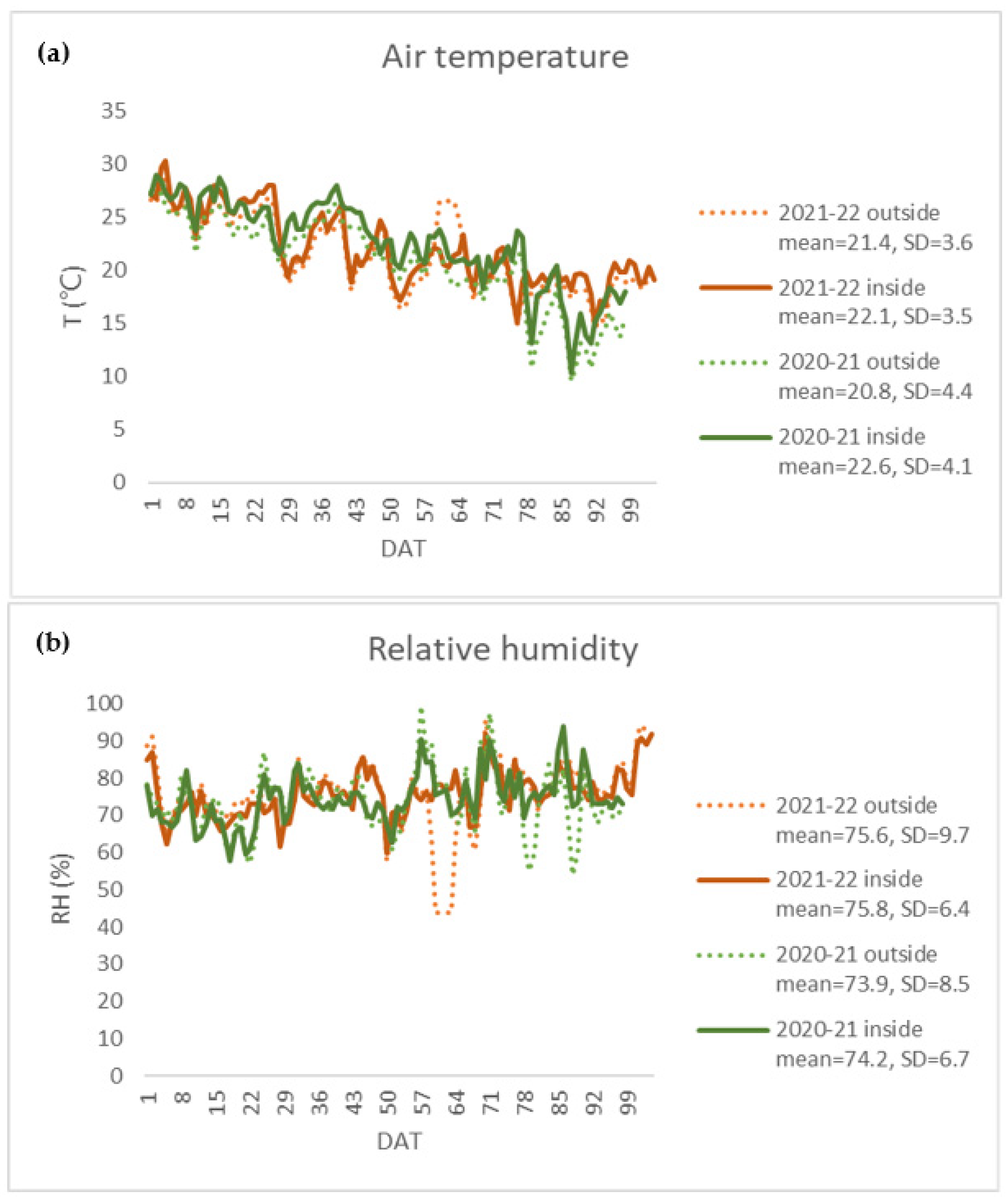
Figure 1 shows the daily mean air temperature and RH during the 2020–2021 and 2021–2022 crop seasons with no obvious difference in environmental conditions. Daily mean air temperature showed a decreasing trend in both crop seasons. The temperature variation outside the greenhouse was larger than those inside the greenhouse (SDinside SDoutside). The daily mean RH inside the greenhouse fluctuated around 60% and 90% throughout the crop seasons, while the daily mean RH outside the greenhouse varied from 45% to nearly 100%. Thus, the greenhouse environment was relatively stable compared with the open field.
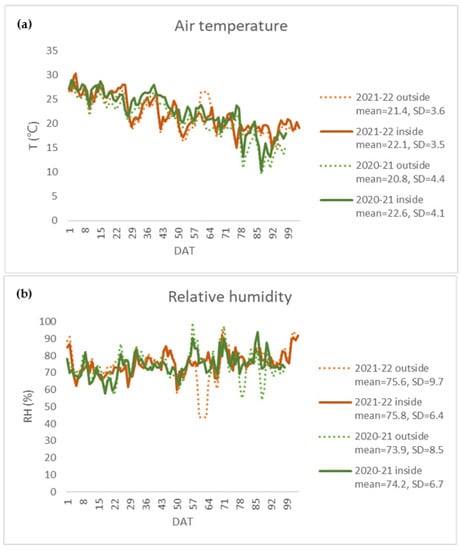
Figure 1.
Daily mean temperature (T, °C) (a) and relative humidity (RH, %) (b) inside and outside the greenhouse during the 2020–2021 and 2021–2022 crop seasons.
2.2. Establishment of the Sigmoid Growth Models
When establishing the growth model of the five traits of tomato, i.e., PH, LAI, SDM, LDM, and FDM, we considered two types of independent variables, DAT and GDD. TBASE of tomato was set as 10 °C when calculating GDD [26]. Before modeling, we produced the scatter plot of the dependent variable against each independent variable to confirm the suitability of fitting the growth model with a sigmoid curve. If the relationship between the independent and dependent variable was S-shaped, two sigmoid models, the Gompertz (Equation (1)) and Logistic (Equation (2)), were used to fit the data.
where a denotes the asymptotic value of the dependent variable, b is the location parameter related to the initial value of the model, c is the parameter that affects the growth rate in the curve, e is the base of the natural logarithm, and εi is the error term.
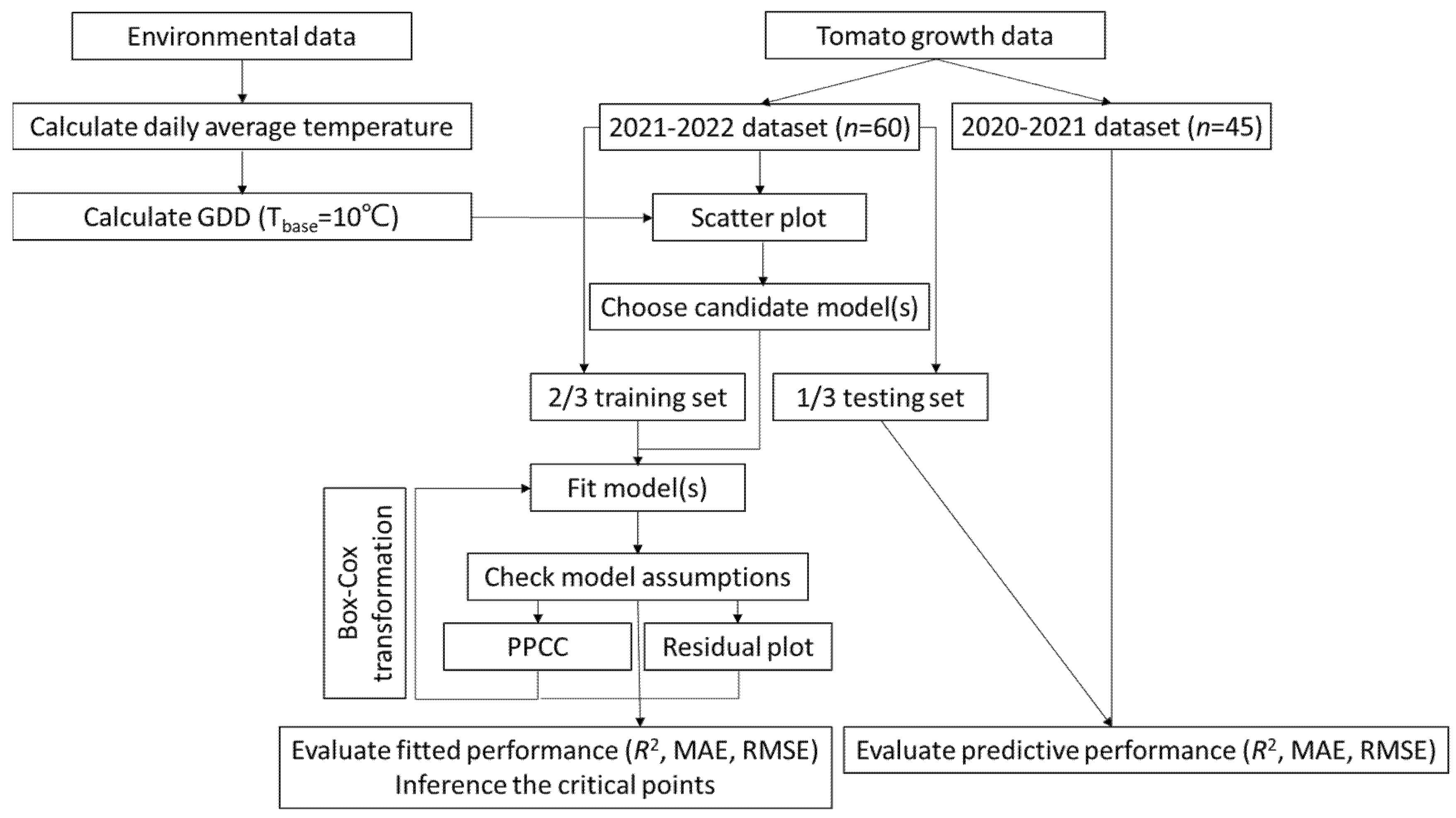
We randomly selected 2/3 of the 2021–2022 data for model calibration, and the remaining 1/3 of the data were used for model validation. Due to the small amount of data gathered during the 2020–2021 growth season, it was only used as another validation set. Before selecting a candidate model, the assumptions, such as those of normality and variance homogeneity, were examined. We used the probability plot correlation coefficient (PPCC), which is the correlation coefficient between the model residuals and their expected quantiles under a normal distribution, to test the normality hypothesis [32]. The higher the calculated PPCC, the better the model residuals follow a normal distribution. The assumption of homogeneity of variance was tested using residual plots of the model. An ideal residual plot should have residuals scattered randomly around 0 and not in a megaphone shape [33]. If the model violated the assumptions, the Box-Cox procedure (Equation (3)) was used to transform the data to make it follow the assumptions. The Box-Cox procedure can automatically identify a transformation from the family of power transformations on the dependent variable [33].
where is the dependent variable after transformation, Y is the untransformed dependent variable, and λ is a parameter determined from the data.
2.3. Model Performance Evaluation
Both the coefficient of determination (R2) (Equation (4)) and mean absolute error (MAE) (Equation (5)) were used to evaluate the model performance during the calibration and validation. For R2, larger values signify higher model performance. Contrarily, for MAE, the lower values indicate a better model. Additionally, the root mean square error (RMSE) (Equation (6)) was used to evaluate the goodness-of-fit of each model. For RMSE, the lowest values indicate the optimal model.
where SSE is the error sum of squares of the model, SST is the total sum of squares of the model, n is the number of observations, is the ith observation value, is the fitted value of the ith observation, and p is the number of parameters in the model. Both the Logistic and Gompertz models have three parameters (i.e., a, b, and c).
2.4. Critical Points of the Logistic and Gompertz Models
AAP and ADP can be calculated by equalizing the fourth derivative of the growth function to zero. MAP and MDP are found by equalizing the third derivative of the growth function to zero. IP is determined by equalizing the second derivative of the growth function to zero. Korkmaz et al. [31] already determined these critical points of the Logistic curve. In this paper, we only derived the Gompertz curve’s critical points; the derivation process can be found in the Appendix A. Here, we summarized the critical points of the two growth curves as Table 1.

Table 1.
Critical points of the Logistic and Gompertz models. a, b, and c are the estimated parameters of the two growth models, and e is the base of the natural logarithm.
2.5. Statistical Analysis
All statistical analyses were implemented using the R software (version 4.1.3; R Foundation for Statistical Computing, Vienna, Austria), with ‘minpack.lm’ (version 1.2-2) and ‘ppcc’ (version 1.2) packages used for model fitting and normality verification, respectively. For parameter estimation of nonlinear model, the ‘minpack.lm’ package was employed to obtain the numerical solution by minimizing residual sum of squares based on the Levenberg-Marquardt algorithm [34]. ‘EnvStats’ package (version 2.7.0) was used to conduct Box-Cox transformation when the model did not meet the assumptions.
3. Results and Discussion
In the present study, we employed Logistic and Gompertz models to connect the several growth traits (i.e., PH, LAI, SDM, LDM, and FDM) of tomatoes with DAT and cumulative GDD. To construct a model that exhibits good adaptability, a series of steps are required, including: (1) selecting suitable model types, (2) checking model assumptions, (3) fitting models, (4) evaluating model performance, and (5) model interpretation [1,35]. The overall research schema is summarized in Figure 2.

Figure 2.
Workflow of the model building and analysis in this study.
3.1. Verifying the Model Assumptions
Because the residuals of the fitted model (based on the original data) violated the assumptions of homogeneity of variance (Figures S2–S5), we implemented the Box-Cox procedure to transform the data. The λ values obtained are shown in Table 2. After the variable transformation, the PPCC values of the models were all higher than 0.87, indicating that the model residuals obeyed the normality assumption (Table S1). The residual plots revealed that the violations of assumptions were improved substantially after the data transformation (Figures S2–S5). However, even after the data transformation, there was still heteroscedasticity in the model residuals (Figures S2–S5). Meade et al. [36] and Thornley and France [37] considered that heteroscedasticity was common in the establishment of growth models since the increase in measurement was often accompanied by an increase in the overall variance.

Table 2.
λ values of the Box-Cox transformation.
3.2. Evaluation of the Fitted and Predictive Performance of the Models
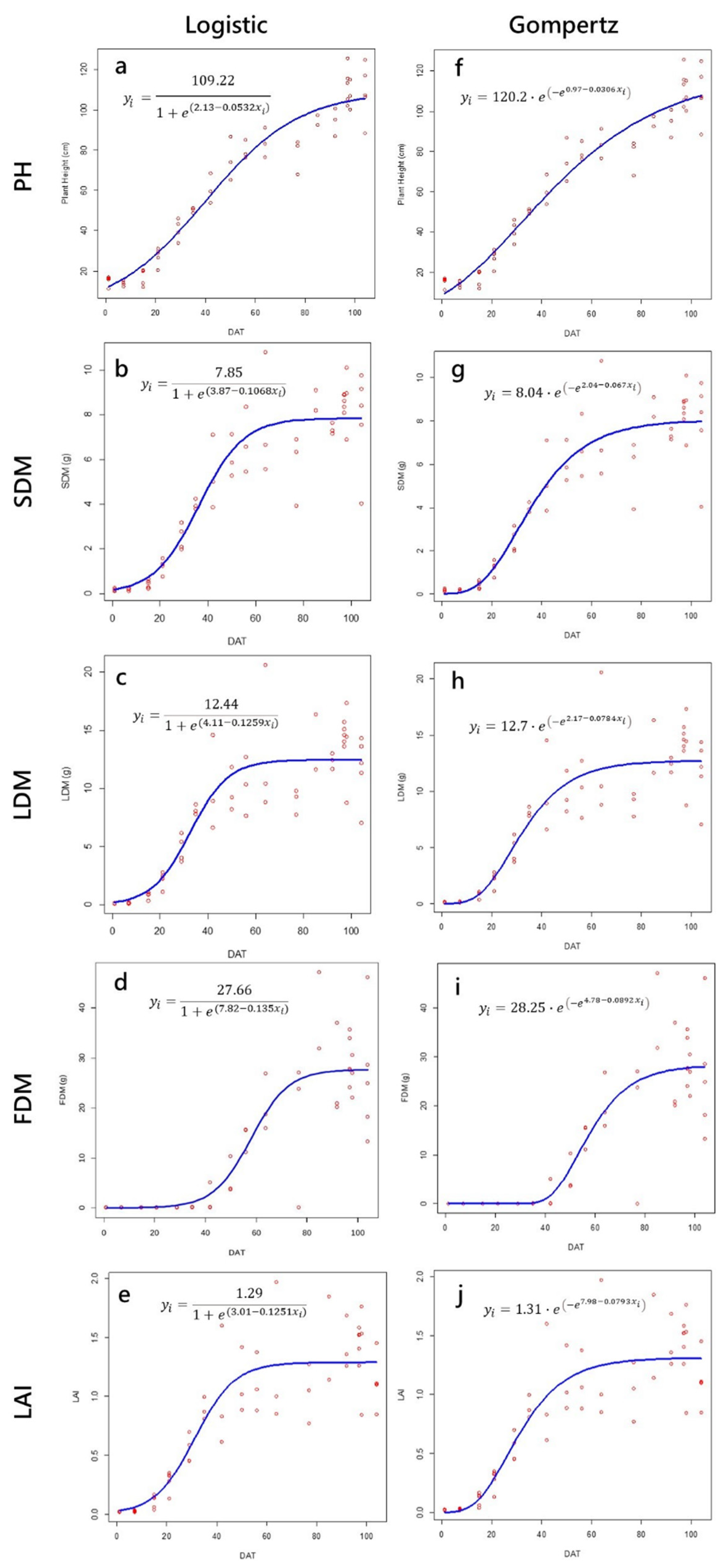
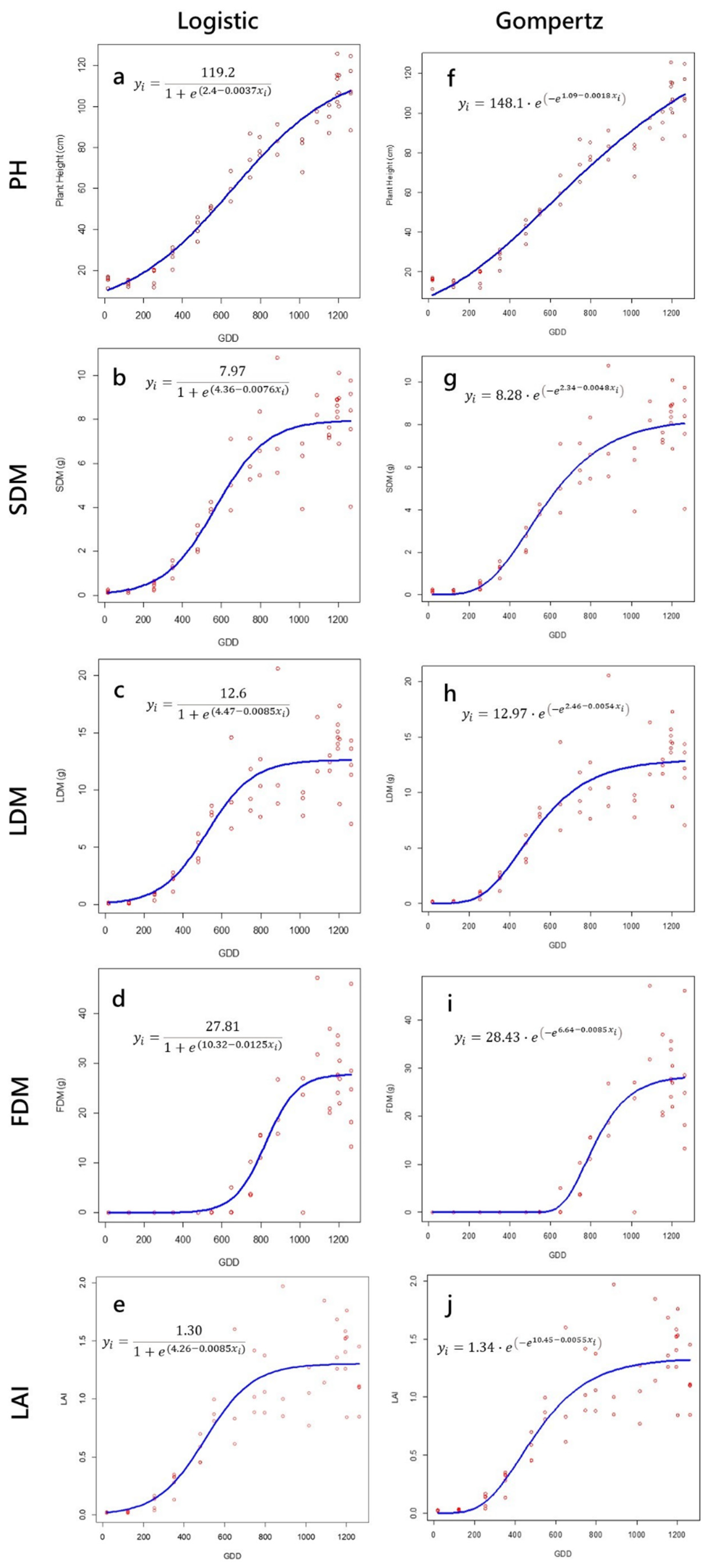
From the examination of the scatter plots of the observations of each trait against the DAT and GDD, the relationships of five traits (i.e., PH, LAI, SDM, LDM, and FDM) with DAT and GDD are all S-shaped (Figure 3 and Figure 4). The fitted Logistic and Gompertz growth curves can describe the relationship between variables well (Figure 3 and Figure 4). The R2 values of the models are between 0.82–0.97, and MAE values are low in calibration (Table 3). The R2 values using 1/3 of the data from the 2021–2022 season for validation are between 0.77–0.95 (Table 4), and those for the 2020–2021 season are between 0.64–0.92 (Table 5), indicating that these models can be used for prediction.
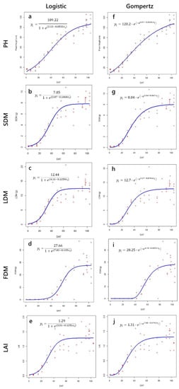
Figure 3.
Scatter plots of the observations and fitted Logistic (left column) and Gompertz (right column) growth curves with days after transplanting (DAT) as the independent variable. (a) Plant height, (b) stem dry matter, (c) leaves dry matter, (d) fruits dry matter, and (e) leaf area index of the Logistic model. (f) Plant height, (g) stem dry matter, (h) leaves dry matter, (i) fruits dry matter, and (j) leaf area index of the Gompertz model.
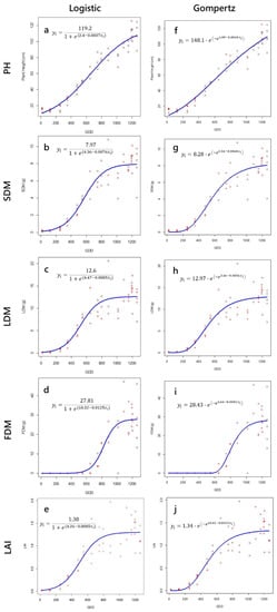
Figure 4.
Scatter plots of the observations and fitted Logistic (left column) and Gompertz (right column) growth curves with growing degree-days (GDD) as the independent variable. (a) Plant height, (b) stem dry matter, (c) leaves dry matter, (d) fruits dry matter, and (e) leaf area index of the Logistic model. (f) Plant height, (g) stem dry matter, (h) leaves dry matter, (i) fruits dry matter, and (j) leaf area index of the Gompertz model.

Table 3.
Calibration results of the sigmoid growth models established with the 2/3 of the 2021–2022 crop season data.

Table 4.
Validation of the sigmoid growth models established in 2021–2022 using the 1/3 of 2021–2022 crop season data.

Table 5.
Validation of the sigmoid growth models established in 2021–2022 using the 2020–2021 crop season data.
For each trait, the Logistic and Gompertz curves have similar performances at R2, MAE, and RMSE (Table 3, Table 4 and Table 5). Although the two models are sigmoid curves, their growth trends are different. That is, the Logistic curve is symmetric, whereas the Gompertz curve is asymmetric [36,38]. It means that the height (Y coordinate) of the IP for the Logistic curve is exactly half the entire curve. On the other hand, the height of the IP of the Gompertz curve is smaller than that of the Logistic function. The symmetric characteristic may be a limitation for some growth processes, which cannot meet the characteristic of the Logistic function [36,39]. The Gompertz function may also meet the features of some growth processes better than that of the Logistic function [36,39]; however, the performance of the Logistic model is comparable to or better than that of the Gompertz model [1,39]. These findings are consistent with our results. Figure 3 and Figure 4 showed that the growth of the Logistic curve was slow at the initial stage, and dropped rapidly in later stages; however, the growth of the Gompertz curve was very fast at the beginning and decreases slowly in the later stages. Therefore, if resources permit, both Logistic and Gompertz functions should be considered, which is in agreement with Vieira and Hoffmann [39].
In the comparison of two types of independent variables, the model with GDD as the independent variable performs slightly better than the model with DAT as the independent variable (Table 3, Table 4 and Table 5) because GDD takes additional temperature-related information into account than DAT. The performance of models did not show much difference in whether the GDD or DAT was used as an independent variable, the reason may be that there was no significant difference in environmental conditions between the two seasons (Figure 1). However, because the climate usually changes, the use of GDD may predict crop growth more accurately than DAT [40,41].
Comparing the model of different traits, the prediction performance of LAI is relatively poor compared to other traits (Table 3, Table 4 and Table 5). This result is consistent with previous studies where the simulation of LAI was difficult and with low accuracy [5,26]. However, our performance of the sigmoid curve simulation of LAI is still acceptable (R2 0.70, MAE 0.25, RMSE 1.18) (Table 3, Table 4 and Table 5). In addition, the predictive performance of 2020–2021 is worse than that of 2021–2022, especially for PH (Table 4 and Table 5). We probably did not consider other important factors that may affect the growth of tomatoes such as light. Temperature and solar radiation are the most important climate factors affecting crop growth [5,21,42]. However, the change in temperature inside the greenhouse does not follow the pattern of solar radiation as closely as in the open field, thus using GDD alone may not be enough to accurately predict crop growth inside greenhouses [5,21]. Therefore, to control error variation more effectively and improve the predictive ability of the model, additional light-related variables should be considered.
3.3. Inferences in Critical Points
One of the advantages of using sigmoid curves to build growth models is that some biologically meaningful parameters can be derived from the mathematical properties of the curve [31], which can be coordinated with agricultural practices [24,25,43]. Silva et al. [44] used the critical points of growth models to observe the harvest time of ‘Green Dwarf’ coconut fruits with the best water flavor. Diel et al. [45] characterized the production of biquinho pepper by the interpretation of Logistic model’s parameters and critical points, and discovered the best cultivar and growing season for subtropical region. The critical points of DAT and GDD derived from the two curves for each trait are shown in Table 6 and Table 7, respectively. The AAP, MAP, and IP of the Logistic model are all later than those estimated by the Gompertz model; the interval between MDP and ADP of the Logistic model is shorter than that of the Gompertz model (Table 6 and Table 7). These characteristics reflect the different properties of the two sigmoid curves. The Gompertz model is a fast-growing curve in the early stage, while the Logistic is a rapidly stable curve in the later stages. Overall, the critical points estimated by the Logistic model are closer to our expectation than those of the Gompertz model.

Table 6.
Critical days after transplanting.

Table 7.
Critical growing degree-days.
Because APP is known as a lag time point [31], there is almost no crop growth before the APP, which also reflects the time required for tomatoes to adapt to the new environment and rebuild their roots after transplanting. From Table 6 and Table 7, the PH is the earliest growth trait, and most of the AAP values of PH are negative, indicating that PH has started to grow before transplanting. SDM and LDM reach AAP almost simultaneously but the subsequent LDM grows faster than SDM (Table 6 and Table 7). In addition, the critical points of LAI are approximately 1–2 days earlier than that of LDM, revealing that young tissues have higher water content (Table 6). The IP determines the time at which the growth rate is maximum. According to the results of the Logistic model, the growth rate of tomato stems and leaves reaches a peak approximately one month after transplanting (Table 6) when the GDD is 525–575 °C (Table 7). The growth rate of tomato fruit reaches its peak approximately two months after transplanting (Table 6) when the GDD is approximately 825 °C (Table 7). If the crop requires any growth management such as fertilization, it is most efficient before the IP [24,43]. In general, when the IP can be reached in a smaller GDD or DAT, it indicates that the growth under this situation is more precocious [46]. A short interval between MAP and MDP showed that the production was concentrated in a short time [46]. Finally, at the ADP, plant growth tends to stabilize towards the end of its production cycle. After ADP, too much nutrition will not significantly promote the growth of crops, while the fertilizer input should be carefully controlled.
Both the Logistic and Gompertz models need only three parameters (i.e., a, b, and c) to describe the growth of tomatoes, producing acceptable and interpretable results [1,47,48]. However, it is worth noting that the Logistic and Gompertz models are both empirical models, so the conclusions that can be drawn from the experiment will depend on the manner in which the data were collected [49]. Therefore, the reliability of empirical models needs to be validated using the experimental data of more varieties and a wider range of climate conditions. Nonetheless, because the greenhouse environment can be regulated and is relatively stable compared with the open field, the growth of crops can be efficiently predicted by the experimentally determined models. Shi et al. [50] evaluated the performance of a novel beta sigmoid function using real and simulated the DM data of six crop species generated by four commonly used growth functions (i.e., the exponential, Logistic, Gompertz, and von Bertalanffy equations). Compared to other growth models, the beta sigmoid function allowed for both symmetric and asymmetric growth, and it performed better than the above growth functions. Kocian et al. [51] proposed a Bayesian machine learning approach to dynamically model the sigmoid-type growth of greenhouse crops. It was found that this approach could accurately fit the data, and it was more robust to the changes of different environmental conditions. In the future, we can use novel growth models or combine machine learning methods to further enhance the model performance and the robustness to the environmental change.
4. Conclusions
In the present study, we collected tomato growth data for two crop seasons in Taiwan and established growth models using two sigmoid functions (i.e., the Gompertz and Logistic curves). The growth models established in this study can accurately predict the growth of five important traits of tomato, including PH, LAI, SDM, LDM, and FDM. In addition, we inferred five critical points that can be used for practical management based on the proposed growth models. The performances of GDD models were slightly better than those of the DAT models. Although there was no significant difference in model performance between the Gompertz and Logistic models, the critical points estimated by the Logistic model are closer to our expectation than those of the Gompertz model. Therefore, the Logistic model developed in this study is more applicable for greenhouse ‘993′ tomatoes compared to the Gompertz model. When these models are used to predict the growth of tomatoes, the GDD predictions using local weather forecasts or historical weather data can be used to adjust the planned fieldwork schedule based on the traditional calendar day method. Since the greenhouse environment is relatively stable and can be controlled, the empirical model has several potential applications. Finally, the reliability of the model can be improved using experimental data of more varieties and climatic conditions.
Supplementary Materials
The following supporting information can be downloaded at: https://www.mdpi.com/article/10.3390/horticulturae8111021/s1, Table S1: Probability plot correlation coefficient (PPCC) of sigmoid growth model established with DAT and GDD as independent variables and PH, SDM, LDM, FDM, and LAI as dependent variables; Figure S1: The research site map of this study; Figure S2: Residual plots before (left column) and after (right column) data transformation of the Gompertz curve with days after transplanting (DAT) as the independent variable; Figure S3: Residual plots before (left column) and after (right column) data transformation of the Logistic curve with days after transplanting (DAT) as the independent variable; Figure S4: Residual plots before (left column) and after (right column) data transformation of Gompertz curve with growing degree-days (GDD) as the independent variable; Figure S5: Residual plots before (left column) and after (right column) data transformation of the Logistic curve with growing degree-days (GDD) as the independent variable.
Author Contributions
Conceptualization, B.-J.K. and S.-L.F.; Data curation, S.-L.F., Y.-H.K., L.K. and C.-C.C.; Formal analysis, S.-L.F. and Y.-H.K.; Funding acquisition, M.-H.Y. and B.-J.K.; Investigation, S.-L.F., Y.-H.K., L.K. and C.-C.C.; Methodology, S.-L.F., Y.-H.K. and C.-Y.H.; Writing–original draft, S.-L.F. and Y.-H.K.; Writing–review & editing, B.-J.K. All authors have read and agreed to the published version of the manuscript.
Funding
This work was financially supported by the “Innovation and Development Center of Sustainable Agriculture” from the Featured Areas Research Center Program within the framework of the Higher Education Sprout Project by the Ministry of Education (MOE) in Taiwan. This research was also supported (in part) by the Smart Sustainable New Agriculture Research Center (SMARTer) project (NSTC 110-2634-F-005-006).
Data Availability Statement
Not applicable.
Conflicts of Interest
The authors declare no conflict of interest.
Appendix A
The points (,), (,), (,), (,), and (,) correspond to IP, MAP, MDP, AAP, and ADP of the Gompertz model, respectively.
References
- Hsieh, C.-Y.; Fang, S.-L.; Wu, Y.-F.; Chu, Y.-C.; Kuo, B.-J. Using sigmoid growth curves to establish growth models of tomato and eggplant stems suitable for grafting in subtropical countries. Horticulturae 2021, 7, 537. [Google Scholar] [CrossRef]
- Streck, N.; Bosco, L.C.; Lucas, D.D.P.; Lago, I. Modelagem da emissão de folhas em arrozvermelho. Pesqui. Agropecu. Bras. 2008, 43, 559–567. [Google Scholar] [CrossRef]
- Acock, B.; Reynolds, J.F. The rationale for adopting a modular generic structure for crop simulators. Acta Hortic. 1989, 248, 391–400. [Google Scholar] [CrossRef]
- Challa, H. Report of the working party on crop growth models. Acta Hortic. 1985, 174, 169–176. [Google Scholar] [CrossRef]
- Marcelis, L.F.M.; Heuvelink, E.; Goudriaan, J. Modelling biomass production and yield of horticultural crops: A review. Sci. Hortic. 1998, 74, 83–111. [Google Scholar] [CrossRef]
- Hou, P.; Liu, Y.; Xie, R.; Ming, B.; Ma, D.; Li, S.; Mei, X. Temporal and spatial variation in accumulated temperature requirements of maize. Field Crop. Res. 2014, 158, 55–64. [Google Scholar] [CrossRef]
- Liu, Y.; Su, L.; Wang, Q.; Zhang, J.; Shan, Y.; Deng, M. Comprehensive and quantitative analysis of growth characteristics of winter wheat in China based on growing degree days. Adv. Agron. 2020, 159, 237–273. [Google Scholar] [CrossRef]
- Perry, K.B.; Wu, Y.; Sanders, D.C.; Garrett, J.T.; Decoteau, D.R.; Nagata, R.T.; Dufault, R.J.; Batal, K.D.; Granberry, D.M.; Mclaurin, W.J. Heat units to predict tomato harvest in the southeast USA. Agric. Forest Meteorol. 1997, 84, 249–254. [Google Scholar] [CrossRef][Green Version]
- Gramig, G.G.; Stoltenberg, D.E. Leaf appearance base temperature and phyllochron for common grass and broadleaf weed species. Weed Technol. 2007, 21, 249–254. [Google Scholar] [CrossRef]
- McMaster, G.S.; Wilhelm, W.W. Growing degree-days: One equation, two interpretations. Agric. For. Meteorol. 1997, 87, 291–300. [Google Scholar] [CrossRef]
- Wannasek, L.; Ortner, M.; Amon, B.; Amon, T. Sorghum, a sustainable feedstock for biogas production? Impact of climate, variety and harvesting time on maturity and biomass yield. Biomass Bioenerg. 2017, 106, 137–145. [Google Scholar] [CrossRef]
- Narayanan, S.; Aiken, R.M.; Prasad, P.V.; Xin, Z.; Paul, G.; Yu, J. A simple quantitative model to predict leaf area index in sorghum. Agron. J. 2014, 106, 219–226. [Google Scholar] [CrossRef]
- Tripathi, A.M.; Pohanková, E.; Fischer, M.; Orság, M.; Trnka, M.; Klem, K.; Marek, M.V. The evaluation of radiation use efficiency and leaf area index development for the estimation of biomass accumulation in short rotation poplar and annual field crops. Forests 2018, 9, 168. [Google Scholar] [CrossRef]
- Medrano, E.; Lorenzo, P.; Sánchez-Guerrero, M.C.; Montero, J.I. Evaluation and modelling of greenhouse cucumber crop transpiration under high and low radiation conditions. Sci. Hortic. 2005, 105, 163–175. [Google Scholar] [CrossRef]
- Ta, T.H.; Shin, J.H.; Ahn, T.I.; Son, J.E. Modeling of transpiration of paprika (Capsicum annuum L.) plants based on radiation and leaf area index in soilless culture. Hortic. Environ. Biotechnol. 2011, 52, 265–269. [Google Scholar] [CrossRef]
- Carmassi, G.; Bacci, L.; Bronzini, M.; Incrocci, L.; Maggini, R.; Bellocchini, G.; Massa, D.; Pardossi, A. Modelling transpiration of greenhouse gerbera (Gerbera jamesonii H. Bolus) grown in substrate with saline water in a Mediterranean climate. Sci. Hortic. 2013, 156, 9–18. [Google Scholar] [CrossRef]
- Chin, D.A.; Fan, X.H.; Li, Y.C. Validation of growth and nutrient uptake models for tomato on a gravelly South Florida soil under greenhouse conditions. Pedosphere 2011, 21, 46–55. [Google Scholar] [CrossRef]
- Massa, D.; Incrocci, L.; Maggini, R.; Bibbiani, C.; Carmassi, G.; Malorgio, F.; Pardossi, A. Simulation of crop water and mineral relations in greenhouse soilless culture. Environ. Model. Softw. 2011, 26, 711–722. [Google Scholar] [CrossRef]
- Medrano, E.; Alonso, F.J.; Sanchez-Guerrero, M.C.; Lorenzo, P. Incorporation of a model to predict crop transpiration in a commercial irrigation equipment as a control method for water supply to soilless horticultural crops. Acta Hortic. 2008, 801, 1325–1330. [Google Scholar] [CrossRef]
- Xu, R.; Dai, J.; Luo, W.; Yin, X.; Li, Y.; Tai, X.; Han, L.; Chen, Y.; Lin, L.; Li, G.; et al. A photothermal model of leaf area index for greenhouse crops. Agric. For. Meteorol. 2010, 150, 541–552. [Google Scholar] [CrossRef]
- Dai, J.; Luo, W.; Li, Y.; Yuan, C.; Chen, Y.; Ni, J. A simple model for prediction of biomass production and yield of three greenhouse crops. Acta Hort. 2006, 718, 81–88. [Google Scholar] [CrossRef]
- Gong, X.; Qiu, R.; Sun, J.; Ge, J.; Li, Y.; Wang, S. Evapotranspiration and crop coefficient of tomato grown in a solar greenhouse under full and deficit irrigation. Agric. Water Manag. 2020, 235, 106154. [Google Scholar] [CrossRef]
- Confalonieri, R.; Bregaglio, S.; Rosenmund, A.S.; Acutis, M.; Savin, I. A model for simulating the height of rice plants. Eur. J. Agron. 2011, 34, 20–25. [Google Scholar] [CrossRef]
- Bem, C.M.; Cargnelutti Filho, A.; Chaves, G.G.; Kleinpaul, J.A.; Lavezo, A. Gompertz and Logistic models to the productive traits of sunn hemp. J. Agric. Sci. 2018, 10, 225–238. [Google Scholar] [CrossRef]
- Bem, C.M.; Cargnelutti Filho, A.; Facco, G.; Schabarum, D.E.; Silveira, D.L.; Simões, F.M.; Uliana, D.B. Growth models for morphological traits of sunn hemp. Semin. Cienc. Agrar. 2017, 38, 2933–2944. [Google Scholar] [CrossRef]
- Gallardo, M.; Fernández, M.D.; Giménez, C.; Padilla, F.M.; Thompson, R.B. Revised VegSyst model to calculate dry matter production, critical N uptake and ETc of several vegetable species grown in Mediterranean greenhouses. Agric. Syst. 2016, 146, 30–43. [Google Scholar] [CrossRef]
- Jiang, T.; Liu, J.; Gao, Y.; Sun, Z.; Chen, S.; Yao, N.; Ma, H.; Feng, H.; Yu, Q.; He, J. Simulation of plant height of winter wheat under soil water stress using modified growth functions. Agric. Water Manag. 2020, 232, 106066. [Google Scholar] [CrossRef]
- Singh, S.K.; Verma, C.L.; Sharma, D.K. Plant height model for eucalyptus plantations for biodrainage use. Int. J. Eng. Res. Technol. 2014, 3, 250–259. [Google Scholar]
- Cao, L.; Shi, P.J.; Li, L.; Chen, G. A new flexible sigmoidal growth model. Symmetry 2019, 11, 204. [Google Scholar] [CrossRef]
- Zeide, B. Analysis of growth equations. For. Sci. 1993, 39, 594–616. [Google Scholar] [CrossRef]
- Korkmaz, M.; Oda, V.; Basustaoglu, E.O. A study over determination of asymptotic deceleration and absolute acceleration points in logistic growth model. Turk. J. Math. Comput. Sci. 2018, 10, 33–37. [Google Scholar]
- Filliben, J.J. The probability plot correlation coefficient test for normality. Technometrics 1975, 17, 111–117. [Google Scholar] [CrossRef]
- Kutner, M.H.; Nachtsheim, C.J.; Neter, J.; Li, W. Applied Linear Statistical Models, 5th ed.; McGraw-Hill: New York, NY, USA, 2004. [Google Scholar]
- Elzhov, T.V.; Mullen, K.M.; Spiess, A.-N.; Bolker, B.; Mullen, M.K.M.; Suggests, M. Package ‘minpack.lm.’ Title R Interface Levenberg-Marquardt Nonlinear Least-Sq. Algorithm Found MINPACK Plus Support Bounds’. 2016. Available online: https://cran.r-project.org/web/packages/minpack.lm/minpack.lm.pdf (accessed on 22 October 2022).
- Archontoulis, S.A.; Miguez, F.E. Nonlinear regression models and applications in agricultural research. Agron. J. 2015, 107, 786–798. [Google Scholar] [CrossRef]
- Meade, K.A.; Cooper, M.; Beavis, W.D. Modeling biomass accumulation in maize kernels. Field Crops Res. 2013, 151, 92–100. [Google Scholar] [CrossRef]
- Thornley, J.H.M.; France, J. Mathematical Models in Agriculture: Quantitative Methods for the Plant, Animal and Ecological Sciences, 2nd ed.; CAB International: Wallingford, UK, 2007. [Google Scholar]
- Franses, P.H. A method to select between Gompertz and logistic trend curves. Technol. Forecast. Soc. Chang. 1994, 46, 45–49. [Google Scholar] [CrossRef]
- Vieira, S.; Hoffmann, R. Comparison of the logistic and the Gompertz growth functions considering additive and multiplicative error terms. Appl. Statist. 1977, 26, 143–148. [Google Scholar] [CrossRef]
- Bonhomme, R. Bases and limits to using ‘degree.day’ units. Eur. J. Agron. 2000, 13, 1–10. [Google Scholar] [CrossRef]
- Liu, L.W.; Lu, C.T.; Wang, Y.M.; Lin, K.H.; Ma, X.; Lin, W.S. Rice (Oryza sativa L.) growth modeling based on growth degree day (GDD) and artificial intelligence algorithms. Agriculture 2022, 12, 59. [Google Scholar] [CrossRef]
- Doan, C.C.; Tanaka, M. Relationships between tomato cluster growth indices and cumulative environmental factors during greenhouse cultivation. Sci. Hortic. 2022, 295, 110803. [Google Scholar] [CrossRef]
- Bem, C.M.; Cargnelutti Filho, A.; Carini, F.; Pezzini, R.V. Univariate and multivariate nonlinear models in productive traits of the sunn hemp. Rev. Ciên. Agron. 2020, 51, e20196673. [Google Scholar] [CrossRef]
- Silva, É.M.; Fruhauf, A.C.; Silva, E.M.; Muniz, J.A.; Fernandes, T.J.; Silva, V.F. Evaluation of the critical points of the most adequate nonlinear model in adjusting growth data of ‘green dwarf’ coconut fruits. Rev. Bras. Frutic. 2021, 43, e726. [Google Scholar] [CrossRef]
- Diel, M.I.; Lúcio, A.D.; Valera, O.V.S.; Sari, B.G.; Olivoto, T.; Pinheiro, M.V.M.; Melo, P.J.; Tartaglia, F.L.; Schmidt, D. Production of biquinho pepper in different growing seasons characterized by the logistic model and its critical points. Ciênc. Rural 2020, 50, e20190477. [Google Scholar] [CrossRef]
- Sari, B.G.; Olivoto, T.; Diel, M.I.; Krysczun, D.K.; Lúcio, A.D.; Savian, T.V. Nonlinear modeling for analyzing data from multiple harvest crops. Agron. J. 2018, 110, 2331–2342. [Google Scholar] [CrossRef]
- Sari, B.G.; Lúcio, A.D.C.; Santana, C.S.; Olivoto, T.; Diel, M.I.; Krysczun, D.K. Nonlinear growth models: An alternative to ANOVA in tomato trials evaluation. Eur. J. Agron. 2019, 104, 21–36. [Google Scholar] [CrossRef]
- Sari, B.G.; Lúcio, A.D.C.; Santana, C.S.; Savian, T.V. Describing tomato plant production using growth models. Sci. Hortic. 2019, 246, 146–154. [Google Scholar] [CrossRef]
- Whisler, F.D.; Acock, B.; Baker, D.N.; Fye, R.E.; Hodges, H.F.; Lambert, J.R.; Lemmon, H.E.; McKinion, J.M.; Reddy, V.R. Crop simulation models in agronomic systems. Adv. Agron. 1986, 40, 141–208. [Google Scholar] [CrossRef]
- Shi, P.J.; Chen, L.; Hui, C.; Grissino-Mayer, H.D. Capture the time when plants reach their maximum body size by using the beta sigmoid growth equation. Ecol. Modell. 2016, 320, 177–181. [Google Scholar] [CrossRef]
- Kocian, A.; Carmassi, G.; Cela, F.; Incrocci, L.; Milazzo, P.; Chessa, S. Bayesian sigmoid-type time series forecasting with missing data for greenhouse crops. Sensors 2020, 20, 3246. [Google Scholar] [CrossRef]
Publisher’s Note: MDPI stays neutral with regard to jurisdictional claims in published maps and institutional affiliations. |
© 2022 by the authors. Licensee MDPI, Basel, Switzerland. This article is an open access article distributed under the terms and conditions of the Creative Commons Attribution (CC BY) license (https://creativecommons.org/licenses/by/4.0/).

