Prediction Models for the Plant Coverage Percentage of a Vertical Green Wall System: Regression Models and Artificial Neural Network Models

Abstract

(1) Background: The expansion that most cities have been showing for more than half a century has also brought with it an increase in the density of buildings, most of the time at the expense of green areas. This has led to negative effects, such as overpopulation of cities, rising urban temperatures, pollution of water, air, soil, and others, affecting daily urban life. As a result, specialists from different fields form multidisciplinary teams are looking for solutions to counteract these effects. The subject of visible facades has registered an increased interest among researchers in recent years because they can represent a viable solution that can contribute to increasing the degree of urban comfort. However, for such a system to be effective, it is necessary that the plants used grow and develop harmoniously and ensure the best possible coverage of the facade. The aim of this research is to find an adequate mathematical model that can predict, with a high degree of accuracy, the percentage of plant coverage of a green wall system, which is positioned in the city of Iasi, northeastern Romania. (2) Methods: The models used for this purpose were a multiple linear regression model (MLR) and a model based on a feed-forward artificial neural network (ANN). Four independent variables (soil temperature, soil moisture, week of the year, and cardinal wall orientation) and the interaction between two variables (soil temperature and week of the year) were used for the multiple linear regression model. Artificial neural networks were also trained to estimate the percentage of plant coverage in the analyzed system, and the network with the best mean squared error performance was chosen in doing predictions. For both MLR and ANN models, we constructed confidence intervals for the degree of plant coverage of the system (PCP) for a set of observed values. In the case of the ANN model, the confidence interval was derived via the bootstrap method, which is a resampling with replacement technique used to generate new samples from the original dataset. To the best of our knowledge, the derivation of confidence intervals using a combination of neural networks with the bootstrap method has not been used before, at least for predictions in horticulture. (3) Results: The ANN employed here consisted of one input layer with four neurons, one hidden layer with five neurons, and one output layer with one neuron. The comparison showed that the confidence interval obtained using ANN has a shorter length (and thus it is more accurate) than that obtained by the multiple linear regression model. The choice of the experimental module façade had a significant influence (of magnitude 1.9073) on the plant coverage percentage. An increase of one unit in soil humidity will determine an increase of almost 5.1% in plant coverage percentage, and an increase of 1 °C in soil temperature will determine a decrease of almost 1.21% in plant coverage percentage. The choice of the experimental module façade had a significant influence (of magnitude 1.9073) on the plant coverage percentage. (4) Conclusions: Although both methods showed to be useful in making predictions, the ANN method showed better predictive capabilities, at least when the performance is measured by the mean squared error. This fact may be useful when predicting the percentage of plant coverage of a green wall system with a higher degree of accuracy, in the case of organizing outdoor exhibitions or other similar projects.

1. Introduction

Urban development has led to an increase in the density of buildings to the detriment of green areas [1] which plays an important role in counteracting the negative effects of increased pollution [2,3,4]. Overcrowding, resource depletion, pollution, and health degradation are some of the environmental problems caused by excessive urbanization [5,6]. Simultaneously, the decrease in green areas on the perimeter of cities is a major factor in increasing urban heat, which further leads to an increase in energy consumption and air pollution, producing negative effects on health [6]. The benefits of green spaces in cities have become increasingly important because of the growing number of people who work, live, and spend their free time there. Depending on the location and occupied area, urban green areas have a beneficial influence on the climate, reduce pollution, and have aesthetic functions [7]. They also support local ecosystems and provide a place for social activities and psychological restoration, thus protecting the health of urban residents [8,9].

Therefore, the reintroduction of green areas in urban areas can reduce some of the negative consequences of urbanization [8,9,10,11]. However, due to the limited space of free construction land that could be developed for this purpose, other less conventional surfaces were sought for their establishment. As a result, building roofs and facades have become attractive as supporting surfaces for the creation of green areas, thus increasing the greening of cities [7]. A key design aspect in the development of modern buildings to improve the quality of the environment is the use of plants not only for aesthetic purposes, but also to mitigate the effect produced by the urban heat island. Green walls also offer aesthetic variations in an environment in which people carry out their daily activities, and numerous studies have linked the presence of plants to improve human physical and mental health [12,13]. For their growth and development, plants absorb a significant amount of solar radiation, while also functioning as a solar barrier that prevents the absorption of solar radiation on a large scale. Their use is essential and can significantly improve the built environment [14].

Research has also confirmed that green roofs, walls, and facades can be valuable for the energy performance of buildings and for the mitigation of the urban microclimate [15,16,17]. They reduce the temperature peaks of the exterior surfaces of buildings during the summer [18,19,20,21]. The shading effect of the foliage and evapotranspiration processes significantly lowered the surface temperature. The additional effects of thermal resistance, shading, and evapotranspiration work together, and their specific effects are coupled and difficult to separate. Evapotranspiration affects the water content of the substrate and, consequently, the thermophysical properties of the plant component. Simultaneously, a higher density of foliage implies more plant perspiration and less soil evaporation [17].

The way people perceive green façades has been analyzed through surveys and questionnaires in European countries, such as the Netherlands, Slovenia [22], and Greece [23]. The impact of green facades on the perception of the urban environment suggests that green infrastructure plays a vital role in the perception of spatial users [22,23].

In order to be efficient in creating green walls, an evaluation of their implementation possibilities and the identification of possible locations that need green infrastructure is necessary. An example of good practice in this regard took place in Ljubljana (Slovenia), a city facing a variety of challenges related to economic transition and demographic changes [24].

For a green wall to offer maximum benefits, it is necessary to consider three factors that can influence its performance: the environment, the green wall system, and selected plant species. Environmental factors (climate and season) determine the intensity of solar radiation, precipitation, humidity, and wind speed, which play a role in supporting the evapotranspiration process of plants that transform water from the substrate into water vapor and release it into the air [25]. Therefore, it is necessary to carry out studies to identify decorative plant species that are planted in various vertical systems for green façades, reaching their maximum decorative potential under specific local climatic conditions.

An ANN is a complex neural network comprising a large group of simple neural cells that can be used to analyze several variables simultaneously. This type of network is used for forecasting and comparisons in several fields of research, such as river flood forecasting [26], monsoon precipitation forecasting in the Yangtze Delta [27], predicting the amount and concentration of substances that pollute the air in Seoul [28], and predicting the values of meteorological variables at the Turkish Meteorological Center [29]. In 2019, Runge and Zmereanu used an ANN to calculate advanced energy consumption and gas emissions in residential buildings, which is important for energy planning, optimization, and conservation [30]. In the field of floriculture, Lukas and his coworkers used several modeling methods to evaluate grassland plant coverage on the Tibetan Plateau [31].

Artificial neural networks and multi-linear regression modeling have become important research methods in horticulture. In a study carried out in 2019, these mathematical models were used to effectively predict acidity and sugar in fresh citrus fruits, where based on statistical criteria, the ANN developed in this study recorded better results than the MLR model in predicting the chemical attributes of fresh citrus fruits [32]. Artificial neural networks and multiple linear regression were used as the main methods for modeling the seed yield of safflower (Carthamus tinctorius L.). Thus, modeling the connections between safflower seed yield and its components is useful to understand the most important traits with significant effects on seed yield, which would help saffron growers in the selection of high-performance varieties [33]. Artificial neural networks have also been developed for the prediction of chemical attributes of fresh peach fruits [34], as well as for the optimization of peach fruit quality [35]. The MLR multiple linear regression technique was successfully used to predict the quality attributes of seedless grape bunches, as well as to evaluate the physical characteristics of the bunch and the color characteristics of Flame seedless grape berries [36].

In biology, Brion used ANN to analyze microbial water quality [37], and Li et al. made predictions for water quality using an ANN [38]. Madhiarasan conducted an analysis of artificial neural network performance based on factors influencing temperature forecasting applications [39].

Usually, the most convenient way to describe relationships among data is using linear regression methods, as we obtain a closed-form equation of the model, and the model parameters are easy to interpret. However, these methods can be applied only if a set of specific modeling assumptions are verified, and even so, they may fail to describe more complex dependencies between variables. Artificial neural networks have been around for quite a while, and they turned out to be very successful in classification and prediction problems. They can be trained to depict very complex nonlinear relationships in the data. ANNs use training data to develop their own representation for the analyzed parameters, and they do not need a priori modeling assumptions. They can dynamically select the best regression model, be it linear or multi-linear, logistic, exponential, etc. When the predictions made by an ANN are not as accurate as desired, they have an entire arsenal of hidden layers, which can be used to boost the prediction power with higher accuracy than a linear regression.

In this work, we built prediction models for the plant coverage percentage (PCP) of the experimental module based on the humidity in the soil on the experimental module faces, the temperature of the soil, the time of the year variable, and the orientation of the experimental module facade (N, E, S, W). We do this by examining two models: a multiple linear regression model and an artificial neural network approach. For both MLR and ANN models, we make predictions through confidence intervals for the degree of plant coverage of the system for a set of observed values, with the aim of comparison between them. In the case of the ANN model, the predictions were based on the bootstrap method [40]. For the computer implementation of the ANN, we have employed MATLAB software v9.8.0 (R2020a) with the neural network toolbox.

As explained in the following sections, the explanatory variables were carefully chosen from a set of possible predictors, though a correlation analysis, and the model with the best performance (in terms of MSE, R², adjusted R², utility of the model) was chosen. The multiple linear regression model contains an interaction term, representing the effect that the combinations of temperature and week of the year have on the degree of plant cover (PCP).

Despite the fact that there are many studies in the field of landscaping in recent years, to the best of our knowledge, there is still no study focused on the use of artificial neural networks in the analysis (forecast) of green walls, this being one of the subjects investigated in this paper. In order to obtain confidence intervals for predicted values, we have correlated the use of artificial neural networks with the bootstrap method. The bootstrap method [41] is a resampling with replacement technique used to estimate quantities related to a population by averaging estimates from multiple small data samples. To the best of our knowledge, there are no models in the literature (at least in horticulture) that use resampling methods (such as the bootstrap method considered here) for ANNs to obtain confidence interval predictions.

The remainder of the paper is organized as follows. Section 2 presents the Materials and Methods used in the analysis. We describe the experimental site and plant materials, give details about the measured quantities, and then present the statistical methods used in this paper. These methods are: the multiple linear regression, the artificial neuronal network approach, and the bootstrap method for confidence intervals. Section 3 contains the main results of the paper. These are the two confidence intervals for the plant coverage percentage obtained via two methods: a multiple linear regression model and an artificial neural network model. Section 4 contains the discussion and the conclusions related to the comparison between these confidence intervals and conclusions. The papers ends with a list of relevant references.

2. Materials and Methods

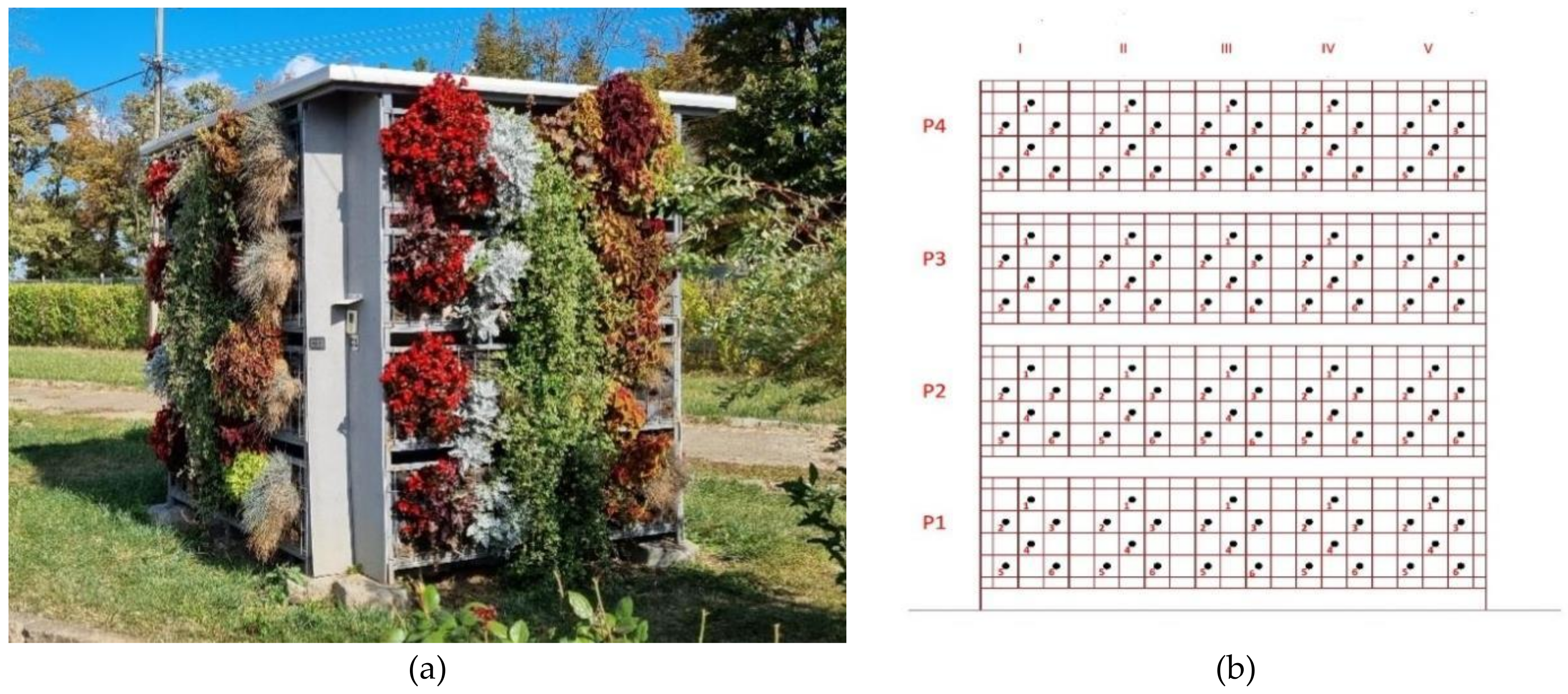
2.1. Experimental Site and Plant Materials

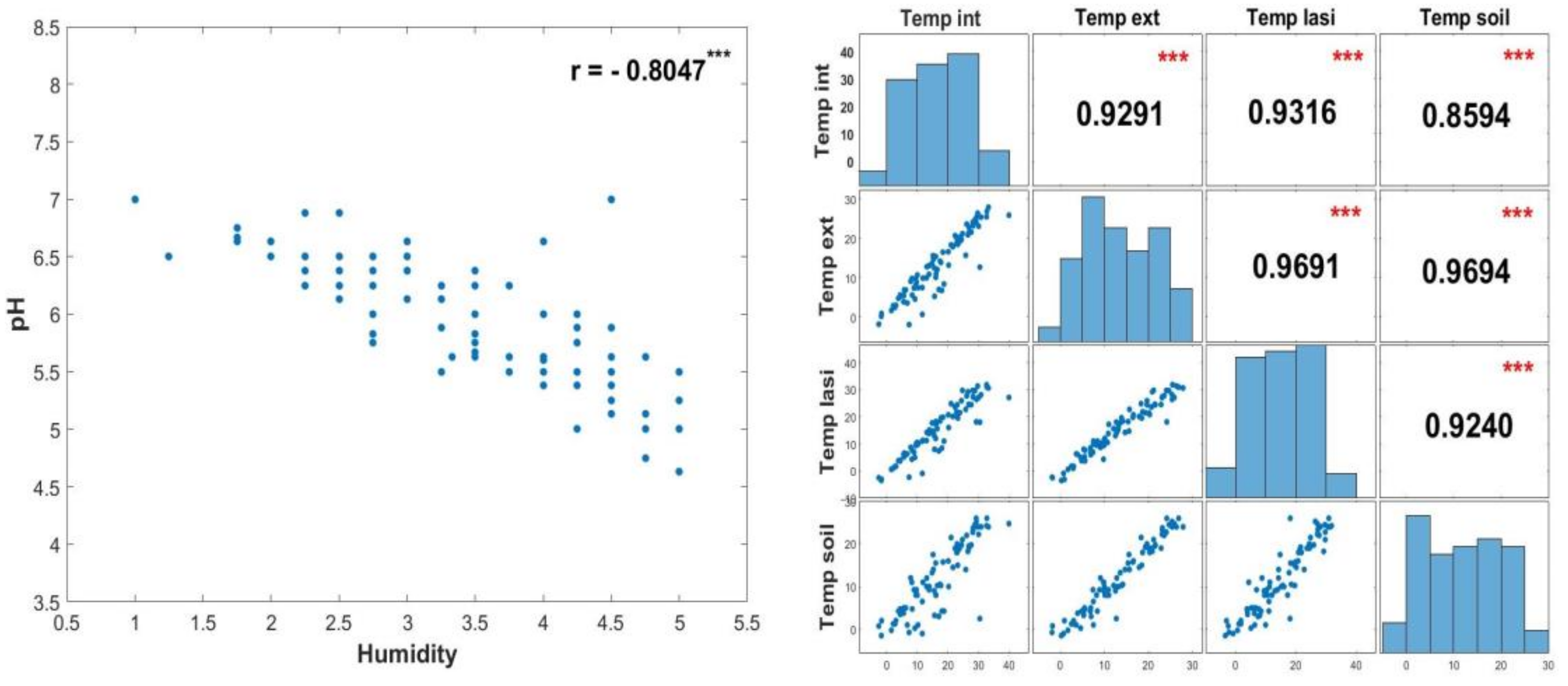
This study was initiated in northeastern Romania, which is part of the Eastern European climate. The experiment was conducted in the teaching field of the Floriculture Discipline, Faculty of Horticulture, Iasi University of Life Sciences (GPS decimal lat. N 47.1941, long. E 27.5555). The purpose of this experiment was to monitor the behavior of ornamental species that could be used successfully in various building roofing systems in Europe.

The green wall was made on independent levels, identical in shape and size, and arranged in layers on the experimental module. It was insulated on the inside and covered at the top with thermal insulation panels to suggest covering an insulated and unheated building. The size of a face (facade) is 2.00 m (length) × 2.40 m (height), each of which is oriented toward a cardinal point. The layers were filled with horticultural substrate, and planting was performed by drilling a slit in the geotextile foil (Geotex 50–Nortene) located on their outer face [42]. The flower species were planted on columns, and each facade was treated identically (see Figure 1). The vegetal material that we used was uniform, and its arrangement on the structure was uniform.

During the two-year period 2020–2021, we collected data from various measured features related to the green wall system, such as the plant coverage percentage of the system, inner and outer temperature of the system, temperature, humidity, and the pH of the soil. Starting from the available data, our target was to predict the plant coverage percentage of the system by considering different combinations of factors that might influence plant coverage. In our trial models, we have also taken into account various types of interactions between these factors. We will seek out to determine the importance of the interaction between the parameters that can influence the plant coverage percentage. It is possible that the soil registers the same temperature in different seasons, but the effect produced on the degree of plant coverage of the wall is totally different.

2.2. Measurements

During the study of the species planted vertically, we followed the percentage of attachment, degree of coverage, and behavior (biometric aspects and visual quality), depending on the cardinal orientation.

In addition, to determine the influence of environmental factors and the substrate used on the behavior of plants, the temperatures recorded in the area of the city of Iasi (Temp Iasi)—data received from the National Meteorology Center Iasi, the outdoor (Temp Ext) and indoor temperatures (Temp Int), the temperature (Temp soil), humidity (Hum), and pH of the substrate in which ornamental species were planted were monitored (

Table 1. Characteristics measured in 2020.

	Temp Int 2020 (°C)	Temp Ext 2020 (°C)	Temp Iasi 2020 (°C)	Humidity Soil 2020	Temp Soil 2020 (°C)	Plant Cover Green Wall (%) 2020
Mean	17.37	14.38	16.33	3.42	14.35	36.63
Minimum	−1.70	0.90	−3.10	1.00	−0.25	21.71
Maximum	39.90	26.90	31.80	5.00	28.25	71.05
CI mean	17.37 ± 1.59	14.38 ± 1.22	16.33 ± 1.53	3.42 ± 0.18	14.35 ± 1.29	36.63 ± 1.76

and

Table 2. Characteristics measured in 2021.

	Temp Int 2021 (°C)	Temp Ext 2021 (°C)	Temp Iasi 2021 (°C)	Humidity Soil 2021	Temp Soil 2021 (°C)	Plant Cover Green Wall (%) 2021
Mean	16.35	12.38	14.18	4.21	10.93	45.61
Minimum	−2.60	−1.90	−3.50	1.25	−2.00	13.82
Maximum	33.20	27.90	31.30	5.00	25.50	91.45
CI mean	16.35 ± 1.44	12.38 ± 1.25	14.18 ± 1.51	4.21 ± 0.14	10.93 ± 1.25	45.61 ± 3.57

).

Soil parameters were monitored using an RZ89 4 in 1 3.5∼9 pH Meter Digital Magnetic Soil Health Analyzer Machine Soil Moisture—Ammonitor Hygrometer Gardening Plant Tester. Data were collected during two calendar years (2020–2021), every three days, at the same time interval (11.30 AM to 01.30 PM).

The coverage was measured after three consecutive measurements. To measure soil moisture, the device used had the following scale: DRY+, DRY, NORMAL, WET, WET+. The transformation into numerical values was performed from 1 to 5, where 1 represents DRY+, and 5 represents WET+.

Over the two year period, the behavior of several perennial and annual flowering species was studied using one experimental module [42].

Given the favorable evolution of the plants used (Figure 1) on all façades of an experimental module, an attempt was made to find the best model that would predict the degree of coverage with plants. In 2020, the following flower species were found on the experimental scheme presented: Heuchera x hybrida ‘Fire Alarm’, Festuca glauca, Sedum spurium ‘Tricolor’, Carex testacea, and Polystichum aculeatum. Due to the low survival rate, in June-November 2020, Carex testacea was replaced by Begonia semperflorens (‘Big’). In 2021, on the façades of the experimental module, there were the following species: Begonia semperflorens, Heuchera x hybrida (‘Fire Alarm’), Cineraria maritima, Plectranthus fosteri, Coleus blumei, and Festuca glauca.

2.3. Model Development

In this section, we firstly describe how the data were preprocessed and the model variables were chosen, then we introduce the statistical methods employed in this paper: the multiple linear regression (MLR), the artificial neural networks (ANN), and the bootstrap method.

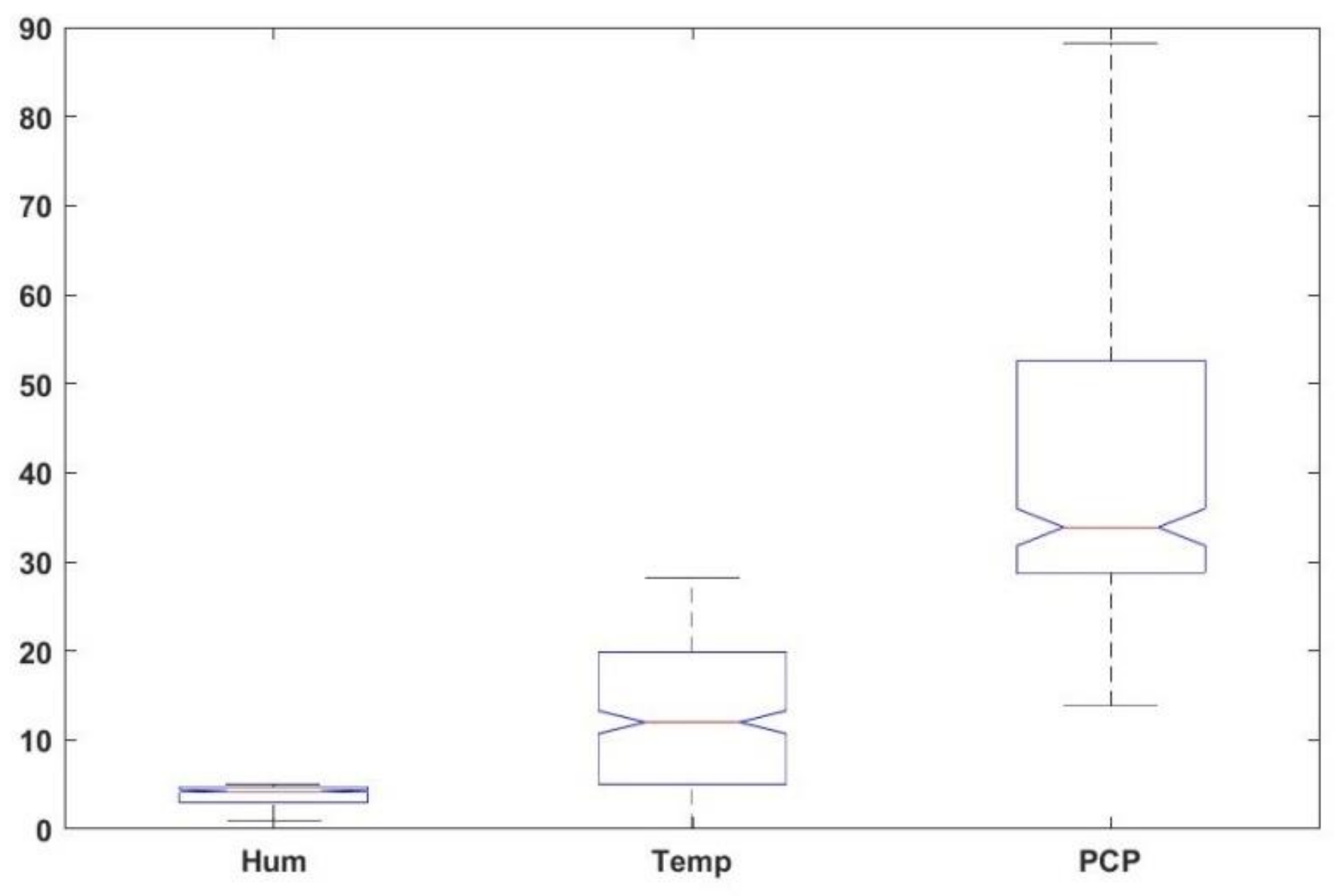
2.3.1. Data Preprocessing

The variable that we would prefer to explain in terms of the other measured features is the plant coverage percentage (PCP) of the façade of the experimental module. In order to extract the key predictors for PCP, and avoid multicolliniarity in the model, we have drawn scatter plots and calculated the linear correlation coefficients between the potential predictor variables. We have observed that some of the measured variables were highly correlated, and thus not all of them were considered in our models. For example, we have observed a significant negative linear correlation (see Figure 2) between the variables pH and humidity with the Pearson correlation coefficient $r=-0.8047\hspace{1em}(p=3.58\times {10}^{-21}).$ We have also observed that the recorded temperatures, Temp Int, Temp Ext, Temp Iasi and Temp soil, were highly linear correlated, as one can see from the scatter plots displayed Figure 2.

As a consequence, we have decided to keep only one of the temperature variables in the modelling, namely, the soil temperature. For the ease of notation, we shall simply call it Temp.

In the early stages, we thought that the height at which the plants are located on the vertical structure influences the degree of plant coverage (PCP), but only a negligible linear correlation was found. For this reason, the height of the plants on the wall system was not considered in any of the models.

In conclusion, out of all measured features, we decided to keep only humidity and temperature as possible predictors for the plant coverage percentage of the system, as each of them showed a significant linear correlation with the PCP. The other measured features were not considered in the modeling.

In the modeling stages, we also noticed that the plant coverage of the system was also dependent on other variables, which were not system-related, such as the time of the year when each observation was made, as well as the cardinal direction of each face of the system (the façade). Therefore, in order to obtain better predictions of plant coverage, we also included these variables in our models.

We finally arrived at the following shortlist of the independent (explanatory) variables, which were used in the regression model:

• The variable Hum, representing the soil humidity on a façade of the experimental module;
• The variable Temp, representing the soil temperature on a façade of the experimental module;
• The variable WkNo (week number), which keeps track of the time of the year when the data were recorded. It was coded to take values from 1 (the first week of January) to 52 (the last week of December).
• The variable Side represents the façade of the experimental module where the plants are grown. It could be N, E, S, or W, which are codified here as 1, 2, 3, and 4, respectively.

For the chosen variables, there were 324 observations available, 81 for each of the four façades of the experimental module. The data contain no missing values and no outliers, as one can also observe from Figure 3.

2.3.2. Multiple Linear Regression (MLR)

The general objective of regression analysis is to determine the relationship between two (or more) variables of interest so that we can gain information about one of them from the values of the other(s). In other words, regression analysis is a reliable method of identifying which variables (called stimuli, predictors, or explanatory variables) have an impact on a given feature (or variable) of interest, which is called the response or predicted/explained variable. When the response depends on a single stimulus, the regression is called simple regression. If the response depends on at least two stimuli, the regression is called multiple regression. The regression is called linear when the response depends linearly on the stimuli. The general equation for a multiple linear regression model with response $Y$ and $m$ stimuli, denoted by $X_k$, $k=1,\dots ,m$, is

$$Y=b_0+b_1{X}_1+b_2{X}_2+\dots +b_k{X}_k+b_m{X}_m,$$

(1)

where $b_k,k=1,\dots ,m,$ are called regression parameters. Each parameter $b_k$ represents the expected change in the response $Y$ associated with a 1-unit increase in $X_k$, while the other stimuli are held fixed. For a given model, the difference between the observed value for $Y$ and the value predicted by the model, $\widehat{Y},$ at the same given point, is called residual.

A useful model of multiple linear regression must satisfy the following assumptions: linear dependence of the response on the predictors, the homoscedasticity and the normality of the residuals, the independence of predictors, and no outliers in the data. The linear relationships between the response and any predictor can be spotted by plotting scatter diagrams, while residual plots are useful for checking the homoscedasticity and the normality of the residuals.

In a good MLR model, each predictor explains a part of the variation in the response variable. If predictor variables are not independent, but highly correlated, they will be “fighting” to explain the same part of the variation in the response variable, a phenomenon known as multicollinearity. Therefore, by employing highly correlated stimuli in the same model, this will not lead to a useful model. Usually, multicollinearity can be checked by calculating the correlation matrix of all the independent variables.

If the change in the mean value of $Y$ associated with a 1-unit increase in one independent variable (say, $X_1$) depends on the value of a second independent variable (say, $X_2$), then there is interaction between these two variables. One can incorporate this interaction into the MLR model by including the product of the two independent variables, $X_1{·X}_2$. As shall we see in the Section 3, our MLR model will contain such an interaction term between the variables Temp and WkNo.

In order to quantify how well a multiple linear regression model fits a dataset, we calculate the root-mean-square error (RMSE), the determination coefficient (R²), the adjusted R², and test the utility of the model (testing the significance of the model, as a whole). For a good model, one wishes RMSE to be small, R² to be close to 1, and the adjusted R² to be fairly close (but less) to R², and the F-statistic for the utility test should be large enough.

For a specific set of predictor values within the data range, say $x_1^{*},x_2^{*},\dots ,x_m^{*}$, the expected value of $Y$ in (1) is

$${\widehat{Y}}_{*}={{\widehat{b}}_0+\widehat{b}}_1{x}_1^{*}+{\widehat{b}}_2{x}_2^{*}\dots \dots +{\widehat{b}}_m{x}_m^{*}.$$

(2)

Then, a –00(1 − α)% confidence interval for $Y_{*}$ (the mean response in Y) is

$${\widehat{Y}}_{*}\pm t_{1-\mathsf{\alpha }/2;n-m-1}\times \mathit{SE}\left({\widehat{Y}}_{*}\right),$$

(3)

where $t_{1-\mathsf{\alpha }/2;n-m-1}$ is the $1-\frac{\mathsf{\alpha }}{2}$ quantile for the Student distribution $t(n-m-1)$, and $\mathit{SE}\left({\widehat{Y}}_{*}\right)$ is the standard error of the estimator ${\widehat{Y}}_{*}$. For more details on the multiple linear regression models, see [43]. The MLR model was processed with the Statistical Toolbox in MATLAB.

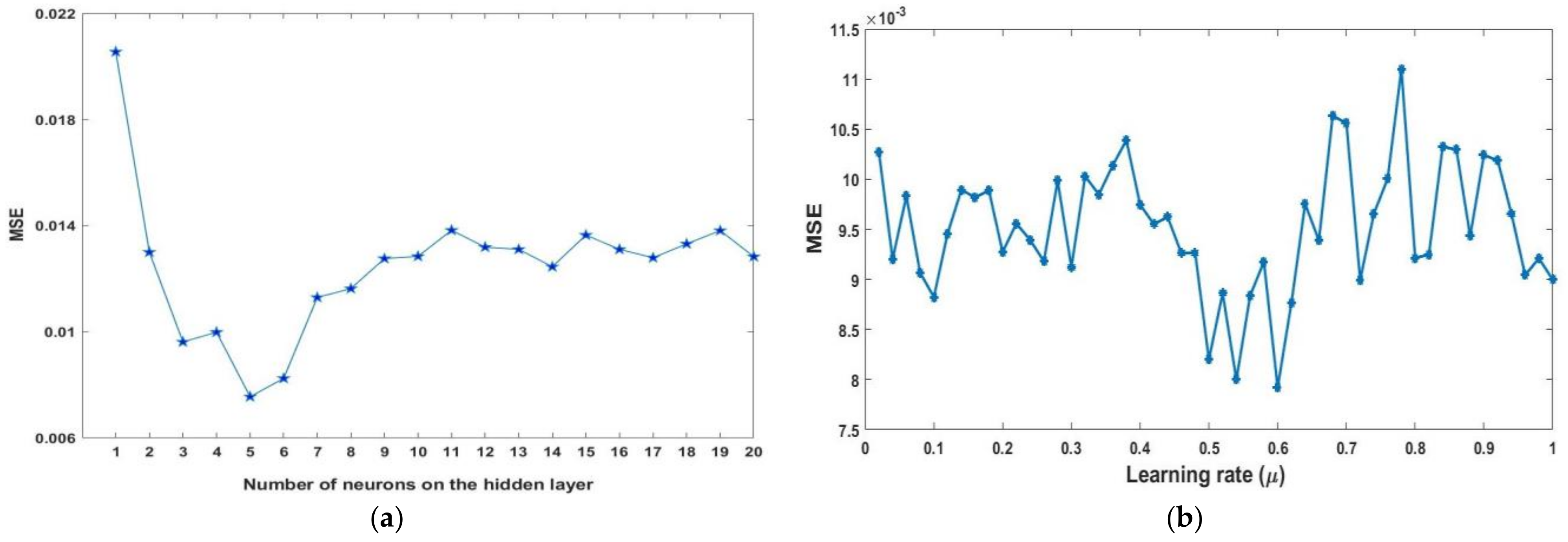
2.3.3. Artificial Neural Networks (ANNs)

A neural network is a machine learning technique that teaches computers to process data in a way that is inspired by the human brain. It uses interconnected nodes (called neurons) in a layered structure, aiming to resemble the human brain. ANNs are designed in such a way that computers can learn from their mistakes and improve continuously. They are powerful and versatile tools that can be used in various situations, such as: function approximation, classification, speech recognition, pattern recognition, finding clusters or regularities in the data, etc.

Similar to MLR methods, ANNs are able to learn and to generalize relations between input and output data from examples presented to the network. The main advantage of using ANNs for predictions is that the a priori assumptions related to the predictors and responses are not necessary, as is the case for MLR. However, while the relations between input and output data that are modeled by multi-linear regression models that can be expressed by some equation (as the one shown above, whose parameters can be easily interpreted), the relations learned by an ANN are hidden in its neural architecture and cannot be easily expressed in traditional mathematical terms.

An artificial neural network consists of a number of highly interconnected nodes (or neurons), organized in layers. The minimum number of layers of an ANN is two (an input layer and an output layer), but a multi-layered ANN can also have one or more hidden layers. Figure 4 displays an example of a neural network having: an input layer with four neurons, one hidden layer with five neurons, and an output layer with one neuron. The neurons in the input layer receive data from the outside world, and then they transmit it forward via the weighted connections to the neurons in the next layer (which, in the above example, is the hidden layer). This information is aggregated and modulated by an activation function, which can be set for each node in part. If the information that arrives at each node in the hidden layer exceeds some given threshold, the neuron becomes activated and can transmit the acquired information forward to the neurons in the next layer. The process of transmitting continues forward to the next layer, and so on until the last layer is reached.

A neural network in which the data is transmitted only forward through all the layers and has no feed-back loops is called a feed-forward multi-layer ANN (shortly, FFNN). For other types of ANNs, one can see [44]. Once the output layer is reached, the neurons in the output layer will give the results. The discrepancy between the outputs of the network and the desired targets is measured by an appropriate cost function. Using a specific back-propagation algorithm, the weights of the network are adjusted (process that is called learning) at each iterative step in order to minimize this cost function. In this paper, the cost function (or performance) is the mean squared error (MSE) between the outputs of the network and desired (observed) values.

Motivated by the known fact that a feed-forward neural network with only one hidden layer can approximate any function to arbitrary accuracy (the universal approximation theorem, see [45]), it is reasonable to consider this type of network architecture as a candidate model to determine the best nonlinear dependence of a response variable $Y$ on a set of stimuli $X_k$, $k=1,\dots ,m$. For this reason, we shall use, in this paper, only feed-forward ANNs with one hidden layer as the basic approximation elements in finding the best nonlinear dependence in the data.

We have considered here a FFNN with three layers, having four nodes on the input layer (which represent our model predictors), only one hidden layer, and an output layer with only one neuron, representing the model response variable. The number of nodes in the hidden layer was varied between 1 and 20, and the learning rate was varied from 0.02 to 1.0 in increments of 0.02 (see Figure 5). Finally, the optimal number of neurons on the hidden layer and the optimal learning rate were selected using a trial-and-error method, as this relates to the values that will give the best ANN performance. The mean squared error (MSE),

$$\mathrm{MSE}=\frac{1}{n}\sum _{k=1}^n{\left({\mathit{out}}_k-{\mathit{target}}_k\right)}^2$$

was selected as the performance function of the ANN. The smaller the MSE value, the better the performance of the ANN. As displayed in Figure 4, we have found that the optimal number of neurons on the hidden layer is 5, and the optimal learning rate is $\mu =0.6$.

For the computer implementation of the ANN, we have employed the neural network toolbox in MATLAB. We have taken the tansig activation function for the neurons in the hidden layers and a linear activation function in the output node. The ANN is trained using a Bayesian regularization back-propagation algorithm. We chose Bayesian regularization because it has a better performance than Levenberg-Marquardt back-propagation for small datasets. Moreover, the Bayesian regularization does not require a validation dataset, leaving more data available for training. The function trainbr that performs Bayesian regularization in Matlab disables validation stops by default. This is due to the fact that validation is usually used as a form of regularization, but trainbr has its own form of validation built into the algorithm (for more details, see [46]).

Once the data are presented to the network, they are split into two parts, one for training and one for testing. The input nodes are fed with the values of the predictors. Every newly created ANN starts with different initial conditions, such as initial weights and biases, as well as different division of the training and test datasets. As a consequence, the different initial conditions can lead to very different solutions for the same problem. Moreover, for certain initial conditions for ANN, it is possible to fail in obtaining realistic solutions for a given problem. As argued in [47], a good idea to avoid this inconvenience is to train several neural networks to ensure that a network with good generalization is found. Furthermore, by retraining each network, one can verify a robust network performance. As detailed in the Section 3, we shall train 50 ANNs on the given data, starting from different initial weights and biases, and with different divisions for the training and test data sets. Each of these ANNs is then retrained five times to ensure a good generalization. The ANN with the best performance (the lowest MSE) overall is then traced, and its weights are used in making predictions for unseen data.

When doing predictions with ANNs, there is no indication of uncertainty about these predictions. Therefore, we have used the bootstrap method (presented below) to construct confidence intervals for predictions.

2.3.4. The Bootstrap Method for Confidence Intervals

Bootstrapping is a resampling with replacement technique used in estimating standard errors for the statistics of interest, based on which one can build confidence intervals. The method is especially useful when classical confidence is not applicable (e.g., the volume of the sample data is small, assumptions for data distribution are not met), and it can give very good results in the case of complicated nonlinear statistics. In the bootstrap method, the sample data are regarded as a statistical population, from which we can extract various samples, in order to gather more information about the sample.

Let us say that θ is the parameter of interest, for which we seek a confidence interval. Based on a sample of volume n, the steps in a bootstrap method for building a confidence interval for θ are:

• choose the number $B\le n^n$ of Bootstrap samples of size $n$ to perform;
• resample with replacement of the given dataset, obtaining B Bootstrap samples of volume $n$
• for each bootstrap sample, calculate the statistic of interest, say ${\widehat{\theta }}_b^{\mathrm{*}}$, $b\mathrm{}=1,2,\dots ,B$.
• calculate the mean $\overline{{\widehat{\theta }}^{\mathrm{*}}}$ and the standard deviation $s_{{\widehat{\theta }}^{\mathrm{*}}}$ of the calculated sample statistic;
• write a 100(1 − α)% confidence interval for θ as follows:

$$\overline{{\widehat{\theta }}^{*}}\pm z_{1-\mathsf{\alpha }/2}\times s_{{\widehat{\theta }}^{*}},$$

(4)

where $z_{1-\mathsf{\alpha }/2}$ is the $(1-\mathsf{\alpha }/2)$ quantile for the standard normal distribution.

This method has some advantages: simplicity, easiness to derive estimates of standard errors and confidence intervals for complex estimators, and avoiding the cost of repeating experiments to obtain sample data. However, this method also has some disadvantages: final results may depend on the original sample, and it is time-consuming and difficult to automate using traditional statistical computer packages. For more details on the bootstrap method, see [41].

In the Section 3, we have constructed a confidence interval for the predictions given by the constructed ANN, by resampling $B=100$ times the given dataset and then passing the samples through the ANN, to obtain a set of predictions. For these predictions, we have calculated the mean and the standard deviation, based on which the confidence interval was built.

3. Results

3.1. A Multiple Linear Regression Model (MLR)

In this section, our aim is to obtain a multiple linear regression model that fits well with the available, such that all the model parameters are significant at level 0.05, and the model can be useful in doing predictions.

By trial and error, we have built quite a few multiple linear regression models that involve the four above mentioned predictors, Hum, Temp, WkNo, and Side, by looking at the model performances, such as the significance of the model parameters, MSE, R², adjusted R², and the utility of the model. We have also observed that the influence of Temp on the mean value of the PCP depends upon the values WkNo. In other words, the mean plant coverage percentage at a given temperature (say, 18 °C) depends on whether that temperature is observed in March or in July. Therefore, we have also taken into account an interaction term between the variables Temp and WkNo in our modelling, as it fits better the available data.

We can symbolically write this model as:

$$\mathrm{PCP}~\mathit{Hum}+\mathit{Temp}+\mathit{WkNo}+\mathit{Side}+\mathit{Temp}·\mathit{WkNo},$$

(5)

The coefficients and other statistical characteristics of this model are presented in

Table 3. Statistics for the multiple linear regression model.

	Estimated Parameter	Standard Error	Test Statistic	p-Value
Hum	5.0908	0.63696	7.9942	2.4462 × 10−14
Temp	−1.2014	0.25157	−4.7755	2.7369 × 10−6
WkNo	0.62273	0.06814	9.1319	7.5291 × 10−18
Side	1.90730	0.66521	2.8673	0.0044126
Temp·WkNo	0.03804	0.00813	4.6797	4.2531 × 10−6

.

The model was constructed using 324 observations. Other relevant statistics for this model are as follows: the error degree of freedom is 319, $\mathrm{RMSE}=14.6$ (which is relatively small), $R^2$= 0.5549 (meaning that 55.49% of the variation in PCP can be explained by the MLR model), and $\mathit{adjusted}$= 0.5493 (which is close to $R^2$, meaning that the number of variables in the model is not too high). The F-statistic value for testing the utility of the model is $F=79.238$, and the corresponding p-value is $p=7.5551{\times 10}^{-54}$, proving the model to be useful.

Based on the fitted parameters, the model is expressed as follows:

$$\mathrm{PCP}=5.0908·\mathit{Hum}-1.2014·\mathit{Temp}+0.62273·\mathit{WkNo}+1.9073·\mathit{Side}+0.03804·\mathit{Temp}·\mathit{WkNo}$$

(6)

We shall make here some additional comments on the model:

• From the displayed p-values, we see that all the model coefficients are significant at any significance level less than 0.005.
• An increase of one unit in humidity will determine an increase of almost 5.1% in plant coverage percentage;
• An increase of 1 °C in temperature will determine a decrease of almost 1.21% in plant coverage percentage;
• The variable represented by the week of the year when the data were collected had a significant influence on the plant coverage percentage.
• The choice of the experimental module façade had a significant influence (of magnitude 1.9073) on the plant coverage percentage.
• The coefficient 0.03804 suggests that, for each fixed week number, an increase of 1 °C in soil temperature will determine an increase of almost 4% in plant coverage percentage. The interaction between these two parameters, the soil temperature and the week of the year, is important for the model. It is possible that the soil registers the same temperature in different seasons, but the effect produced on the degree of plant coverage of the wall is totally different (for example, the soil can have temperatures of 10 °C both on a summer week and a winter week, and the influence on the PCP can be totally different).

3.2. Confidence Interval for the PCP Based on the Multiple Linear Regression

The multiple linear regression model (6) for plant development on the green wall can be employed to predict how the independent variables (humidity, soil temperature, cardinal orientation, and the week of the year) influence the percentage of plant coverage. Let us consider the following set of values for the predictors, which are in the data range: for example, Hum = 4, Temp = 23, WkNo = 25, and Side = 1 (i.e., the north-facing facade). Then, by using Formula (6), the predicted value of PCP was 32.07%. The t-quantile corresponding to the model is $t_{0.975,318}=1.9675,$ and the standard deviation of the estimate is $\mathit{SE}\left({\widehat{Y}}_{*}\right)=1.8813$. Using the Formula (3), the 95% confidence interval for the mean PCP is:

$$[28.37\mathrm{\%},\hspace{1em}35.77\mathrm{\%}].$$

(7)

Later, we shall compare this confidence interval with the one obtained via the artificial neural network approach. Figure 6 displays the values predicted by the model and the actual observed values for a fixed week number (25) and fixed side (1) of the experimental structure.

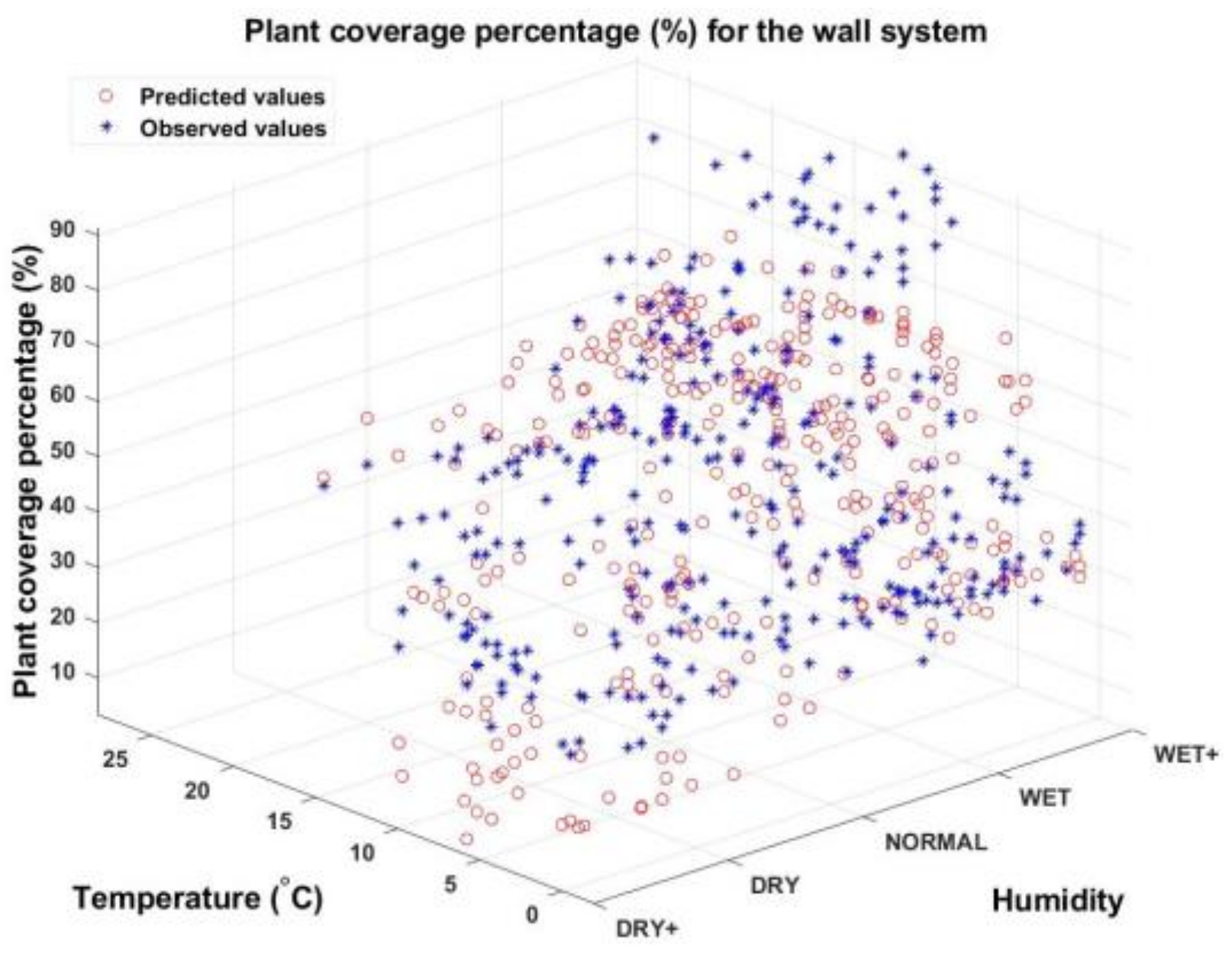
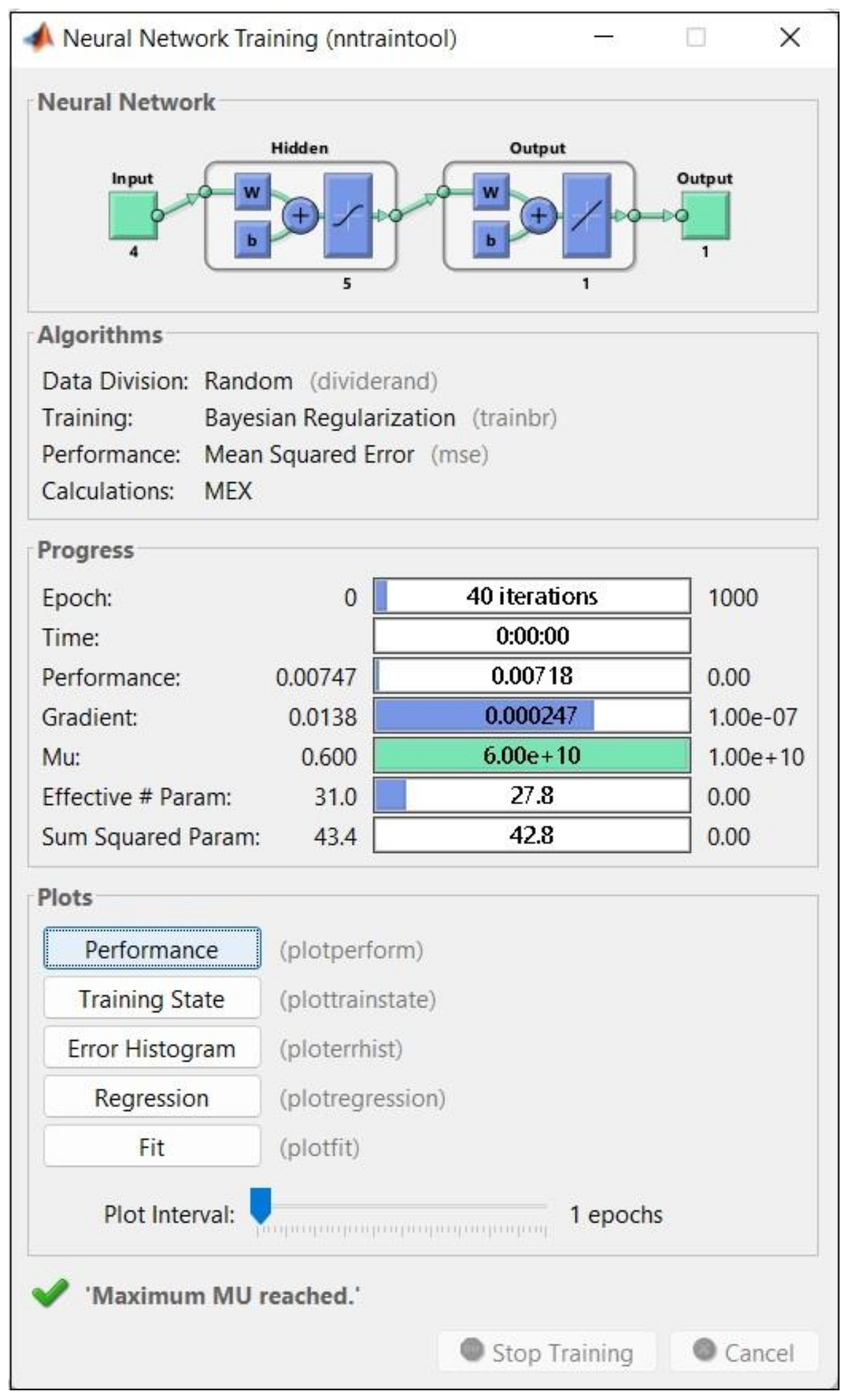
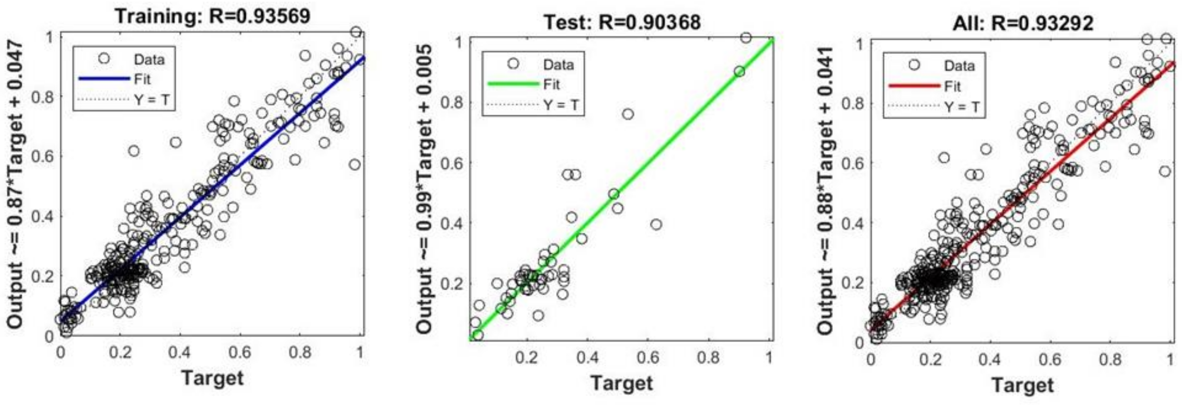
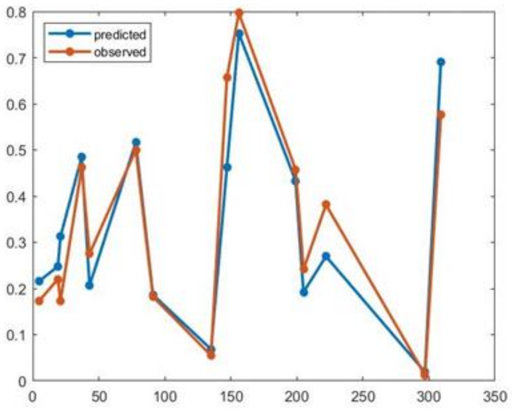
3.3. An Artificial Neural Network Model (ANN)

The designed ANN, which is illustrated in Figure 4, is made of: one input layer with four neurons, one hidden layer with five neurons, and one output layer with one neuron. The motivation for this specific architecture was presented in Section 2.3.3. The neural network was fed with the available data for four predictors: soil humidity (Hum), soil temperature (Temp), week of the year (WkNo), and the cardinal orientation of the structure face (Side). Based on these four predictors, our aim is to estimate (both punctually and by a confidence interval) the plant coverage percentage (PCP). The confidence interval was constructed using the bootstrap method.

The activation function employed for the hidden layer was the tansig function,

$$f(x)=\mathit{tansig}(x)=\frac{2}{1+e^{-2x}}-1.$$

(8)

For the output layer, we have considered the purelin transfer function,

$$g\left(x\right)=\mathit{purelin}\left(x\right)=x.$$

(9)

Denote by $v_{ij}$, $b_j$ ($i=1,\dots ,4,j=1,\dots ,5$) the weights and the biases (respectively), from the input layer to the hidden layer, and by $w_j(j=1,\dots ,5$), $b_0$ the weights and the bias (respectively) from the hidden layer to the output layer. Then, with the notations for the activation functions that were mentioned above, the external signal out that is produced by the neural network through its layers is

$$\mathit{out}=g\left(b_0+\sum _{j=1}^5{w}_{j}f\left(b_j+\sum _{i=1}^4{v}_{ij}{x}_i\right)\right)$$

(10)

Note that the ANN model Formula (10) for (PCP) is much more complex than the corresponding Formula (6) for the MLR model.

The dataset was randomly divided into two separate sets using the dividerand function in MATLAB, such that 85% of the data values were used for the training set, and 15% were used for the testing set. As also mentioned in Section 2.3.3, the backpropagation algorithm with Bayesian backpropagation was used for ANN training.

The nntraintool in MATLAB was used to monitor the training progress (Figure 7).

For faster training, the inputs (Hum, Temp, WkNo, Side) and the output PCP were normalized using the min-max normalization. The normalization of a generic data value $x_i$ from dataset $x$ is

$$z_i=\frac{x_i-\min \left(x\right)}{\max \left(x\right)-\min \left(x\right)}\in [0,1].$$

(11)

As explained in Section 2.3.3, we have trained 50 ANNs, each neural network having the same particular architecture that we have mentioned above, and then we traced down the neural network with the best performance. This optimal neural network was used in making predictions for the response variable.

Figure 8 displays the linear regressions of the optimal network output values (predictions) versus the observed values (target) obtained in training, testing, and overall.

As shown in Figure 8, the linear correlation between the output values (given by the model) and the observed values in the database is larger than 0.9, indicating a good fit of the data. Figure 9 shows the distribution of the errors, which is fairly normal. A set of 15 data values was intentionally excluded from the training set for testing purposes.

Figure 10 displays 15 values predicted by the ANN model (outputs) and the actual values that were observed (targets), showing a very good fit. The mean squared error (MSE) between the outputs and targets is $\mathrm{MSE}=0.0075493$.

3.4. Confidence Interval for the PCP Based on Artificial Neural Networks

The confidence interval that we build here is based on the bootstrap method [41], which is a statistical technique based on resampling a dataset with replacement.

This technique is based on training a number of ANNs, which can lead to lower estimation errors with regard to a single ANN. To train each of these networks, we employed randomly selected samples from the initial dataset.

We begin by considering our dataset as a sample obtained from an underlying distribution. We then resampled the dataset with replacement $B=100$ times and used each of these resamples as training data for an artificial neural network with the architecture presented in the previous section. For each of these 100 resamples, we trained 50 artificial neural networks and then chose the neural network that had the best performance (measured here as MSE) on that specific resampled dataset. This chosen neural network will give a prediction based on a specific set of values for the predictors. For comparison purposes, we use the same choice of input data as in Section 3.2, that is, Hum = 4, Temp = 23, WkNo = 25, and Side = 1.

Consequently, each resampled dataset $x$ produces an estimated value for the plant cover percentage, resulting in a total of 100 predictions.

If $y_1\left(x\right),y_2\left(x\right),\dots ,y_B\left(x\right)$ are these predictions, then:

-

the bootstrap mean is

$${\widehat{y}}_{\mathit{boot}}(x)=\frac{1}{B}\sum _{b=1}^B{y}_b\left(x\right)$$

(12)

-

the bootstrap standard deviation is

$${\widehat{\sigma }}_{\mathit{boot}}(x)=\sqrt{\frac{1}{B-1}\sum _{b=1}^B{\left({\widehat{y}}_{\mathit{boot}}\right(x)-y_b(x\left)\right)}^2}$$

(13)

By using the Formula (4), we write the $95\mathrm{\%}$ confidence interval as:

$$\left[{\widehat{y}}_{\mathit{boot}}\right(x)-1.96·{\widehat{\sigma }}_{\mathit{boot}}\left(x\right),{\widehat{y}}_{\mathit{boot}}\left(x\right)+1.96·{\widehat{\sigma }}_{\mathit{boot}}\left(x\right)$$

(14)

The numerical values that we obtained are: ${\widehat{y}}_{\mathit{boot}}\left(x\right)$ = 31.44 (the bootstrap mean), and ${\widehat{\sigma }}_{\mathit{boot}}\left(x\right)$ = 1.25 (the bootstrap standard deviation). Therefore, the bootstrap confidence interval for PCP is:

$$[28.99\mathrm{\%},\hspace{1em}33.89\mathrm{\%}].$$

(15)

We see that this confidence interval for PCP has a smaller length (and thus is more precise) than that the confidence interval (7) obtained via the multiple linear regression model.

In other words, for week 25, with soil humidity equal to 4, as well as soil temperature of 23 °C on the north-facing facade, the percentage of plant coverage will be determined more precisely using the ANN method when compared to the MLR.

From our perspective, it is clear that the model obtained by ANN is superior to the one obtained by MLR because, in reality, the dependence between the degree of coverage (PCP) and the rest of the analyzed variables is not entirely linear, and the ANN model has the ability capture these non-linearities.

4. Conclusions

In this study, we derived point estimations and confidence intervals for the percentage of plant coverage of a vertical green system using two models: a multiple linear regression model and an artificial neural network, with the aim of comparing them. This study proves that both approaches, the multiple linear regression and the artificial neural network, can be used in the landscape field, but for more accurate predictions, the use of artificial neural networks could provide even better results due to the capability of detecting unseen relationships between variables. The advantage of the MLR is the easiness to interpret the results and the interdependencies between variables. It also has an in-hand formula, based on which one can make predictions, and one can assess the uncertainty these predictions. The advantage of the neural network method is that it does not need any mathematical relationship between input and output data to depict even more features from the original data than the MLR. However, since the ANN is regarded as a black box model, we could not determine the precise relationships between the predictors and response, which is a rather complicated one. Another drawback of the ANN method is that we do not know which of the predictors we used had more (or less) influence on the predictions for PCP. Another inconvenient fact is that, when doing predictions via ANN, there is no indication of the degree of uncertainty associated with these predictions. However, in the approach we follow here, we obtain an estimate of this uncertainty via the bootstrap method.

In order to develop a robust ANN, we have carefully estimated the number of layers, the number of neurons on the hidden layer, and the learning rates for the ANN. It is a known fact that, if the number of neurons in the hidden layer is too low, then the ANN cannot reflect nonlinearity within the training data. On the other hand, if there are too many neurons on the hidden layer, then the ANN has an overfitting problem, leading to a lack of generalizability. Moreover, we have trained several ANNs, with different divisions of training and test datasets, to ensure that a network with good generalization is found.

The models that we presented here have their own limitations. Usually, in practice, the percentage of plant coverage is difficult to predict, as it depends on many other variables, which were not considered here, such as: the weather conditions, the size and the orientation of the wall structure, human intervention, light intensity, the characteristics of the floral species that were used, the type of green wall system, the climate, etc. The data we have obtained here were under fairly normal weather conditions, in the climate specific to the north-east of Romania, on a wall structure facing in all four cardinal directions, which was not shaded by other objects, such as trees or houses. The models might not be applicable if, for example, the structure was always facing north, or if it was under a different climate, or if there were extreme weather conditions, or if the structure was (at least) partially shaded by other objects, etc.

The usefulness of our analysis derives primarily from the fact that most beneficiaries want to know, right from the design phase, how long it will take for the chosen plants to reach significant decorative potential. They would also appreciate the usefulness of predicting the percentage of plant coverage of a green wall system with a high degree of accuracy in the case of organizing outdoor exhibitions or other similar projects.

The information collected from the analyzed models reveals to the specialists in the field which parameters or combinations of parameters must be followed in order to maintain the visual effects of the green wall for as long as possible. We believe that the results obtained in this study will lead to new research on green walls in the north-eastern climate zone of Europe.

References

1. Peschardt, K.K.; Schipperijn, J.; Stigsdotter, U.K. Use of Small Public Urban Green Spaces (SPUGS). Urban For. Urban Green. 2012, 11, 235–244. [Google Scholar] [CrossRef]
2. Akbari, H.; Pomerantz, M.; Taha, H. Cool Surfaces and Shade Trees to Reduce Energy Use and Improve Air Quality in Urban Areas. Sol. Energy 2001, 70, 295–310. [Google Scholar] [CrossRef]
3. Yang, J.; Yu, Q.; Gong, P. Quantifying Air Pollution Removal by Green Roofs in Chicago. Atmos. Environ. 2008, 42, 7266–7273. [Google Scholar] [CrossRef]
4. Strohbach, M.W.; Arnold, E.; Haase, D. The Carbon Footprint of Urban Green Space—A Life Cycle Approach. Landsc. Urban Plan. 2012, 104, 220–229. [Google Scholar] [CrossRef]
5. Peschardt, K.K.; Stigsdotter, U.K. Associations between Park Characteristics and Perceived Restorativeness of Small Public Urban Green Spaces. Landsc. Urban Plan. 2013, 112, 26–39. [Google Scholar] [CrossRef]
6. Price, A.; Jones, E.C.; Jefferson, F. Vertical Greenery Systems as a Strategy in Urban Heat Island Mitigation. Water Air Soil Pollut. 2015, 226, 247. [Google Scholar] [CrossRef]
7. Ghazalli, A.J.; Brack, C.; Bai, X.; Said, I. Physical and Non-Physical Benefits of Vertical Greenery Systems: A Review. J. Urban Technol. 2019, 26, 53–78. [Google Scholar] [CrossRef]
8. Chiesura, A. The Role of Urban Parks for the Sustainable City. Landsc. Urban Plan. 2004, 68, 129–138. [Google Scholar] [CrossRef]
9. Wolch, J.R.; Byrne, J.; Newell, J.P. Urban Green Space, Public Health, and Environmental Justice: The Challenge of Making Cities “Just Green Enough”. Landsc. Urban Plan. 2014, 125, 234–244. [Google Scholar] [CrossRef] [Green Version]
10. Currie, B.A.; Bass, B. Estimates of Air Pollution Mitigation with Green Plants and Green Roofs Using the UFORE Model. Urban Ecosyst. 2008, 11, 409–422. [Google Scholar] [CrossRef]
11. Perez-Urrestarazu, L.; Fernandez-Canero, R.; Franco-Salas, A.; Egea, G. Vertical Greening Systems and Sustainable Cities. J. Urban Technol. 2015, 22, 65–85. [Google Scholar] [CrossRef]
12. Frumkin, P. Beyond Toxicity—Human Health and the Natural Environment. Am. J. Prev. Med. 2001, 20, 234–240. [Google Scholar] [CrossRef] [PubMed]
13. Sheweka, S.M.; Mohamed, N.M. Green Facades as a New Sustainable Approach Towards Climate Change. In Proceedings of the Terragreen 2012: Clean Energy Solutions for Sustainable Environment (Cesse), Beirut, Lebanon, 16–18 February 2012; Salame, C., Aillerie, M., Khoury, G., Eds.; Elsevier Science Bv: Amsterdam, The Netherlands, 2012; Volume 18, pp. 507–520. [Google Scholar]
14. Eumorfopoulo, E.A.; Kontoleon, K.J. Experimental Approach to the Contribution of Plant-Covered Walls to the Thermal Behaviour of Building Envelopes. Build. Environ. 2009, 44, 1024–1038. [Google Scholar] [CrossRef]
15. Synnefa, A.; Dandou, A.; Santamouris, M.; Tombrou, M.; Soulakellis, N. On the Use of Cool Materials as a Heat Island Mitigation Strategy. J. Appl. Meteorol. Climatol. 2008, 47, 2846–2856. [Google Scholar] [CrossRef]
16. Zinzi, M.; Agnoli, S. Cool and Green Roofs. An Energy and Comfort Comparison between Passive Cooling and Mitigation Urban Heat Island Techniques for Residential Buildings in the Mediterranean Region. Energy Build. 2012, 55, 66–76. [Google Scholar] [CrossRef]
17. Djedjig, R.; Bozonnet, E.; Belarbi, R. Experimental Study of the Urban Microclimate Mitigation Potential of Green Roofs and Green Walls in Street Canyons. Int. J. Low-Carbon Technol. 2015, 10, 34–44. [Google Scholar] [CrossRef] [Green Version]
18. Wong, N.H.; Chen, Y.; Ong, C.L.; Sia, A. Investigation of Thermal Benefits of Rooftop Garden in the Tropical Environment. Build. Environ. 2003, 38, 261–270. [Google Scholar] [CrossRef]
19. Takebayashi, H.; Moriyama, M. Surface Heat Budget on Green Roof and High Reflection Roof for Mitigation of Urban Heat Island. Build. Environ. 2007, 42, 2971–2979. [Google Scholar] [CrossRef] [Green Version]
20. Teemusk, A.; Mander, U. Greenroof Potential to Reduce Temperature Fluctuations of a Roof Membrane: A Case Study from Estonia. Build. Environ. 2009, 44, 643–650. [Google Scholar] [CrossRef]
21. Cheng, C.Y.; Cheung, K.K.S.; Chu, L.M. Thermal Performance of a Vegetated Cladding System on Facade Walls. Build. Environ. 2010, 45, 1779–1787. [Google Scholar] [CrossRef]
22. Kozamernik, J.; Rakuša, M.; Nikšič, M. How Green Facades Affect the Perception of Urban Ambiences: Comparing Slovenia and the Netherlands. Urbani Izziv 2020, 31, 88–100. [Google Scholar] [CrossRef]
23. Tsantopoulos, G.; Varras, G.; Chiotelli, E.; Fotia, K.; Batou, M. Public Perceptions and Attitudes toward Green Infrastructure on Buildings: The Case of the Metropolitan Area of Athens, Greece. Urban For. Urban Green. 2018, 34, 181–195. [Google Scholar] [CrossRef]
24. Gantar, D.; Kozamernik, J.; Erjavec, I.S.; Koblar, S. From Intention to Implementation of Vertical Green: The Case of Ljubljana. Sustainability 2022, 14, 3198. [Google Scholar] [CrossRef]
25. Sari, A.A. Thermal Performance of Vertical Greening System on the Building Facade: A Review. AIP Conf. Proc. 2017, 1887, 020054. [Google Scholar] [CrossRef] [Green Version]
26. Feng, L.-H.; Lu, J. The Practical Research on Flood Forecasting Based on Artificial Neural Networks. Expert Syst. Appl. 2010, 37, 2974–2977. [Google Scholar] [CrossRef]
27. Wu, X.D.; Cao, H.X.; Flitman, A.; Wei, F.Y.; Feng, G.L. Forecasting Monsoon Precipitation Using Artificial Neural Networks. Adv. Atmos. Sci. 2001, 18, 950–958. [Google Scholar] [CrossRef]
28. Sohn, S.H.; Oh, S.C.; Yeo, Y.K. Prediction of Air Pollutants by Using an Artificial Neural Network. Korean J. Chem. Eng. 1999, 16, 382–387. [Google Scholar] [CrossRef]
29. Erdil, A.; Arcaklioglu, E. The Prediction of Meteorological Variables Using Artificial Neural Network. Neural Comput. Appl. 2013, 22, 1677–1683. [Google Scholar] [CrossRef]
30. Runge, J.; Zmeureanu, R. Forecasting Energy Use in Buildings Using Artificial Neural Networks: A Review. Energies 2019, 12, 3254. [Google Scholar] [CrossRef] [Green Version]
31. Lehnert, L.W.; Meyer, H.; Wang, Y.; Miehe, G.; Thies, B.; Reudenbach, C.; Bendix, J. Retrieval of Grassland Plant Coverage on the Tibetan Plateau Based on a Multi-Scale, Multi-Sensor and Multi-Method Approach. Remote Sens. Environ. 2015, 164, 197–207. [Google Scholar] [CrossRef]
32. Al-Saif, A.M.; Abdel-Sattar, M.; Eshra, D.H.; Sas-Paszt, L.; Mattar, M.A. Predicting the Chemical Attributes of Fresh Citrus Fruits Using Artificial Neural Network and Linear Regression Models. Horticulturae 2022, 8, 1016. [Google Scholar] [CrossRef]
33. Abdipour, M.; Younessi-Hmazekhanlu, M.; Ramazani, S.H.R.; Omidi, A.H. Artificial Neural Networks and Multiple Linear Regression as Potential Methods for Modeling Seed Yield of Safflower (Carthamus Tinctorius L.). Ind. Crops Prod. 2019, 127, 185–194. [Google Scholar] [CrossRef]
34. Abdel-Sattar, M.; Al-Obeed, R.S.; Aboukarima, A.M.; Eshra, D.H. Development of an Artificial Neural Network as a Tool for Predicting the Chemical Attributes of Fresh Peach Fruits. PLoS ONE 2021, 16, e0251185. [Google Scholar] [CrossRef] [PubMed]
35. Huang, X.; Chen, T.; Zhou, P.; Huang, X.; Liu, D.; Jin, W.; Zhang, H.; Zhou, J.; Wang, Z.; Gao, Z. Prediction and Optimization of Fruit Quality of Peach Based on Artificial Neural Network. J. Food Compos. Anal. 2022, 111, 104604. [Google Scholar] [CrossRef]
36. Abdel-Sattar, M.; Al-Saif, A.M.; Aboukarima, A.M.; Eshra, D.H.; Sas-Paszt, L. Quality Attributes Prediction of Flame Seedless Grape Clusters Based on Nutritional Status Employing Multiple Linear Regression Technique. Agriculture 2022, 12, 1303. [Google Scholar] [CrossRef]
37. Brion, G.M.; Lingireddly, S. Artificial Neural Network Modelling: A Summary of Successful Applications Relative to Microbial Water Quality. Water Sci. Technol. 2003, 47, 235–240. [Google Scholar] [CrossRef]
38. Li, Y.; Wang, J. Water Quality Forecast Based on Artificial Neural Network. In Proceedings of the Progress in Intelligence Computation and Applications, Wuhan, China, 21–23 September 2007; Zeng, S., Liu, Y., Zhang, Q., Kang, L., Eds.; China Univiversity Geosciences Press: Wuhan, China, 2007; pp. 266–268. [Google Scholar]
39. Madhiarasan, M.; Tipaldi, M.; Siano, P. Analysis of Artificial Neural Network Performance Based on Influencing Factors for Temperature Forecasting Applications. J. High Speed Netw. 2020, 26, 209–223. [Google Scholar] [CrossRef]
40. Hinkley, D. Bootstrap Methods. J. R. Stat. Soc. Ser. B-Methodol. 1988, 50, 321–337. [Google Scholar] [CrossRef]
41. Chernick, M.R. Bootstrap Methods: A Guide for Practitioners and Researchers, 2nd ed.; Wiley: Hoboken, NJ, USA, 2007. [Google Scholar]
42. Cojocariu, M.; Chelariu, E.L.; Chiruta, C. Study on Behavior of Some Perennial Flowering Species Used in Vertical Systems for Green Facades in Eastern European Climate. Appl. Sci. 2022, 12, 474. [Google Scholar] [CrossRef]
43. Devore, J.L.; Berk, K.N. Modern Mathematical Statistics with Applications; Springer Texts in Statistics; Springer: New York, NY, USA, 2012; ISBN 978-1-4614-0390-6. [Google Scholar]
44. Graupe, D. Principles of Artificial Neural Networks, 3rd ed.; Advanced Series in Circuits and Systems; World Scientific: Singapore, 2013; Volume 7, ISBN 978-981-4522-73-1. [Google Scholar]
45. Hornik, K.; Stinchcombe, M.; White, H. Multilayer Feedforward Networks Are Universal Approximators. Neural Netw. 1989, 2, 359–366. [Google Scholar] [CrossRef]
46. MacKay, D.J.C. Bayesian Interpolation. Neural Comput. 1992, 4, 415–447. [Google Scholar] [CrossRef]
47. Negoita, G.A.; Luecke, G.R.; Vary, J.P.; Maris, P.; Shirokov, A.M.; Shin, I.J.; Kim, Y.; Ng, E.G.; Yang, C. Deep Learning: A Tool for Computational Nuclear Physics. arXiv 2018, arXiv:1803.03215. [Google Scholar]
Figure 1. The experimental module. (a) West and south façades in October 2021. (b) Planting pattern.
Horticulturae 09 00419 g001
Figure 2. Scatter plot matrix for (left) Humidity vs. pH; (right) temperatures (Temp Int, Temp Ext, Temp Iasi, and Temp soil) (*** p < 0.001).
Horticulturae 09 00419 g002
Figure 3. Box-plot for variables Hum, Temp, and PCP.
Horticulturae 09 00419 g003
Figure 4. Network’s architecture (one input layer with four neurons, one hidden layer with five neurons, and one output layer with one neuron).
Horticulturae 09 00419 g004
Figure 5. ANN performance (MSE) when: (a) the number of neurons in the hidden layer is varied; (b) the learning rate (μ) is varied.
Horticulturae 09 00419 g005
Figure 6. Observed values and predicted values by the regression model for plant coverage percentage vs. humidity and temperature. Here, WkNo = 25 and Side = 1 are fixed.
Horticulturae 09 00419 g006
Figure 7. The training tool in MATLAB.
Horticulturae 09 00419 g007
Figure 8. Regression of the output values (given by the model) vs. target (observed values for training, testing and overall).
Horticulturae 09 00419 g008
Figure 9. Distribution of the model errors.
Horticulturae 09 00419 g009
Figure 10. Model predictions vs. observed values.
Horticulturae 09 00419 g010