Abstract
Fruit is often bruised during picking, transportation, and packaging, which is an important post-harvest issue especially when dealing with fresh fruit. This paper is aimed at the early, automatic, and non-destructive ternary (three-class) detection and classification of bruises in kiwifruit based on local spatio-spectral near-infrared (NIR) hyperspectral (HSI) imaging. For this purpose, kiwifruit samples were hand-picked under two ripening stages, either one week (7 days) before optimal ripening (unripe) or at the optimal ripening time instant (ripe). A total of 408 kiwi fruit, i.e., 204 kiwifruits for the ripe stage and 204 kiwifruit for the unripe stage, were harvested. For each stage, three classes were considered (68 samples per class). First, 136 HSI images of all undamaged (healthy) fruit samples, under the two different ripening categories (either unripe or ripe) were acquired. Next, bruising was artificially induced on the 272 fruits under the impact of a metal ball to generate the corresponding bruised fruit HSI image samples. Then, the HSI images of all bruised fruit samples were captured either 8 (Bruised-1) or 16 h (Bruised-2) after the damage was produced, generating a grand total of 408 HSI kiwifruit imaging samples. Automatic 3D-convolutional neural network (3D-CNN) and 2D-CNN classifiers based on PreActResNet and GoogLeNet models were used to analyze the HSI input data. The results showed that the detection of bruising conditions in the case of the unripe fruit is a bit easier than that for its ripe counterpart. The correct classification rate (CCR) of 3D-CNN-PreActResNet and 3D-CNN-GoogLeNet for unripe fruit was 98% and 96%, respectively, over the test set. At the same time, the CCRs of 3D-CNN-PreActResNet and 3D-CNN-GoogLeNet for ripe fruit were both 86%, computed over the test set. On the other hand, the CCRs of 2D-CNN-PreActResNet and 2D-CNN-GoogLeNet for unripe fruit were 96 and 95%, while for ripe fruit, the CCRs were 91% and 98%, respectively, computed over the test set, implying that early detection of the bruising area on HSI imaging was consistently more accurate in the unripe fruit case as compared to its ripe counterpart, with an exception made for the 2D-CNN GoogLeNet classifier which showed opposite behavior.
1. Introduction
Fruit plays an important role in providing essential vitamins, minerals, and dietary fibers for humans, and therefore, the demand for both fresh and processed fruit and vegetables has increased significantly over time. To meet this demand, large-scale planting and mechanized operations (such as harvesting, packaging, and transportation) related to the production and processing of fruit are essential, but at the same time, fleshy fruit are very susceptible to mechanical damage [1]. Commonly, farmers harvest kiwifruit a little earlier than the optimal ripening stage (unripe) to prevent mechanical damage during transportation and over-ripening status before reaching the final consumer, but this may lead to the susceptibility of the fruit to various diseases, the increased acid level being above that at the marketable level, not having uniform aspect fruit, and the fruit not having a pleasant taste, and as a result, it certainly reduces the consumer demand. Kiwifruit has one of the most valuable potentials in the field of agriculture products, but due to facing problems and damage during transportation, it may lose competitiveness in foreign markets, thus avoiding proper exportation.
Mechanical damage to fruit may occur during operation in harvesting, transportation, grading, packaging, and at the end of the supply chain, i.e., selection by retailers and consumers [2]. During transportation and handling, fresh fruit is faced with various loading conditions that may lead to damage and bruising, producing changes in fruit metabolism [3,4]. Bruising is the most common type of damage that occurs at all stages after fruit harvesting [5,6]. Three main factors that can physically cause fruit bruising are vibration [7], compressive forces [8], and impact [9]. Therefore, identifying damaged fruit and subsequently reducing fruit losses during transportation have become important challenges.
A wide range of techniques such as ionizing radiation (X-rays and gamma rays), magnetic resonance imaging, fluorescence, and hyperspectral imaging have been proposed for detecting bruises in fruit, particularly when dealing with fresh fruit like, for instance, pears [10], blueberries [11], and peaches [12]. Among them, hyperspectral imaging is a promising non-destructive method to detect external and internal fruit condition features [13] since it contains information about the optical–biological interaction in the visible to near-infrared wavelength ranges [14], which can be used to determine the content of chemical compounds and differences in cellular texture of various agricultural products [5]. Zhang and Li [15] investigated the early detection of bruises in blueberries. The results showed that bruised areas can be recognized only 30 min after mechanical damage. In [12], the authors identified the primary bruised areas in peaches with a segmentation algorithm. Identification of bruising in fresh jujube was conducted by [16] using visible–near-infrared (NIR) reflectance spectroscopy. The accuracy of the LS–SVM model was 100%. Ref. [17] developed a non-destructive hyperspectral method (500–1000 nm) for predicting the bruising susceptibility of apples. Artificial bruising was created on 300 “Golden Delicious” apples by the impact of a pendulum ball. According to the results, a prediction accuracy of Rp = 0.826 was obtained. In Ref. [18] spectrometry (Vis-NIR) to classify cherries in terms of cherry bruising was used. Spectral data were extracted from samples with either normal, mild, or severe bruising. Then, PCA was performed, and the optimal wavelengths were selected. Next, an LS-SVM classification model was developed. Finally, a classification accuracy of 93.3% was reached. In Ref. [19] defective and healthy mangoes using NIR spectroscopy by measuring the Euclidean distance in the Fisher linear detection (FLD) space were classified. The results showed that the optimal wavelengths were in the range of 702 nm to 752 nm and the classification accuracy was determined to be 84%. As mentioned above, recently commonly used technologies include hyperspectral imaging which can provide both local spectral and spatial information for a sample and can accurately determine both quantitative and qualitative differences in food. Among its applications in the food industry are the automatic inspection of agricultural products [20,21], the identification of bruising [22], the prediction of soluble solid content (SSC), and the evaluation of ripeness [23].
At the same time, deep learning is part of the machine learning field that tries to learn the structure of data using hierarchical architectures. In machine learning, a convolutional neural network (CNN) is a type of feed-forward artificial neural network (ANN) in which neurons respond to overlapping areas in the visual field. These types of networks are inspired by biological processes in the human eye, and they are a type of perceptron network that needs a minimum amount of preprocessing with a special design and are widely used in the field of video and image recognition [24]. Within deep learning, a convolutional neural network, or CNN, is a type of artificial neural network, which is widely used for image/object recognition and classification. The input and output data of a 1D CNN are two-dimensional. Mostly used on time-series data. In a 2D-CNN, the kernel moves in two directions. The input and output data of a 2D-CNN are three-dimensional. A 3D-CNN uses a three-dimensional filter to perform convolutions. The kernel is able to slide in three directions, whereas in a 2D-CNN, it can slide in two dimensions. The difference between 1D, 2D, and 3D geophysical measurements is related to how you measure and process the data you collect. For 1D measurements, data are only collected beneath a single point at the surface, for 2D measurements, a profile is measured, and, for 3D measurements, data from across a volume of ground are collected (see Section 2.4). Gulzar [25] studied a dataset of a total of 26,149 images of 40 different types of fruits using MobileNetV2 architecture. In addition, transfer learning is used to retain the pre-trained model. TL-MobileNetV2 achieves an accuracy of 99%, which is 3% higher than MobileNetV2 compared to AlexNet, VGG16, InceptionV3, and ResNet; the accuracy was better by 8, 11, 6, and 10%, respectively. Mamat et al. [26] proposed effective models using a deep learning approach with You Only Look Once (YOLO) versions. The models were developed through transfer learning whereby the dataset was trained with 100 images of oil palm fruit and 400 images of a variety of fruit in RGB images. The results show that the annotation technique successfully annotated a large number of images accurately. The mAP result achieved for oil palm fruit was 98.7% and that for a variety of fruit was 99.5%.
According to a review conducted by Poonam et al. [27] on 78 papers, the following are widely used: hyperspectral imaging systems for the image acquisition process, thresholding for image processing, support vector machine (SVM) models as machine learning (ML) models, convolutional neural network (CNN) architectures as deep learning models, principal component analysis (PCA) as a statistical model, and classification accuracy as evaluation parameters.
Iranian kiwifruit, also known as Hayward kiwifruit, is one of the most demanded fruits in the market which is exported to various countries. In some countries, the area under kiwi cultivation is quite large, but it is not very profitable due to the final low quality once it reaches the final consumer since there is a quite high fraction of fruit that is bruised during the handling chain and lost as food waste. Hereupon, the purpose of the present paper is to identify bruised kiwifruit early in both unripe and ripe fruit categories by using both 3D-CNN (PreActResNet and GoogleNet) and 2D-CNN (PreActResNet and GoogleNet) neural classifiers, which are well-known powerful classifiers for use in imaging applications. A comprehensive comparative analysis of 2D and 3D convolutional neural networks was conducted. The present research gives the potential to significantly reduce food waste and improve the overall quality of produce in the market. Here, the key contributions of our study are outlined:
- Establishing a Robust Detection Method: We establish a robust and accurate method for early bruise detection in Kiwi. Our method has the potential to significantly reduce food waste and improve the overall quality of produce in the market, addressing a significant issue in the food industry.
- Foundation for Future Research: Our work presents a significant advancement in the field of post-harvest bruising detection. It lays a solid foundation for future studies on similar topics and encourages the exploration of hyperspectral imaging and advanced machine learning models in bruise detection across a broader range of fruits and vegetables.
2. Materials and Methods
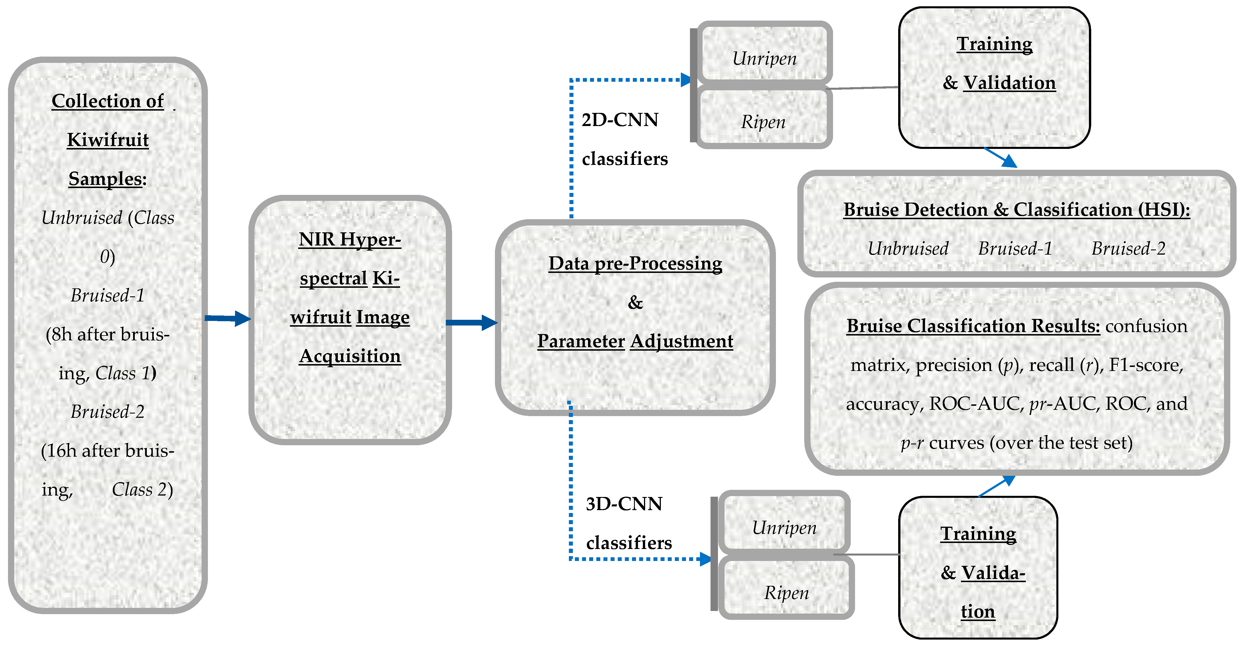
The schematic workflow system methodology for detecting bruised kiwifruit is given in Figure 1. The methodology is founded on the basis of both 2D-CNN and 3D-CNN network architectures.
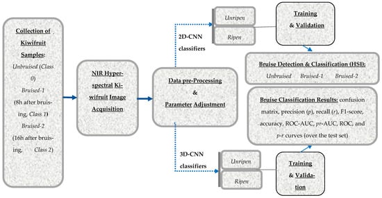
Figure 1.
Workflow diagram of the proposed bruise detection and classification system in both unripe and ripe kiwifruit: Unbruised (Class 0), Bruised-1 (8 h after bruising, Class 1), and Bruised-2 (16 h after bruising, Class 2) for both 2D-CNN and 3D-CNN classifier networks are depicted in the graph. The classification performance results include precision , recall , F1-score, accuracy (CCR), ROC-AUC, pr-AP, ROC, and p-r curves. 2D: two-dimensional, 3D: three-dimensional, ROC: receiver operating characteristic, CNN: convolutional neural network, pr: precision–recall, AP: average precision, HSI: hyperspectral imaging, NIR: near-infrared.
2.1. Collecting the Samples
A total of 420 Hayward kiwifruit were collected randomly from four gardens located in Ramsar, Iran (36.9268° N, 50.6431° E). The samples were handpicked in two ripening categories: unripe (one week before the optimal ripening stage) and ripe (optimal ripening stage). In fact, 210 kiwis were considered for each category in three classes i.e., undamaged (Unbruised or Class 0), 8 h after bruising (Bruised-1 or Class 1), and 16 h after bruising (Bruised-2 or Class 2). Since two samples of bruised kiwi were destroyed, to equalize the number of samples in each class, 68 samples were considered for each class (408 samples in total). The samples were considered separately in each class in order to increase the reliability of the trained model.
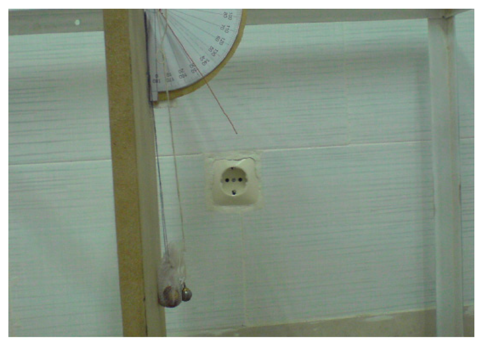
Each fruit was packed in foam and was located inside one-rowed boxes, so mechanical damage was minimized. Hyperspectral images of the healthy samples were acquired. To provide artificially induced bruising damage to the fruit, a metal object (bullet, weight = 32 g) was used (see Figure 2). The fruit was placed inside a textile net and hung as shown in Figure 2. The metal ball was released following a free fall pendulous path at a determined angle to hit the fruit in its middle point approx. Based on previous test and error essays of different angular (and distance) ball releases, an angle of 30 degrees from the vertical line was chosen to induce fruit bruising (see Figure 2). Hyperspectral imaging of bruised fruit was then captured and labeled as Bruised-1 (HSI images taken 8 h after induced bruising) and hyperspectral imaged again, labeled as Bruised-2 (HSI images taken 16 h after induced bruising).
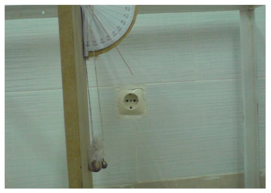
Figure 2.
The setup used to induce physical bruises on the kiwifruit samples of either Bruised-1 (8 h after hit) or Bruised-2 (16 h after hit): a 32 g metal bulled was used as free fall to hit and induce bruise damage on the fruit under consideration, from an angle of 30° measured w.r.t. the vertical direction.
2.2. Setup and Hardware Used to Collect the Spectral-Spatial Hyperspectral Imaging (HSI) Data
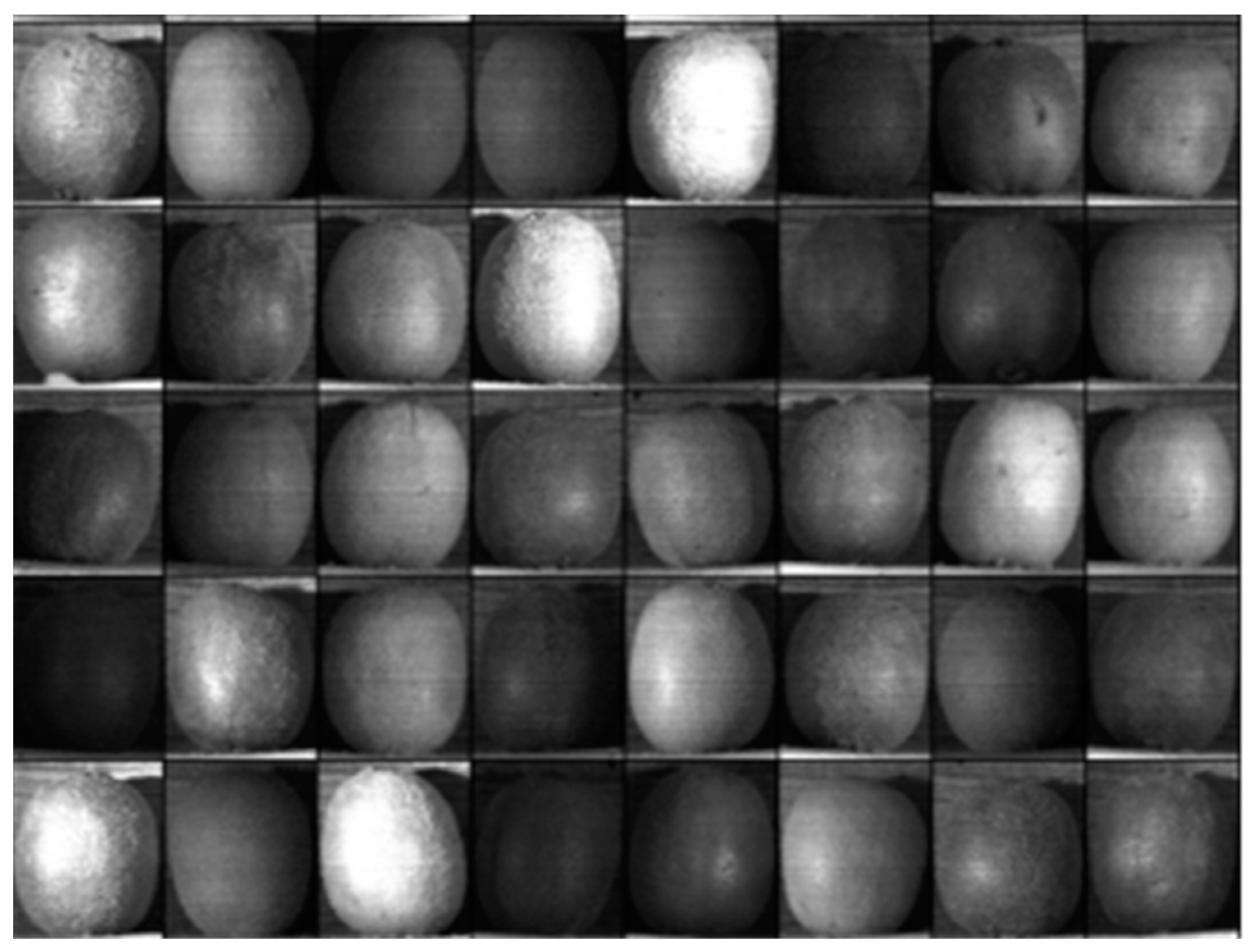
AN NIR hyperspectral imaging (HSI) camera with software and a built-in scanner (Noor Imen Tajhiz Co.; https://hyperspectralimaging.ir/ (accessed on 11 August 2023), made in Kashan, Iran) at the range of 400–1100 nm with a spectral resolution of 2.5 nm was used to acquire the hyperspectral fruit images (Figure 3). To prevent ambient light reflections and distortions, the HSI camera was set inside an illumination chamber equipped with two halogen lamps (20 watts each) as the light source. It should be noted that the images at the beginning and end of the spectral range of the HSI camera were corrupted with a lot of noise; therefore, those wavelength spectral extreme bands were discarded during the pre-processing phase. The remainder of the HSI images were resized by removing the background, c.f. Figure 3.

Figure 3.
Various examples of kiwifruit hyperspectral (HSI) input images depicted at various wavelength values (frequency bands).
2.3. The Input Dataset Samples: Train, Test, and Validation Disjoint Sets
The input HSI image dataset was randomly split into three disjoint subsets: train, test, and validation sets, with portions of 60%, 25%, and 15% of total samples, respectively. Table 1 gives the number of samples in the dataset for each class as well as for each disjoint subset (train, test, and validation). By disjoint sets, we mean sets that do not share a single element in common. It is worth noting that the 2D-CNNs did not need data augmentation because the number of samples was sufficient, i.e., an image of each individual wavelength (174 frequency bands in total) multiplied by 68 (the number of kiwifruit samples in each class) produced a total of 11,832 images.

Table 1.
Number of input HSI image samples in the dataset: train/test/validation disjoint subsets. The 2D-CNN numbers of the input samples are those of the 3D-CNN multiplied by 174 (HSI frequency bands); thus, the 2D-CNN did not need data augmentation. Unbruised, Bruised-1, and Bruised-2 kiwifruit categories.
2.4. Convolutional Neural Network (CNN) Classifiers: 2D-CNN and 3D-CNN
2.4.1. 2D-Convolutional Neural Network (2D-CNN)
A two-dimensional (2D) convolutional layer (see Figure 4) computes the dot product of the network weights and the input data (image) by moving the convolutional filter kernel mask “sliding” along the vertical and horizontal direction of the 2D input data (image) computing the convolution operation of the input data by adding a certain bias [28].

Figure 4.
A simple diagram of the structure of a two-dimensional convolution neural network (2D-CNN) with two convolution layers.
2.4.2. 3D-Convolutional Neural Network (3D-CNN)
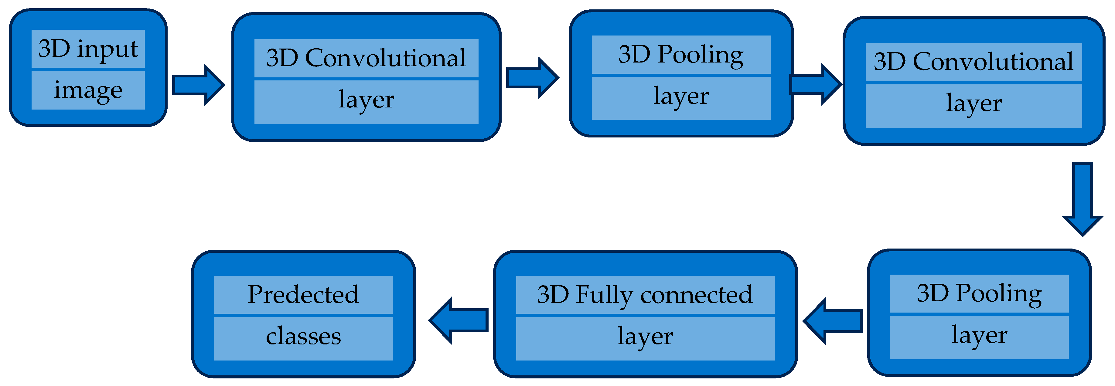
In a 3D-CNN, a three-dimensional (3D) filter kernel (see Figure 5) slides in the three “spatial” directions: a hyperspectral image cube comprises two spatial and one spectral (wavelength) coordinate(s). On the other side, a 2D-CNN can only slide in two spatial (image) dimensions. In a 2D-CNN, the same weights for the whole multiple frequency wavelength channels (bands) are used and result in a single 2D image, but a 3D volume (cube) is produced in 3D convolutions, leading to the preservation of the frequential information of the frame stack [29].
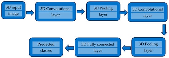
Figure 5.
A simple diagram of a 3D convolutional neural network (3D-CNN) structure with two convolutional layers.
2.5. Models of CNN Neural Architectures
2.5.1. PreActResNet Architecture
The pre-activation version of ResNet, known as PreActResNet, is a variation of the original ResNet architecture that improves the performance of the original ResNet network by placing an activation layer before the weight layer [30].
2.5.2. GoogLeNet Architecture
The GoogLeNet architecture includes 22 deep layers with 27 pooling layers. There are 9 inception modules placed in a queue for subsequent processing where the end ones are connected to the global average pooling layer [31].
2.6. Performance Classification Indices: Confusion Matrix, Precision , Recall , Accuracy (CCR), F1-Score, Receiver Operating Characteristic (ROC), and pr Curves
To evaluate the different classifiers’ architecture performance, various well-known metric criteria are defined and computed, including confusion matrix, precision (), recall () or a.k.a. as sensitivity, accuracy, F1-score, receiver operating characteristic (ROC), and precision–recall () curves. Definitions for any binary classifier follow next:
where TP is the true positive, TN is the true negative, FP is the false positive, and FN is the false negative cases. In addition, the area under the curve (AUC) values for and ROC curves, -AP, and ROC-AUC will also be computed as an additional classification performance metric.
Whenever the FP and FN costs are unknown or may differ a lot from one another, one does not have an optimal working point of the classifier and needs to evaluate the classification performance for a slowly varying output classifier decision threshold. Critical classification tasks are a good example: in computer-aided medical diagnosis, FN (saying no cancer and thus not starting treatment when in fact cancer exists) is often much worse than FP (upsetting a patient saying cancer exists while in a later phase test, it will be confirmed that no such cancer is present), while on the contrary in war, an FP (eliminating a non-enemy, i.e., eliminating a civilian or even your own troops) is judged as worse than an FN (not eliminating an enemy, given you are not sure). In those extreme cases and many more where the costs associated with FP and FN misclassifications are simply unknown, it is not enough with a single working point (output decision threshold), and one needs to evaluate the classifier for several output threshold values. That is when the ROC and precision–recall curves are very useful in evaluating classifier performance:
- (a)
- The ROC curve computes the plot over the whole range by slowly varying the classifier output detection threshold. All ROC curves vary from to the points in the plane when varying the output classifier threshold, but the difference between a good and a bad classifier is the area under the ROC curve (AUC) that the classifier is able to accumulate in the plane, called the ROC-AUC.
- (b)
- The precision–recall () curve plots the plot over the whole range, slowly varying the classifier detection threshold. All curves vary from to the points in the plane while varying the output classifier threshold.
A classifier with an ROC − AUC = 0.5 is a totally useless classifier, equivalent to the simple toss of a coin, while on the contrary, a classifier which in the limit has an is an optimal classifier, tending to the optimal plane point at in the top-left corner of the ROC plot, making no single misclassification only whenever AUC = 1, and the higher the AUC values, the better classification one has. If any classifier had an (making more errors than hits), then the opposite decision classifier would be taken, with it always having , thus making more hits than errors, on average.
3. Results
3.1. Bruised Area Induced in the Hyperspectral Fruit Images
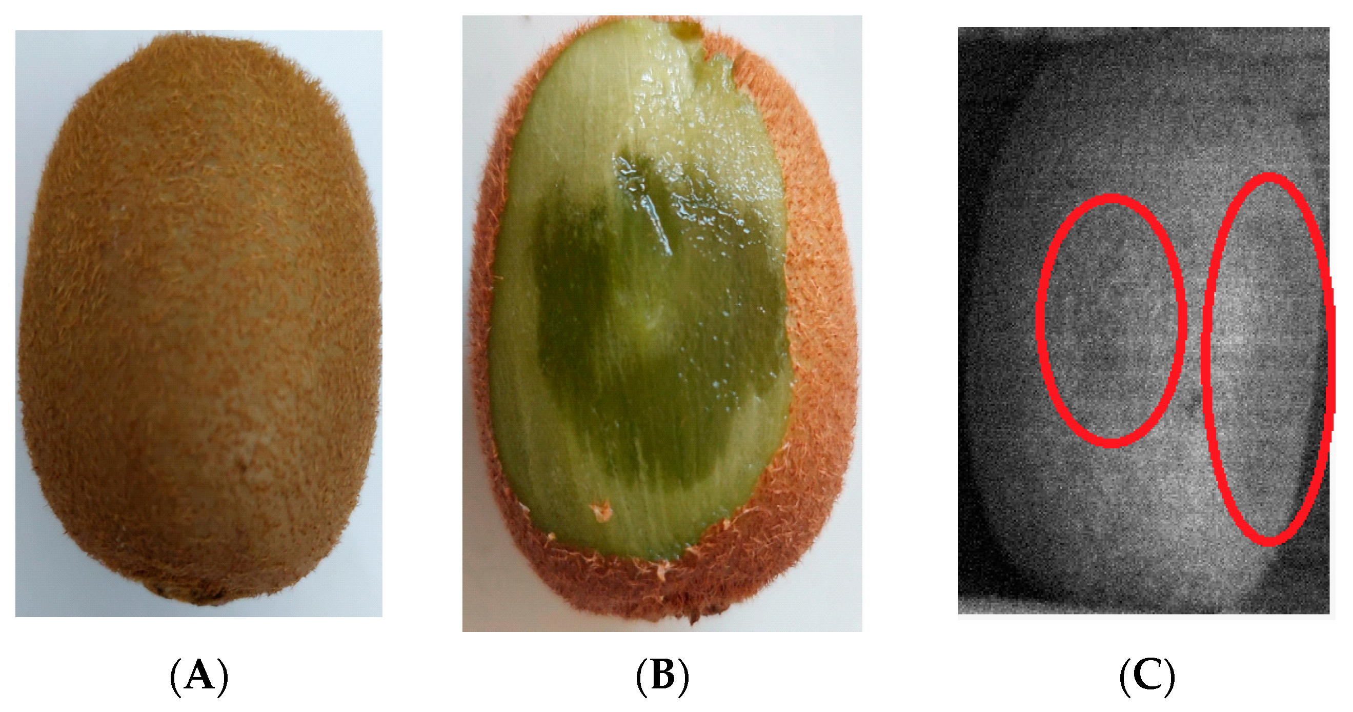
Since the skin of kiwifruit does not discolor in the early hours after bruising, visual detection of bruised fruit is a major challenge here. Figure 6 gives an example of a hyperspectral image of a bruised fruit in the early hours after damage was produced. As observable in Figure 6C, bruised areas are seen slightly darker in the HSI image, which validates the ability of the hyperspectral imaging technology to be used to properly detect bruised areas in fruit.
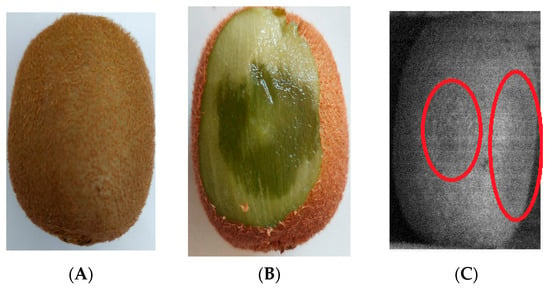
Figure 6.
An example of an bruised kiwifruit image, belonging to the Bruised-2 fruit class: (A) image captured by an ordinary visible (Vis) range RGB CCD camera, where the bruised area is hidden in the image; (B) the bruised area after peeling the fruit appears apparent on the same Vis CCD camera; and (C) the bruised area captured by the hyperspectral camera at a near-infrared wavelength (815 nm) before peeling the fruit, with the bruised fruit area shown to be slightly darker and highlighted inside two red circles in the image.
3.2. 3D-CNN Architecture Based on the PreActResNet Model
3.2.1. Classification Performance of the 3D-CNN Architecture Based on the PreActResNet Network
The performance of the 3D-CNN architecture based on the PreActResNet model was evaluated with the computation of the confusion matrix (Figure 7) and classification performance indices with recall, precision, and F1-score (Table 2). According to Figure 7 and Table 2, it was concluded that the detection of bruising in the ripe fruit could be more challenging because when kiwifruit is mature, its sensitivity to bruising increases, and it becomes more difficult to identify damaged tissue due to lower image contrast.
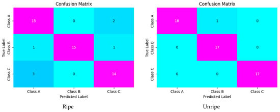
Figure 7.
Confusion matrices of the 3D-CNN architecture based on the PreActResNet model: classA: Unbruised, class B: Bruised-1, and class C: Bruised-2.

Table 2.
Classifier performance of the 3D-CNN architecture based on the PreActResNet model: Unbruised, Bruised-1, and Bruised-2, and unripe and ripe fruit cases. AP: average precision.
Precision () is computed by dividing the true positives by anything that was predicted as a positive, see (1). Recall () (or true positive rate, TPR) is computed by dividing the true positives by anything that should have been predicted as positive, see (1). In other words, recall () illustrates whether samples can be properly found out by the algorithm or not, while precision () illustrates how many correct classifications can be achieved. The F1-score is computed as the harmonic mean of a system’s precision, and recall values together: .
3.2.2. Precision–Recall (pr) and ROC Curves of the 3D-CNN Architecture Based on the PreActResNet Model
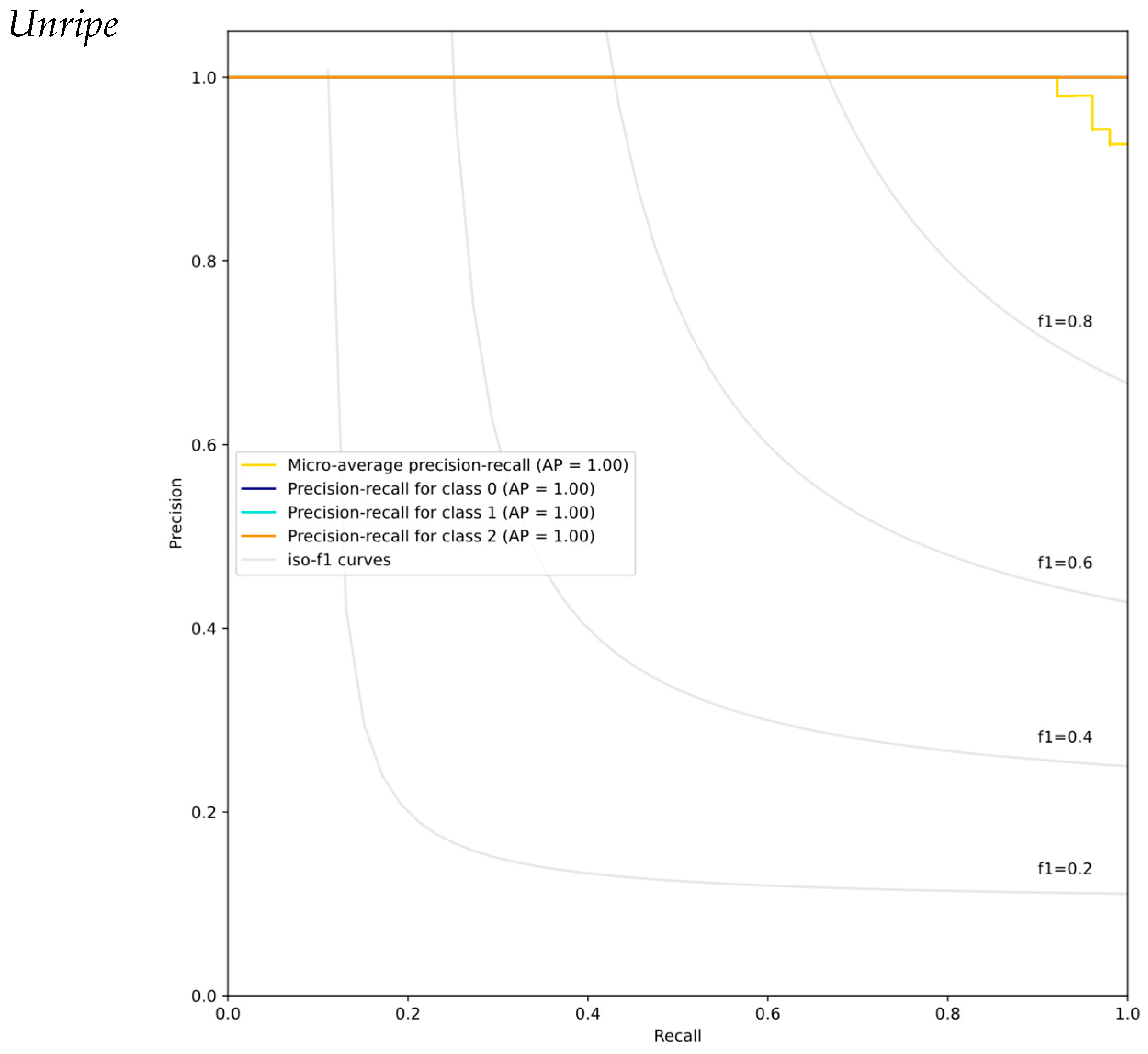
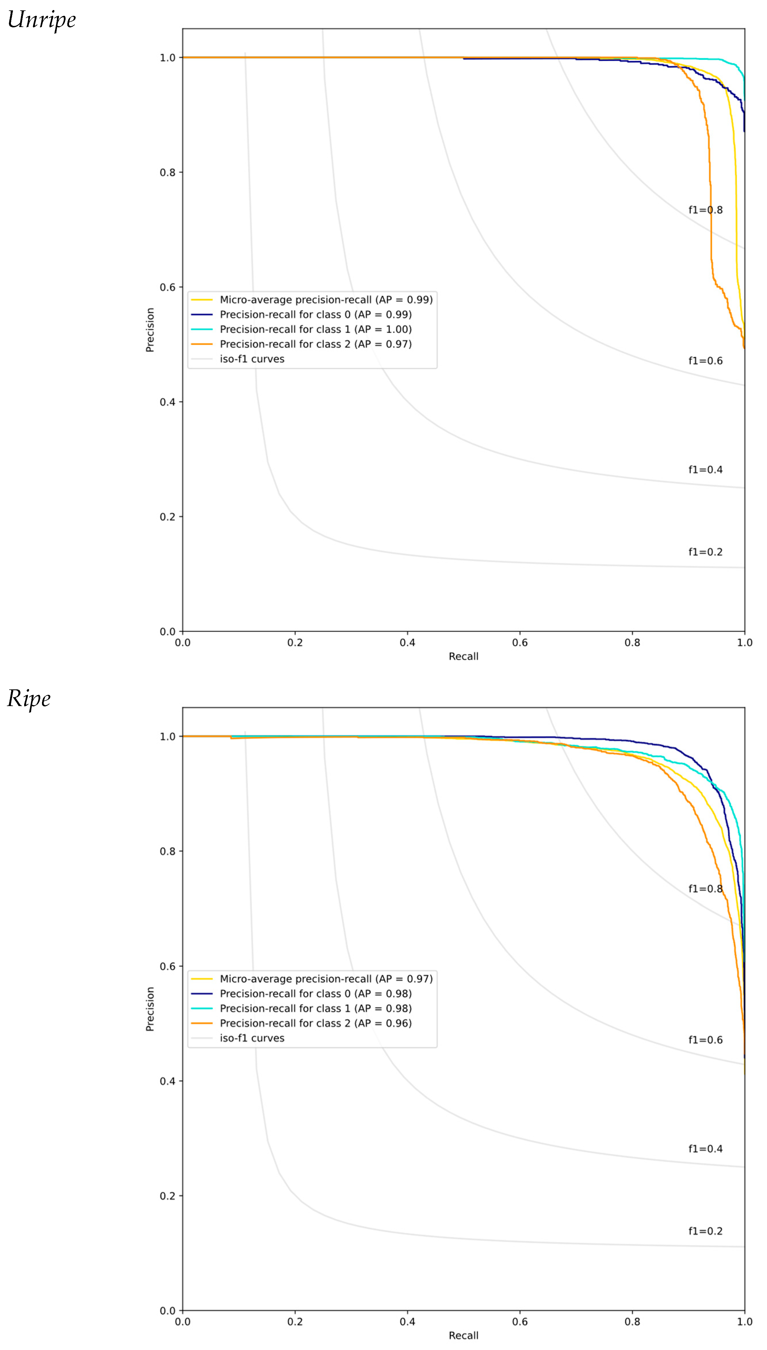
The performance of the classifier was evaluated by a criterion called average precision (AP). Figure 5 shows precision–recall and -AP criteria values for the overall ternary classification problem, micro-average. Figure 8 shows precision–recall and -AP values per each of the three classes. The AP of classes in the unripe fruit case (100%) is higher than that for ripe fruit, implying that the detection of bruising in the unripe fruit is more successful than in the ripe counterpart.
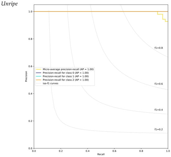
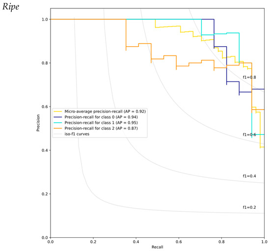
Figure 8.
Precision–recall curves and -AP values per each class for the 3D-CNN architecture based on the PreActResNet model: Unbruised (Class 0), Bruised-1 (Class 1), and Bruised-2 (Class 2), and unripe and ripe fruit cases. AP: average precision. Constant F1-score curves are also depicted in the figure.
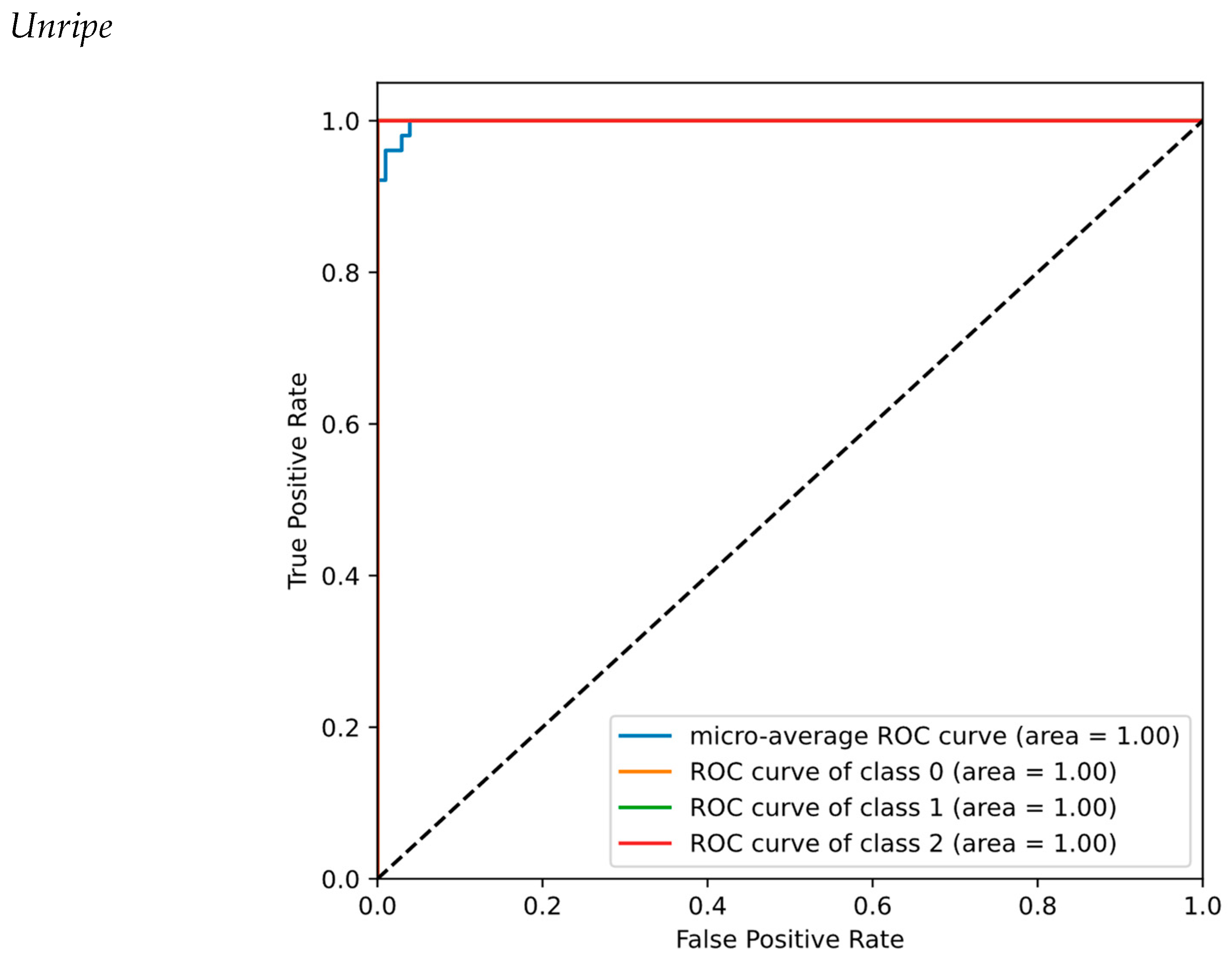
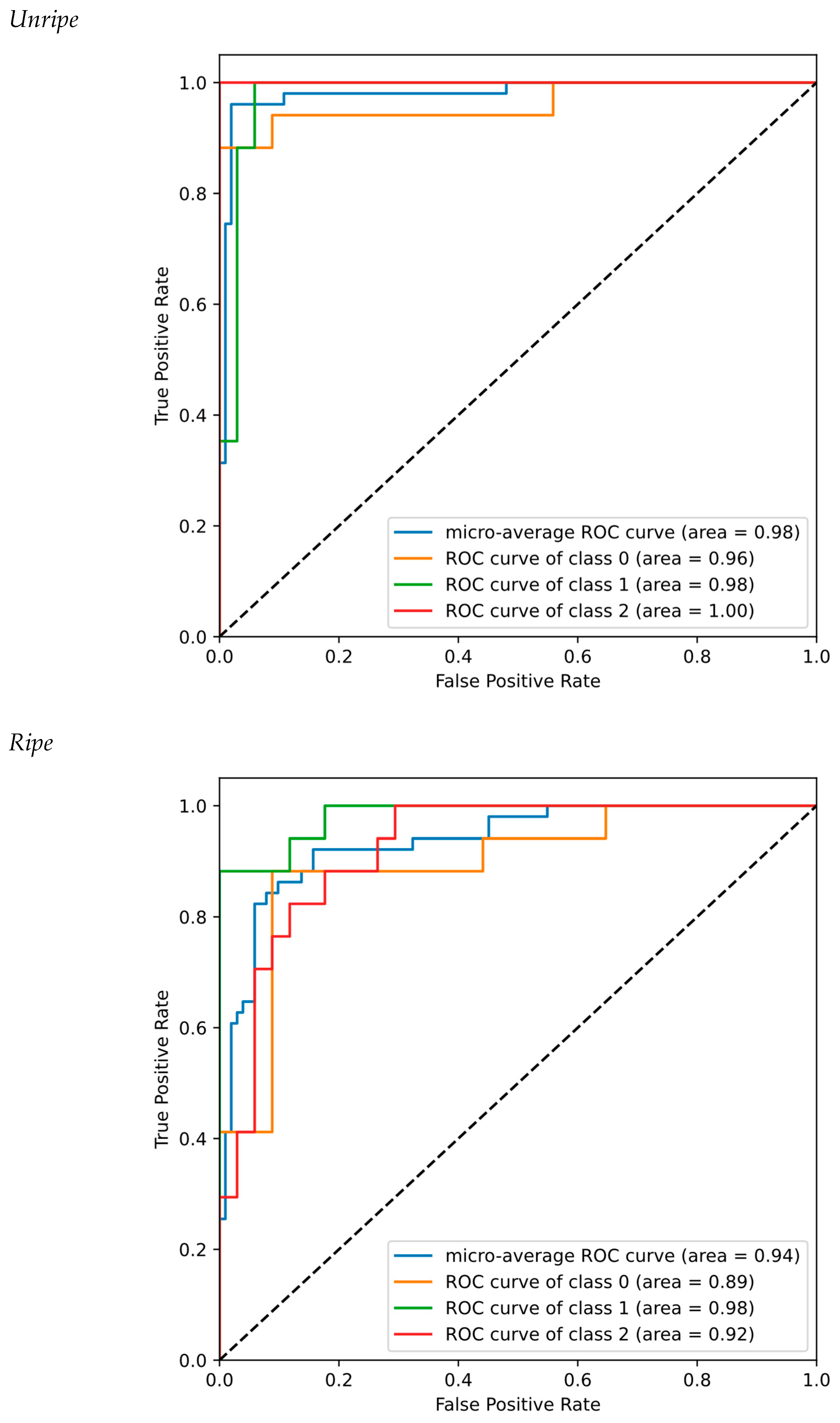
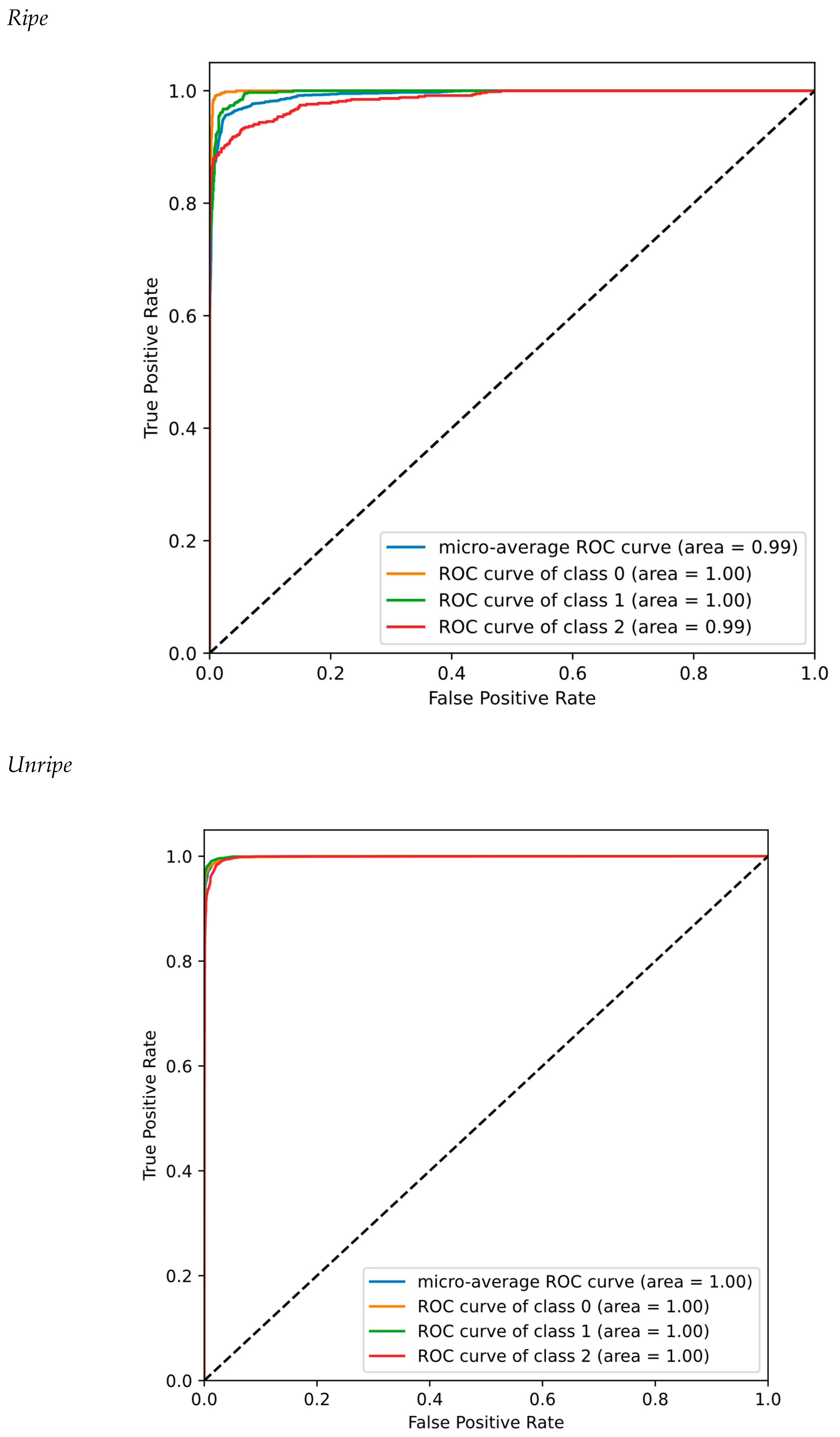
The receiver operating characteristic (ROC) curve is one of the methods most often used to evaluate the performance of binary classification. The efficiency of a binary classifier is usually measured by sensitivity and specificity values. In the ROC chart, both criteria are combined and displayed as a curve in the {1—specificity, sensitivity} plane or equivalently in the (FPR, TPR) plane, where FPR stands for false positive rate. The closer the ROC curve is to the top left corner of the chart , the better the performance of the classifier is (Figure 9).
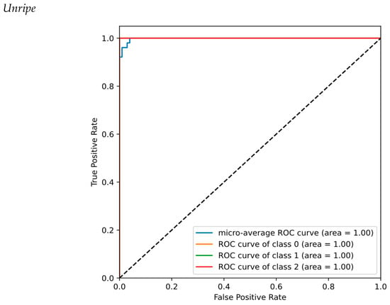
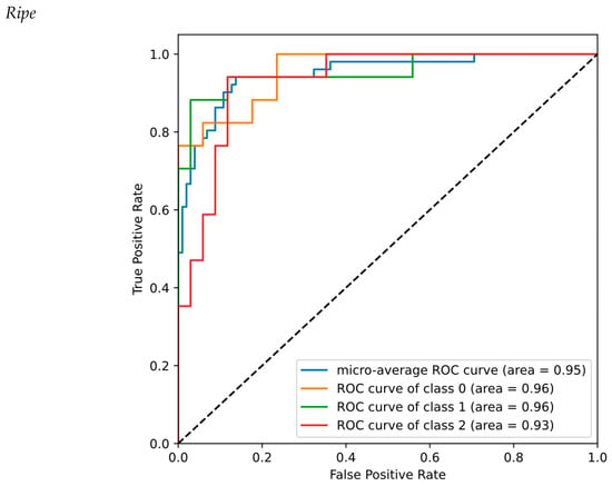
Figure 9.
ROC curves and RO-AUC values for the 3D-CNN architecture based on the PreActResNet model: Unbruised (Class 0), Bruised-1 (Class 1), and Bruised-2 (Class 2), and unripe and ripe fruit cases.
3.3. 3D-CNN Architecture Based on the GoogLeNet Model
3.3.1. Classification Performance of the 3D-CNN Architecture Based on the GoogLeNet Model
Figure 10 gives the performance of the 3D-CNN classifier architecture (GoogLeNet model) based on the confusion matrix. Other performance criteria like precision, recall, and F1-score are also given in Table 3. The true positive rate (TPR) of each class was reflected as the recall criteria. A recall value of 100% means that no samples of other classes are misclassified in the given class.
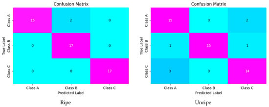
Figure 10.
Confusion matrices of the 3D-CNN architecture based on the GoogLeNet model: classA: Unbruised, class B: Bruised-1, and class C: Bruised-2.

Table 3.
Classification performance of the 3D-CNN architecture based on the GoogLeNet model: Unbruised, Bruised-1 and Bruised-2, and unripe and ripe fruit cases.
Precision is computed by dividing the true positives by anything that was predicted as a positive, see (1). The F1-score is the harmonic mean of a system’s precision and recall values, see (1). As observed from Table 4 and Table 5, the unripe category behaves better than ripe in terms of both confusion matrices and classification performance indices.

Table 4.
Classification performance of the 2D-CNN architecture based on the PreActResNet model: Unbruised, Bruised-1 and Bruised-2, and unripe, and ripe fruit cases.

Table 5.
Classifier performance of the 2D-CNN architecture based on the GoogLeNet model: Unbruised, Bruised-1 and Bruised-2, and unripe and ripe fruit cases.
3.3.2. Precision–Recall and ROC Curves of the 3D-CNN Architecture Based on the GoogLeNet Model
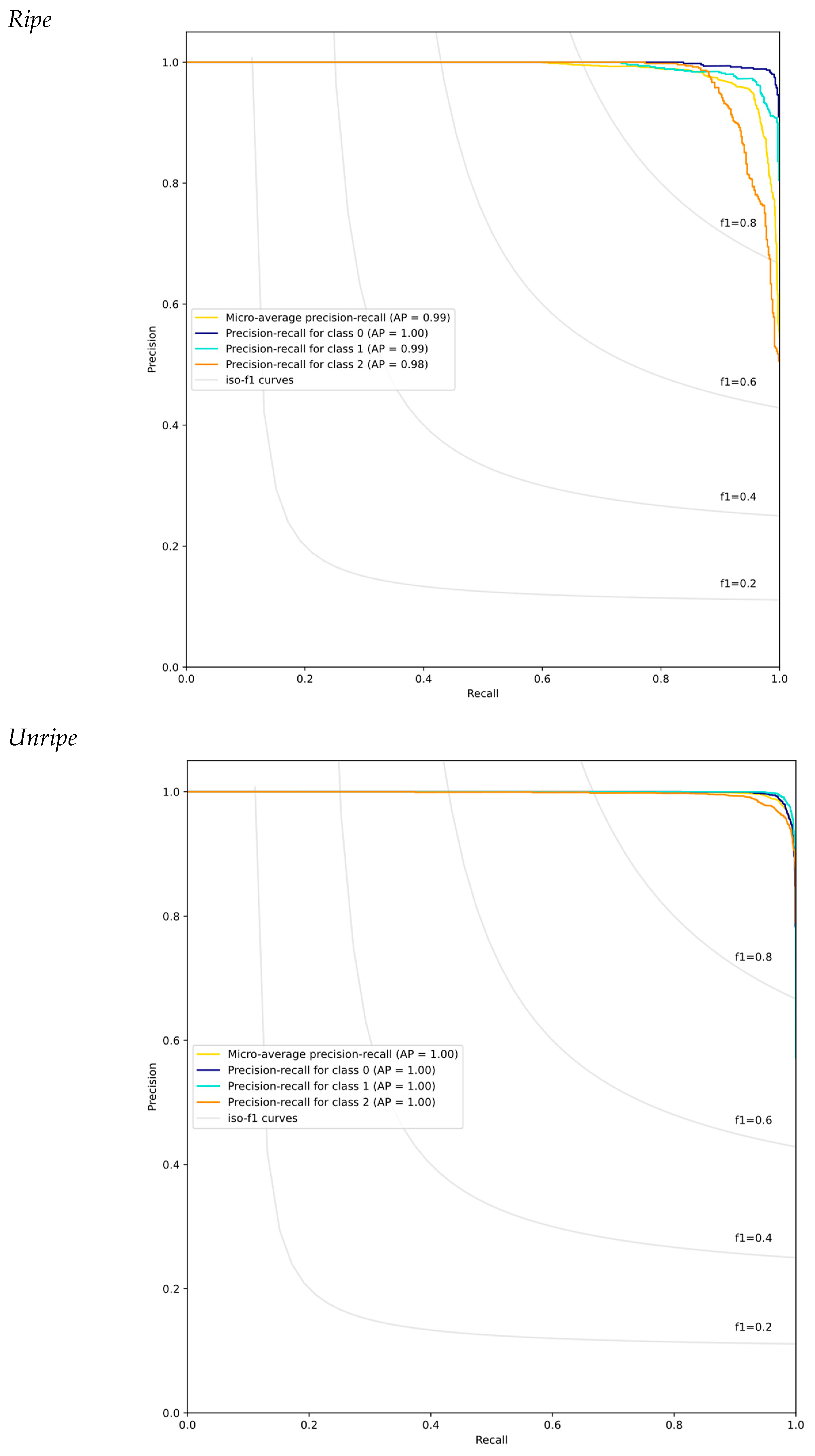
The average precision (AP) or -AP averaged over the three classes (micro-average) for the unripe stage is higher than the ripe stage, implying that the algorithm was more successful in bruise detection of the unripe kiwi (Figure 11). Moreover, the ROC curve for the unripe case is closer to the optimal working point at the top-left chart corner (Figure 12), where . In this classifier model (3D-CNN GoogLeNet), the performance of the unripe fruit category is substantially superior to that of its ripe counterpart, consistently.
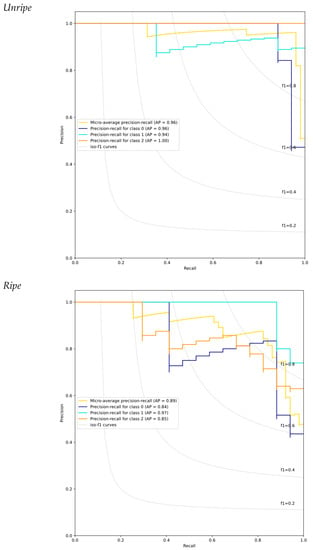
Figure 11.
Precision–recall curves and -AP values per each class for the 3D-CNN architecture based on the GoogLeNet model: Unbruised (Class 0), Bruised-1 (Class 1), and Bruised-2 (Class 2), and unripe and ripe fruit cases. AP: average precision. Constant F1-score curves are also depicted in the figure.
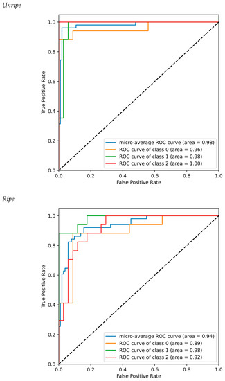
Figure 12.
ROC curves and ROC-AUC values for the 3D-CNN architecture based on the GoogLeNet classifier model: Unbruised (Class 0), Bruised-1 (Class 1), and Bruised-2 (Class 2), and unripe and ripe fruit cases.
3.4. 2D-CNN Architecture Based on the PreActResNet Model
3.4.1. Classification Performance of the 2D-CNN Architecture Based on the PreActResNet Model
Figure 13 gives the performance of the 2D-CNN architecture (PreActResNet model) based on the confusion matrix. Other evaluating criteria including precision, recall, and F1-score are given in Table 4. In both tables it is seen that the performance of the classification model is very remarkable, being slightly over those of the 3D-CNN GoogLeNet counterpart. Again, the substantially superior performance for the unripe case as compared to the ripe case was observed, also with a different classifier architecture, the 2D-CNN PreActResNet.
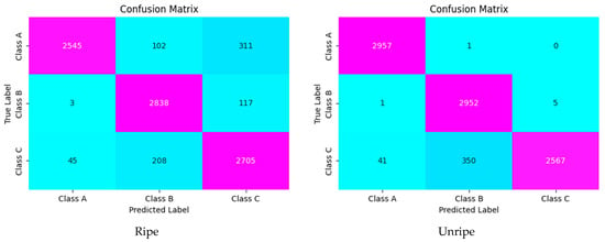
Figure 13.
Confusion matrices of the 2D-CNN architecture based on the PreActResNet model: classA: Unbruised, class B: Bruised-1, and class C: Bruised-2.
3.4.2. Precision–Recall and ROC Curves of the 3D-CNN Architecture Based on the PreActResNet Model
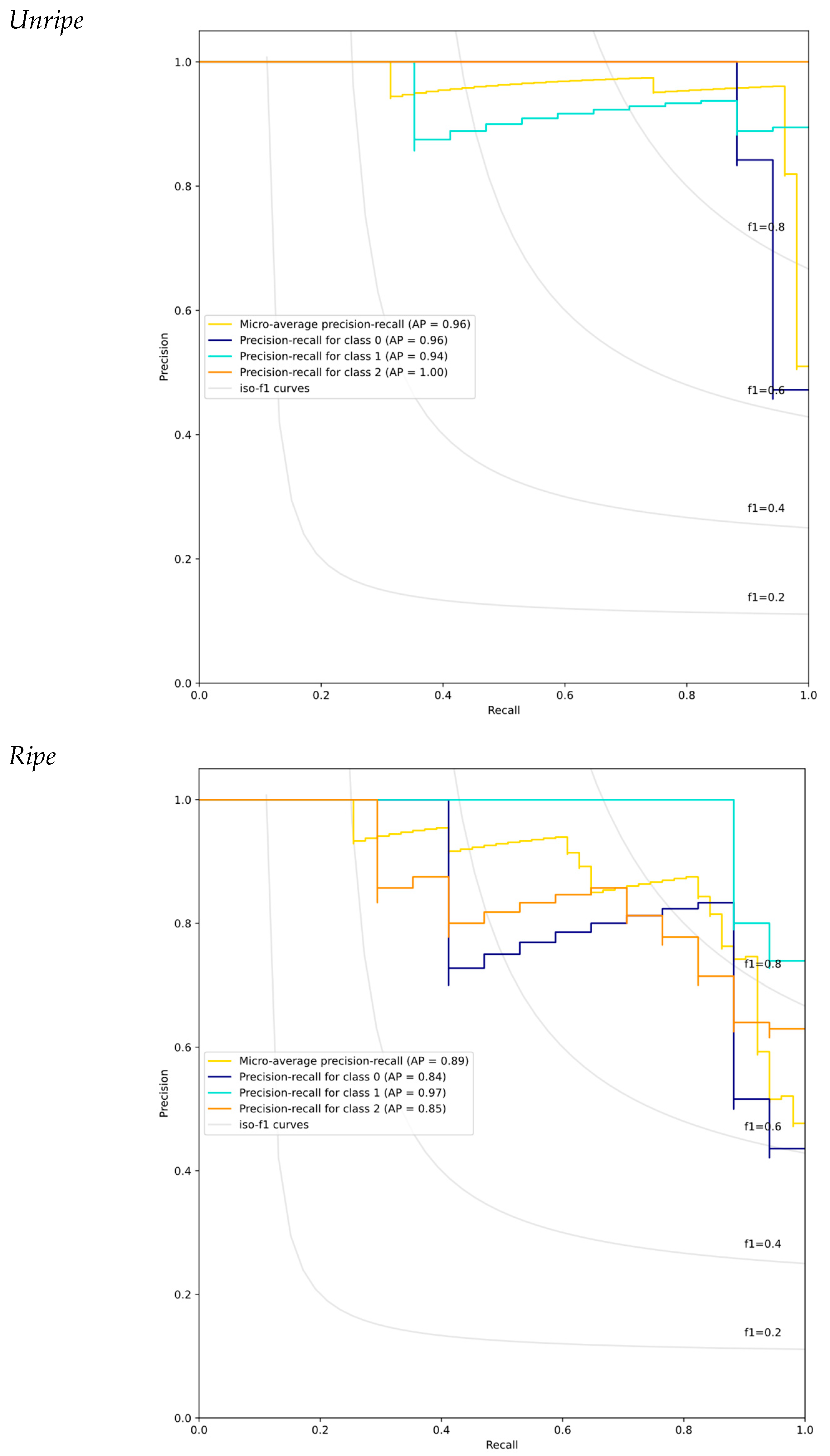
Once more, the average precision (AP) or -AP values averaged for the three classes (micro-average) for the unripe stage is higher than the ripe counterpart, implying that the algorithm was more successful in bruise detection of unripe kiwifruit (Figure 14), thus reaching closer to the optimal pr curve working point in the top-right corner of the plot, where: . Moreover, the ROC curve for the unripe case is also closer to the optimal top-left corner point (Figure 15), where .
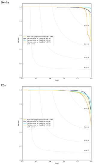
Figure 14.
Precision–recall curves and -AP values per each class for the 2D-CNN architecture based on the PreActResNet classification model: Unbruised (Class 0), Bruised-1 (Class 1), and Bruised-2 (Class 2), and unripe and ripe fruit cases. AP: average precision. Constant F1-score curves are also depicted in the figure.
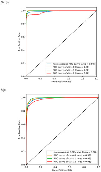
Figure 15.
ROC curves and ROC-AUC values computed for the 2D-CNN architecture based on the PreActResNet classification model: Unbruised (Class 0), Bruised-1 (Class 1), and Bruised-2 (Class 2), and unripe and ripe fruit cases.
3.5. 2D-CNN Architecture Based on the GoogLeNet Model
3.5.1. Classifier Performance of the 2D-CNN Architecture with the GoogLeNet Model
Figure 16 gives the performance of the 2D-CNN architecture (GoogLeNet model) based on the confusion matrix. Additional evaluation criteria including precision, recall, and F1-score are given in Table 5. All parameters are above 93% for unripe and ripe kiwi, implying that the model was successful in bruise detection.
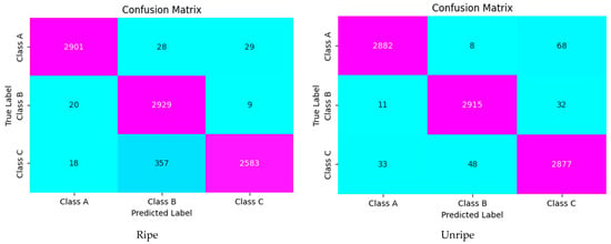
Figure 16.
Confusion matrices of the 2D-CNN architecture based on the GoogLeNet model: classA: Unbruised, class B: Bruised-1, and class C: Bruised-2.
3.5.2. Precision–Recall and ROC Curves of the 2D-CNN Architecture Based on the GoogLeNet Classifier Model
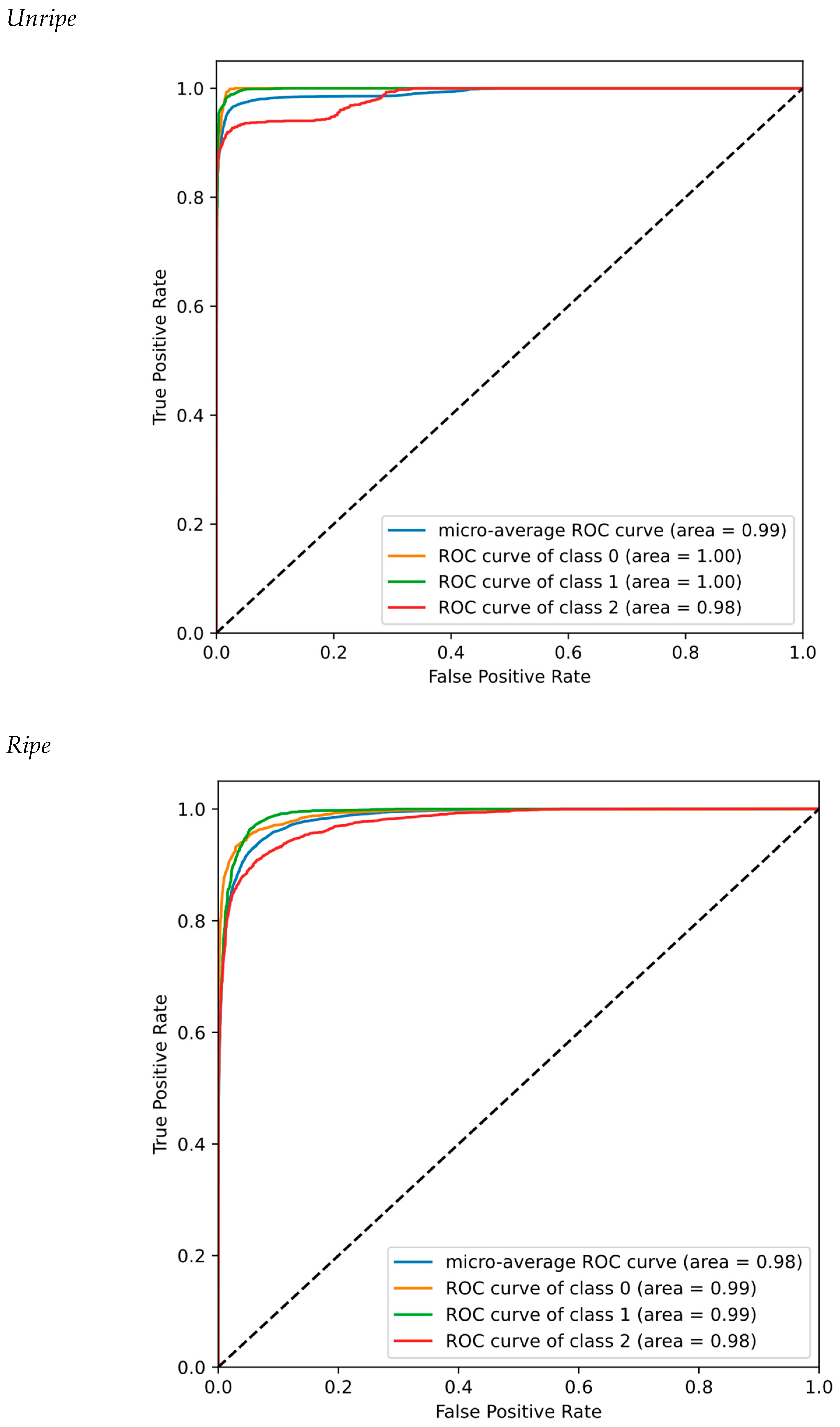
The average precision (AP) or -AP values computed for the unripe stage is higher than ripe stage, which means that the system was more successful in the bruise detection of unripe kiwi as compared to ripe kiwi (Figure 17), reaching the optimal plane working point in the top-right corner, where . Moreover, the ROC curve for the unripe case is closer to the optimal top-left chart corner (Figure 18), where , as compared to its ripe fruit case counterpart, for the 2D-CNN GoogLeNet classifier.
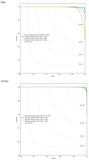
Figure 17.
Precision–Recall curves and pr-AP values computed per each class for the 2D-CNN architecture based on the GoogLeNet classifier: Unbruised (Class 0), Bruised-1 (Class 1), and Bruised-2 (Class 2), and unripe, and ripe fruit cases. AP: average precision. Constant F1-score curves are also depicted in the figure.
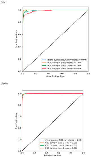
Figure 18.
ROC curves and ROC-AUC values computed for the 2D-CNN architecture based on the GoogLeNet classifier: Unbruised (Class 0), Bruised-1 (Class 1), and Bruised-2 (Class 2), and unripe and ripe fruit cases.
3.6. Comparison between the Results of Related Studies and Those of the Proposed Method
Next, in Table 6 we compare the classification performance results here shown with some from the literature. Please note both the fruit type and dataset used are different, thus no direct comparison is possible.

Table 6.
Comparison of the results of related fruit classification studies with the present paper. The correct classification rates (CCRs) values are in a similar range.
3.7. Future Studies
This work presents a significant advancement in the field of post-harvest bruising detection. It lays a solid foundation for future studies on similar topics and encourages the exploration of hyperspectral imaging and advanced machine learning models in bruise detection across a broader range of fruits and vegetables. Given the promising results obtained in this study, several areas of research can be suggested for the future. One of them is to investigate the model’s ability to detect natural bruises or to compare artificially induced bruises with natural ones, which could validate the model’s robustness in real-world scenarios. Also, with an erosion study in future research, a better understanding of the performance of the developed models can be obtained because, in such a study, the contribution of each component of the model can be understood.
4. Conclusions
The early and non-destructive detection of bruising in kiwifruit was conducted here by processing local spatio-spectral NIR hyperspectral imaging data with 2D-CNN and 3D-CNN convolutional neural network classifiers, with the main results summarized next to conclude:
- As observed comparing both Vis (RGB) and NIR hyperspectral kiwifruit images, bruised areas are seen slightly darker in the HSI images, which validates the ability of the HSI imaging technology to be used in the early detection of bruised areas in fruit.
- The early, automatic, and non-destructive detection of the bruising area on HSI imaging was more accurate in the case of unripe fruit as compared to the ripe fruit case, with an exception made for the 2D-CNN GoogLeNet classifier which showed the opposite behavior, with a consistent difference and for all three kiwifruit classes. An explanation of this fact might be the higher contrast of the color change after bruising of the fruit flesh in unripe fruit as compared to ripe fruit; despite this, the hypothesis needs to be further investigated for proper validation.
- The accuracy of the 2D and 3D models is higher than 95% for the unripe samples. The reason goes back to the physiological issues of Kiwi. In fact, in the unripe samples, due to the firmness of the fruit, discoloration of the bruise is more obvious than in the ripe ones.
- Another important point is the superiority of the 2D-CNN classifier compared to 3D models, which can be due to the following: (1) the complexity of 2D-CNN is lower because it examines information only in the spatial dimension, and as a result, it achieves more accuracy in the classification of hyperspectral images, and (2) due to the focus of the 2D-CNN on spatial features, the extraction of spatial features from hyperspectral images is better, so the accuracy increases
- According to the comparison with previous research, the correct classification rate (CCR) is comparable, and it can be stated that the proposed methods provide promising results in the early identification of kiwifruit.
- It is common among gardeners to harvest kiwifruit a little too early because it is prone to bruising during transportation. Since the results of the proposed classifiers were more promising in identifying bruise symptoms for hard status than the soft mode, the alignment of the results with gardeners’ actions can therefore be applicable to kiwi grading.
Author Contributions
Conceptualization, R.P. and S.E.; methodology, S.S.; software, S.S.; validation, J.I.A. and M.H.R.; investigation, R.P.; data curation, S.E.; writing—original draft preparation, R.P.; writing—review and editing, J.I.A.; supervision, R.P.; project administration R.P.; funding acquisition, S.E. All authors have read and agreed to the published version of the manuscript.
Funding
This work was funded in part under grant number PID2021-122210OB-I00 from Proyectos de Generacion del Conocimiento 2021, Investigacion Orientada, Plan Estatal de Investigacion Cientifica, Tecnica y de Innovacion, 2021–2023, Ministry for Science, Innovation and Universities, Agencia Estatal de Investigacion (AEI), Spain, and Fondo Europeo de Desarrollo Regional, European Union (E.U.).
Data Availability Statement
The data that support the findings of this study are available upon request from the corresponding author. The data are not publicly available due to privacy or ethical restrictions.
Acknowledgments
The authors acknowledge Proyectos de Generacion del Conocimiento 2021 (grant number PID2021-122210OB-I00), Investigacion Orientada, Plan Estatal de Investigacion Cientifica, Tecnica y de Innovacion, 2021–2023, Ministry for Science, Innovation and Universities, Agencia Estatal de Investigacion (AEI), Spain, and Fondo Europeo de Desarrollo Regional, European Union (E.U.).
Conflicts of Interest
The authors declare no conflict of interest.
References
- Li, Z.; Liu, J.; Li, P. Relationship between mechanical property and damage of tomato during robot harvesting. Trans. Chin. Soc. Agric. Eng. 2010, 26, 112–116. [Google Scholar] [CrossRef]
- Li, Z.; Thomas, C. Quantitative evaluation of mechanical damage to fresh fruits. Trends Food Sci. Technol. 2014, 35, 138–150. [Google Scholar] [CrossRef]
- Soleimani, B.; Ahmadi, E. Evaluation and analysis of vibration during fruit transport as a function of road conditions, suspension system and travel speeds. Eng. Agric. Environ. Food 2015, 8, 26–32. [Google Scholar] [CrossRef]
- Al-Dairi, M.; Pathare, P.B.; Al-Yahyai, R.; Opara, U.L. Mechanical damage of fresh produce in postharvest transportation: Current status and future prospects. Trends Food Sci. Technol. 2022, 124, 195–207. [Google Scholar] [CrossRef]
- Sun, Z.; Hu, D.; Xie, L.; Ying, Y. Detection of early stage bruise in apples using optical property mapping. Comput. Electron. Agric. 2022, 194, 106725. [Google Scholar] [CrossRef]
- Lu, Y.; Lu, R.; Zhang, Z. Detection of subsurface bruising in fresh pickling cucumbers using structured-illumination reflectance imaging. Postharvest Biol. Technol. 2021, 180, 111624. [Google Scholar] [CrossRef]
- Opara, U.L.; Pathare, P.B. Bruise damage measurement and analysis of fresh horticultural produce—A review. Postharvest Biol. Technol. 2014, 91, 9–24. [Google Scholar] [CrossRef]
- Ragulskis, K.; Ragulskis, L. Dynamics of a single mass vibrating system impacting into a deformable support. Math. Model. Eng. 2020, 6, 66–78. [Google Scholar] [CrossRef]
- Fu, H.; Karkee, M.; He, L.; Duan, J.; Li, J.; Zhang, Q. Bruise Patterns of Fresh Market Apples Caused by Fruit-to-Fruit Impact. Agronomy 2020, 10, 59. [Google Scholar] [CrossRef]
- Celik, H.K. Determination of bruise susceptibility of pears (Ankara variety) to impact load by means of FEM-based explicit dynamics simulation. Postharvest Biol. Technol. 2017, 128, 83–97. [Google Scholar] [CrossRef]
- Zhang, F.; Ji, S.; Wei, B.; Cheng, S.; Wang, Y.; Hao, J.; Wang, S.; Zhou, Q. Transcriptome analysis of postharvest blueberries (Vaccinium corymbosum ‘Duke’) in response to cold stress. BMC Plant Biol. 2020, 20, 80. [Google Scholar] [CrossRef] [PubMed]
- Li, B.; Yin, H.; Liu, Y.-D.; Zhang, F.; Yang, A.-K.; Su, C.-T.; Ou-Yang, A.-G. Detection storage time of mild bruise’s yellow peaches using the combined hyperspectral imaging and machine learning method. J. Anal. Sci. Technol. 2022, 13, 24. [Google Scholar] [CrossRef]
- Sun, Y.; Wang, Y.; Xiao, H.; Gu, X.; Pan, L.; Tu, K. Hyperspectral imaging detection of decayed honey peaches based on their chlorophyll content. Food Chem. 2017, 235, 194–202. [Google Scholar] [CrossRef] [PubMed]
- Wei, Y.; Wu, F.; Xu, J.; Sha, J.; Zhao, Z.; He, Y.; Li, X. Visual detection of the moisture content of tea leaves with hyperspectral imaging technology. J. Food Eng. 2019, 248, 89–96. [Google Scholar] [CrossRef]
- Zhang, M.; Li, C. Blueberry bruise detection using hyperspectral transmittance imaging. In Proceedings of the 2016 ASABE Annual International Meeting, American Society of Agricultural and Biological Engineers, Orlando, FL, USA, 17–20 July 2016; p. 1. [Google Scholar] [CrossRef]
- Zhang, S.; Zhang, H.; Zhao, Y.; Guo, W.; Zhao, H. A simple identification model for subtle bruises on the fresh jujube based on NIR spectroscopy. Math. Comput. Model. 2013, 58, 545–550. [Google Scholar] [CrossRef]
- Zhu, Q.; Guan, J.; Huang, M.; Lu, R.; Mendoza, F. Predicting bruise susceptibility of ‘Golden Delicious’ apples using hyperspectral scattering technique. Postharvest Biol. Technol. 2016, 114, 86–94. [Google Scholar] [CrossRef]
- Shao, Y.; Xuan, G.; Hu, Z.; Gao, Z.; Liu, L. Determination of the bruise degree for cherry using Vis-NIR reflection spectroscopy coupled with multivariate analysis. PLoS ONE 2019, 14, e0222633. [Google Scholar] [CrossRef]
- Raghavendra, A.; Guru, D.; Rao, M.K. Mango internal defect detection based on optimal wavelength selection method using NIR spectroscopy. Artif. Intell. Agric. 2021, 5, 43–51. [Google Scholar] [CrossRef]
- Pourdarbani, R.; Sabzi, S.; Kalantari, D.; Paliwal, J.; Benmouna, B.; García-Mateos, G.; Molina-Martínez, J.M. Estimation of different ripening stages of Fuji apples using image processing and spectroscopy based on the majority voting method. Comput. Electron. Agric. 2020, 176, 105643. [Google Scholar] [CrossRef]
- Sabzi, S.; Javadikia, H.; Arribas, J.I. A three-variety automatic and non-intrusive computer vision system for the estimation of orange fruit pH value. Measurement 2020, 152, 107298. [Google Scholar] [CrossRef]
- Keresztes, J.C.; Goodarzi, M.; Saeys, W. Real-time pixel based early apple bruise detection using short wave infrared hyperspectral imaging in combination with calibration and glare correction techniques. Food Control 2016, 66, 215–226. [Google Scholar] [CrossRef]
- Pourdarbani, R.; Sabzi, S.; Arribas, J.I. Nondestructive estimation of three apple fruit properties at various ripening levels with optimal Vis-NIR spectral wavelength regression data. Heliyon 2021, 7, e07942. [Google Scholar] [CrossRef] [PubMed]
- Krizhevsky, A.; Sutskever, I.; Hinton, G.E. Imagenet classification with deep convolutional neural networks. Commun. ACM 2017, 60, 84–90. [Google Scholar] [CrossRef]
- Gulzar, Y. Fruit Image Classification Model Based on MobileNetV2 with Deep Transfer Learning Technique. Sustainability 2023, 15, 1906. [Google Scholar] [CrossRef]
- Mamat, N.; Othman, M.F.; Abdulghafor, R.; Alwan, A.A.; Gulzar, Y. Enhancing Image Annotation Technique of Fruit Classification Using a Deep Learning Approach. Sustainability 2023, 15, 901. [Google Scholar] [CrossRef]
- Dhiman, P.; Kaur, A.; Balasaraswathi, V.R.; Gulzar, Y.; Alwan, A.A.; Hamid, Y. Image Acquisition, Preprocessing and Classification of Citrus Fruit Diseases: A Systematic Literature Review. Sustainability 2023, 15, 9643. [Google Scholar] [CrossRef]
- Rizvi, S.M.H.; Syed, T.; Qureshi, J. Real Time Retail Petrol Sales Forecasting Using 1D-Dilated CNNs on IoT Devices. Available online: https://www.researchgate.net/profile/Jalaluddin-Qureshi/publication/337002421_Real_Time_Retail_Petrol_Sales_Forecasting_using_1D-dilated_CNNs_on_IoT_Devices/links/5dbf6bf4299bf1a47b11c8fe/Real-Time-Retail-Petrol-Sales-Forecasting-using-1D-dilated-CNNs-on-IoT-Devices.pdf (accessed on 14 May 2023).
- Yahyaoui, H. 3D Convolution Neural Network Using PyTorch. 2021. Available online: https://pytorch.org/docs/stable/generated/torch.nn.Conv3d.html (accessed on 14 April 2020).
- Kim, J.-H.; Jeong, J.-W. Gaze in the Dark: Gaze Estimation in a Low-Light Environment with Generative Adversarial Networks. Sensors 2020, 20, 4935. [Google Scholar] [CrossRef]
- Siegmund, D.; Tran, V.P.; von Wilmsdorff, J.; Kirchbuchner, F.; Kuijper, A. Piggybacking Detection Based on Coupled Body-Feet Recognition at Entrance Control, Progress in Pattern Recognition, Image Analysis, Computer Vision, and Applications. In Proceedings of the 24th Iberoamerican Congress, CIARP 2019, Havana, Cuba, 28–31 October 2019; Springer: Berlin/Heidelberg, Germany, 2019; pp. 780–789. [Google Scholar]
- Pourdarbani, R.; Sabzi, S.; Nadimi, M.; Paliwal, J. Interpretation of Hyperspectral Images Using Integrated Gradients to Detect Bruising in Lemons. Horticulturae 2023, 9, 750. [Google Scholar] [CrossRef]
- Yang, Y.; Wang, L.; Huang, M.; Zhu, Q.; Wang, R. Polarization imaging based bruise detection of nectarine by using ResNet-18 and ghost bottleneck. Postharvest Biol. Technol. 2022, 189, 111916. [Google Scholar] [CrossRef]
Disclaimer/Publisher’s Note: The statements, opinions and data contained in all publications are solely those of the individual author(s) and contributor(s) and not of MDPI and/or the editor(s). MDPI and/or the editor(s) disclaim responsibility for any injury to people or property resulting from any ideas, methods, instructions or products referred to in the content. |
© 2023 by the authors. Licensee MDPI, Basel, Switzerland. This article is an open access article distributed under the terms and conditions of the Creative Commons Attribution (CC BY) license (https://creativecommons.org/licenses/by/4.0/).

