State of Charge Estimation of LiFePO₄ in Various Temperature Scenarios

Abstract

The state estimation of a battery is a significant component of a BMS. Due to the poor temperature performance and voltage plateau phase in LiFePO₄ batteries, the difficulty of state estimation is greatly increased. At the same time, the ambient temperature in which the battery operates is changeable, and its parameters will vary with the temperature. Therefore, it is extremely challenging to estimate the state of LiFePO₄ batteries under variable temperatures. In an effort to accurately estimate the SOC of LiFePO₄ batteries at different and variable temperatures, as well as its capacity at low temperature, the characteristics of LiFePO₄ batteries at different temperatures are first tested. In addition, a variable temperature OCV experiment is designed to obtain the OCV of the full SOC range. Then, the ECM considering temperature is established and all parameters are identified by PSO. Finally, an improved EKF algorithm is presented to accurately estimate the SOC of LiFePO₄ batteries at different and variable temperatures. Meanwhile, the battery capacity at low temperature is further estimated based on the estimated SOC result. The results show that SOC estimation errors at variable temperature are all within 3%, and the capacity estimation errors at low temperature are all within 1%.

1. Introduction

Due to energy shortages and environmental pollution that are becoming progressively more serious, electric vehicles are favored by the market due to their green characteristics. The rapid growth in the electric vehicle market and large-scale power grid applications have strongly promoted the development of LiFePO₄ batteries, which have been extensively used in electric vehicles and energy storage systems [1,2,3,4]. Among them, LiFePO₄ batteries have become the main power provider in electric vehicles due to their advantages such as environmental friendliness, low cost and long cycle life [5]. Accurate state of charge (SOC) estimation is a prerequisite for batteries to work more efficiently and safely [6]. A common SOC estimation method is to obtain battery SOC based on the relationship between battery SOC and open circuit voltage (OCV) [7]. However, due to the long plateau period and OCV hysteresis of LiFePO₄ batteries, an accurate SOC cannot be obtained by this method. According to a study by Zheng et al. [8], when the OCV error reaches up to 1 mV, it can generate a 5% SOC estimation error for LiFePO₄ batteries. Therefore, it is difficult to accurately estimate the SOC of LiFePO₄ batteries [9]. Meanwhile, the low temperature performance of LiFePO₄ batteries is poor [10], which further affects the accuracy of SOC and capacity estimation. Consequently, it is necessary to devise a method to accurately estimate the SOC and capacity at low temperatures.

The basis for estimating battery state with high precision is an appropriate battery model [11]. Common battery models include the equivalent circuit model (ECM) [12], the electrochemical mechanism model and the data-driven model [13,14,15]. Battery dynamic characteristics have been described by Dai [16] using a first-order RC model. Hu [17] compared the accuracy, complexity and robustness of twelve common ECMs. He believed that the terminal voltage estimation accuracy for a LiFePO₄ battery could be achieved by using the first-order RC model and the hysteresis of a single state. Other researchers [18,19,20] have achieved improvements in ECMs, but the influence of temperature has not been taken into consideration. The dynamic properties of a battery were described by Johnson et al. by using the Rint model, which verified that the OCV and ohmic internal resistance are functions of the SOC and temperature [21]. Nevertheless, there was a problem with the structure of this model, since it cannot describe the polarization phenomenon of batteries. He et al. simulated the battery terminal voltage based on the Thevenin model considering temperature [22], but they ignored the influence of OCV which is a crucial model parameter. Xing et al. established a battery model based on a OCV–SOC curve to study the influence of temperature on OCV [23]. They proposed a correction coefficient to improve the model, but the influence of temperature on the internal resistance and other parameters of the model was not considered. Leo et al. considered the variation in battery capacity and internal resistance with temperature [24,25] but neglected to consider other parameters as well. Xu et al. established a temperature-related second-order RC model to simulate an NCM battery [26], but the change in model parameters was not significant owing to the narrow temperature range.

The parameter identification of battery models is generally realized by intelligent optimization algorithms which include the genetic algorithm (GA) and particle swarm optimization (PSO) [27,28]. The optimal parameters can be found by setting reasonable upper and lower limits of the parameters. The combination of ECM and various algorithms is the most common method of SOC estimation [29]. In recent years, Kalman filters (KFs) have been universally applied, benefiting from a balance of accuracy, robustness and computing complexity [30,31]. Chen et al. [32] combined the Rint model and KF algorithm to estimate the SOC of a battery; the estimation accuracy was significantly improved when compared with the OCV-corrected ampere-hour integration method. Cui et al. [33] proposed a square-root volumetric KF with temperature correction rules to achieve an accurate estimation of the SOC in the battery management system (BMS) of an on-board embedded microcontroller. Sangwan et al. [10] optimized the model parameters by considering temperature, adopting three adaptive filtering algorithms based on recursive Bayesian filtering to estimate the battery SOC. In addition, they compared the efficiency of mass and computation time. Despite the aforementioned methods, which consider the influence of temperature and have a relatively good SOC estimation accuracy, most of them ignore the dynamic load with simultaneous changes in temperature and current.

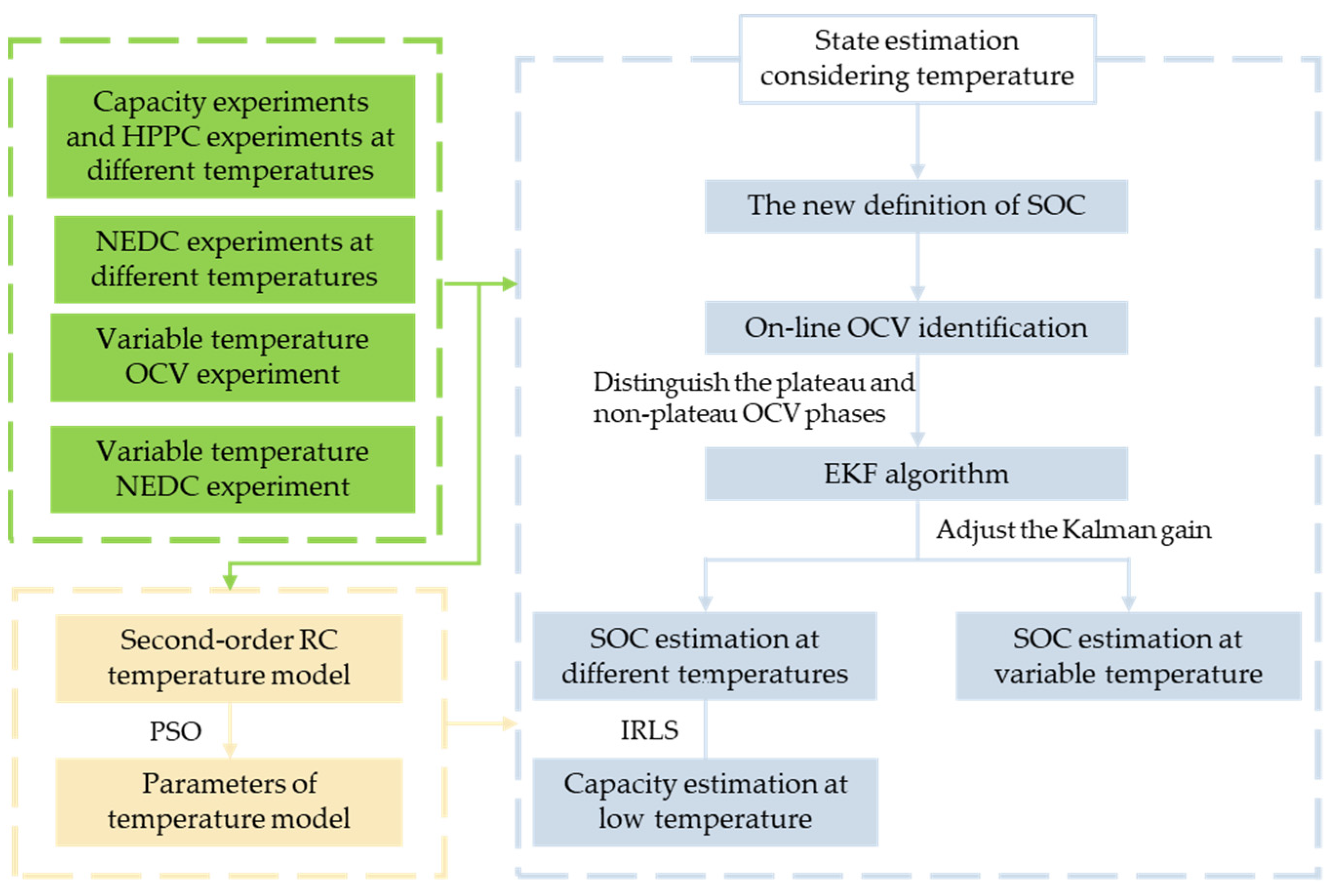
Thereby, in this paper, we propose a modified extended Kalman filter (EKF) algorithm. The LiFePO₄ battery is selected to verify the precision of SOC estimation results under various temperature scenarios and capacity estimation results under low temperature. Firstly, a second-order RC model considering temperature is established. Identifying all parameters of the model is performed by the PSO algorithm. Then, a new SOC definition is put forward according to temperature variation, which redefines the SOC cutoff point under different ambient temperatures. Furthermore, the OCVs at different temperatures are estimated based on the forgetting factor recursive least square (FFRLS) method, and the gain of EKF is adjusted between the plateau phase and non-plateau phase of the OCV curve. The SOC can subsequently be accurately estimated at different temperatures. In the meantime, through a discharging experiment under variable temperature conditions, the accuracy of the proposed method and the reliability of the battery model are verified. Finally, on the premise of the accurate SOC estimation of LiFePO₄ batteries at low temperatures, based on the principle of SOC electric quantity gain method, the iterative weighted least squares method is used to estimate the capacity of the battery at low temperatures.

2. Variable Temperature State Estimation Method

Estimation of the SOC is commonly carried out using the EKF algorithm, which is a method combining the ampere-hour integration method and terminal voltage calculation based on a battery model. The terminal voltage of the battery model is calculated based on OCV, and OCV is generally obtained through SOC–OCV curve interpolation or table query. However, there are two obvious plateau periods on the SOC–OCV curve of the LiFePO₄ battery. As a result, using the method of OCV table query, it is difficult to obtain an accurate OCV even with an accurate SOC. Inaccurate calculation of battery terminal voltage will lead to inaccurate estimation of the SOC in the next step. Therefore, how to use the EKF algorithm in the OCV plateau periods of LiFePO₄ batteries is a key problem. Moreover, setting a Kalman gain will largely determine the estimation accuracy of the EKF algorithm. An improved EKF algorithm is established in this section to estimate the SOC of a LiFePO₄ battery. The steps are as follows: Firstly, the OCV curve of a LiFePO₄ battery will be estimated online, and the noise of the EKF will be adjusted between zones according to the plateau and non-plateau phase of the estimated OCV curve. The advantages of combining the ampere-hour integration method and the battery model method of the EKF algorithm will be used to estimate SOC of the battery at different temperatures. Then, the SOC will be estimated at variable temperature dynamic conditions. Based on the SOC estimation results at low temperature, the weighted iterative least squares method will be utilized for estimating the battery capacity. The framework of this method is shown in Figure 1.

2.1. Battery Model and Parameter Identification

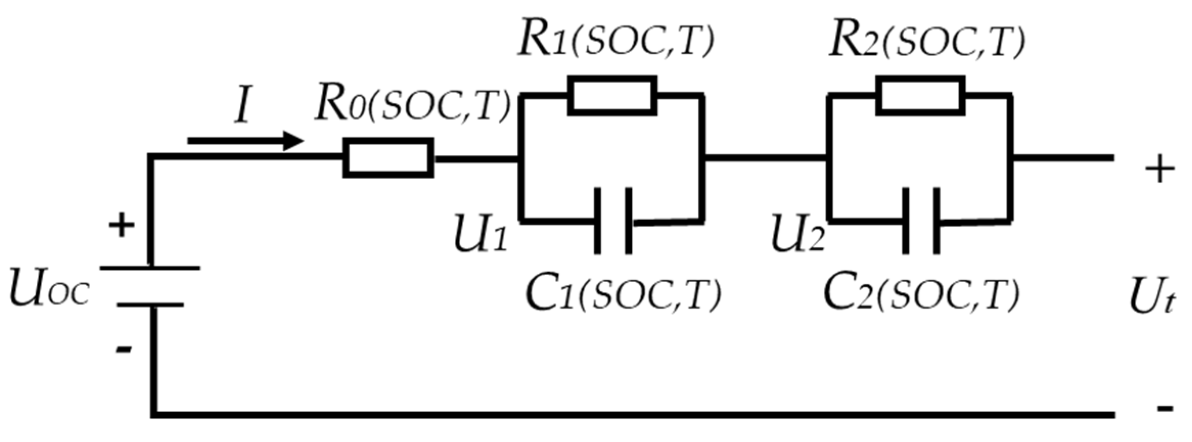
An accurate selection of the battery model is essential to achieve a high precision of the state estimation. Following a comprehensive consideration of the complexity, accuracy, implementation convenience and practical value of the chosen model, the RC equivalent circuit model is generally adopted. The higher the order of RC, the higher the accuracy. At the same time, since the variations in the parameters with temperature need to be considered, the second-order RC model considering temperature is an appropriate choice to simulate the characteristics of a LiFePO₄ battery. The structure of the selected model is illustrated in Figure 2.

In the aforementioned model, U_OC represents the OCV of the battery, I is the charging or discharging current, U_t is the terminal voltage and R₀ represents ohmic internal resistance. Polarization internal resistances, R₁ and R₂, are connected in parallel with polarization capacitors, C₁ and C₂, to form two RC structures. U₁ and U₂ are the voltages of the two RC structures, respectively, which are used to simulate the voltage rise and fall characteristics of the battery polarization. The measured current, I, and cell surface temperature, T, are the inputs of the established cell model. Meanwhile, U_t represents the output of the model. The state space equations and discretization equations obtained are as follows:

The equations of state spaces:

$$\frac{d(U_1)}{dt}=I(t)\frac{1}{C_1(SOC,T)}-\frac{1}{R_1(SOC,T)C_1(SOC,T)}{U}_1(t)$$

(1)

$$\frac{d(U_2)}{dt}=I(t)\frac{1}{C_2(SOC,T)}-\frac{1}{R_2(SOC,T)C_2(SOC,T)}{U}_2(t)$$

(2)

$$U(t)=U_{oc}(SOC,T)+I(t)\cdot R_0(SOC,T)+U_1(t)+U_2(t)$$

(3)

Equations (1)–(3) are simplified to obtain:

$$U_1(t)=U_1(t-1)e^{-\frac{\mathsf{\Delta }t}{{\tau }_1}}+I(t)R_1(1-e^{-\frac{\mathsf{\Delta }t}{{\tau }_1}})$$

(4)

$$U_2(t)=U_2(t-1)e^{-\frac{\mathsf{\Delta }t}{{\tau }_2}}+I(t)R_2(1-e^{-\frac{\mathsf{\Delta }t}{{\tau }_2}})$$

(5)

$$U(t)=U_{oc}(t)+I(t)R_0+U_1(t)+U_2(t)$$

(6)

where ${\tau }_1=R_1{C}_1$, ${\tau }_2=R_2{C}_2$, ${\tau }_1$ and ${\tau }_2$ are time constants and $\Delta t$ is the sampling interval.

Since the parameters in the model cannot be measured directly, experimental data will be utilized to identify these unknown parameters. In this paper, the PSO algorithm is selected for parameter identification for its fast calculation speed and low use of resources. The model parameters to be identified are as follows:

$$\theta =[R_{Cha},R_{Dch},R_1,{\tau }_1,R_2,{\tau }_2]$$

(7)

where $R_{Cha}$ indicates charging ohmic internal resistance and $R_{Dch}$ indicates discharging ohmic internal resistance. To evaluate the precision of the battery model, we take advantage of the rooted mean squared error (RMSE) between the terminal voltage of the model and the measured terminal voltage in the battery experiment. Therefore, the adaptability function of PSO is:

$$\widehat{F}({\widehat{\theta }}_k)=\sqrt{\frac{1}{N}{{\displaystyle \sum _{k=1}^N(U_k-{\widehat{U}}_k({\widehat{\theta }}_k))}}^2}$$

(8)

where $\widehat{F}({\widehat{\theta }}_k)$ indicates the RMSE at time k, N is the number of data points and $U_k$ and ${\widehat{U}}_k$ indicate the measured terminal voltage at time k and the terminal voltage estimated by the model at time k, respectively. ${\widehat{\theta }}_k$ is an estimate of the individual parameters in the model.

2.2. Improved EKF Algorithm

There are two goals that can be achieved with the improved EKF algorithm. On the one hand, the OCV curve of the battery can be determined online from the real-time data accurately. On the other hand, to improve the convergence speed of the algorithm and the ability to change parameters during identification, the forgetting factor, λ, is added to amplify the weight influence of the next iteration. In this way, it can increase the influence of new data in the dynamic system on the identification results. With respect to the established model incorporating the temperature factor, the FFRLS algorithm is employed for the OCV which is identified online for the LiFePO₄ battery. The form of recursive least squares method based on the standard is $y_k={\varphi }_k{\theta }_k+e_k$, and the specific process of FFRLS algorithm is shown in Figure 3.

λ is the forgetting factor, affecting the final estimation result with different values. If λ is too small, the increase in the weight of the old data will lead to a fluctuation or divergence of the identification result. If λ is too large and the weight of the old data is too small, the identification result will not track the dynamic parameters with time, and the convergence speed will slow down. In general, λ is set in the range of 0.95 to 1. After parameter modification, when λ = 0.98, the method can take both stability and convergence speed into account.

When the online estimation of is OCV finished, the plateau phase and non-plateau phase can be distinguished, and then the Kalman gain can be adjusted in the EKF algorithm. For dynamic nonlinear systems, when system noise and measurement noise are considered, Equations (9) and (10) are generally used to express the state space model of the system:

x_{k + 1} = f(x_k,u_k) + w_k

(9)

$$y_k=g(x_k,u_k)+v_k$$

(10)

According to the above state space model, taking $x_k={[SOC,U_1,U_2]}^T$ as the state variable, the charging and discharging current as the input and the estimated terminal voltage as the output, we obtain the discrete state space expressions:

$$x_{k+1}=A\cdot x_k+B\cdot I_k+w_k$$

(11)

$$U_{t,k}=U_{ocv}-U_{1,k}-U_{2,k}-I_k{R}_0+v_k$$

(12)

The initialization and iterative estimation equations of the EKF algorithm are shown in

Table 1. Iteration equations of the EKF algorithm.

Definition: ${\widehat{A}}_k=\frac{\partial f(x_k,u_k)}{\partial x_k}=\left[\begin{array}{ccc}1& 0& 0\\ 0& exp(-\mathsf{\Delta }t/{\tau }_1)& 0\\ 0& 0& exp(-\mathsf{\Delta }t/{\tau }_2)\end{array}\right]$ ${\widehat{C}}_k=\frac{\partial g(x_k,u_k)}{\partial x_k}=\left[\begin{array}{ccc}\frac{dOC{V}_k^{}(SO{C}_k^{})}{dSO{C}_k^{}}& -1& -1\end{array}\right]$ Here are the steps: Initialization: K = 0, initial state vector $x_0^{+}=E[x_0]$, initial bias $P_0^{+}=E[(x-{\widehat{x}}_0^{+}){(x-{\widehat{x}}_0^{+})}^T]$ Iterative calculation: When K = 1,2… Status vector time update: ${\widehat{x}}_k^{-}=f({\widehat{x}}_{k-1}^{+},u_{k-1})$ Error covariance matrix time update: ${\displaystyle {\sum }_{\tilde{x},k}^{-}={\widehat{A}}_{k-1}}{\displaystyle {\sum }_{\tilde{x},k-1}^{+}{\widehat{A}}^T{}_{k-1}}+{\displaystyle {\sum }_w}$ To calculate the Kalman gain: $L_k={{\displaystyle {\sum }_{\tilde{x},k}^{-}{\widehat{C}}_k^T[{\widehat{C}}_k{\displaystyle {\sum }_{\tilde{x},k}^{-}{\widehat{C}}_k^T+}{\displaystyle {\sum }_v}]}}^{-1}$ Status vector measurement update: ${\widehat{x}}_k^{+}={\widehat{x}}_k^{-}+L_k[y_k-g({\widehat{x}}_k^{-},u_k)]$ Error covariance matrix measurement updated: ${\displaystyle {\sum }_{\tilde{x},k}^{+}=(I-L_k{\widehat{C}}_k)}{\displaystyle {\sum }_{\tilde{x},k}^{-}}$

where ${\widehat{A}}_k$ and ${\widehat{C}}_k$ are the coefficient matrixes, $L_k$ is the Kalman gain, ${\displaystyle {\sum }_w}$ and ${\displaystyle {\sum }_v}$ are the covariance matrixes of the input measurement noise named $w_k$ and the output measurement noise named $v_k$, respectively. The covariance matrix, ${\displaystyle {\sum }_{\tilde{x},k}^{}}$, indicates the non-determinacy of the state estimation.

.

The OCV plateau of the LiFePO₄ battery is also known as the non-battery model reliability interval. Within this interval, an appropriate Kalman gain should be selected so that the EKF algorithm is even more inclined to trust the actual terminal voltage value measured by the voltage sensor. In this case, it is preferable to calculate the SOC using the method of ampere-hour integration. In the non-plateau phase of the battery, that is, the reliability interval of the battery model, it is more preferable to select the Kalman gain to obtain the terminal voltage from the EKF algorithm. In this case, the OCV table query method is preferred to estimate the SOC of the battery. Thereby, the key to solving the problem is to find the specific voltage value that distinguishes the OCV plateau period from the OCV non-plateau period.

2.3. Capacity Estimation Method

The discharging capacity of a battery will greatly reduce at low temperatures, which causes a tremendous impact on the pinpoint capacity estimation results at low temperature. At present, the SOC electric quantity gain method is commonly used to estimate the battery capacity. The variation in battery capacity is generally calculated by the ampere-hour integration method. After obtaining the SOC at different temperatures as described above, the capacity estimation at low temperature can be carried out based on the idea of the SOC charge gain method by using the result of the low temperature SOC estimation. The least square method is a common online estimation method of battery capacity by iterative calculations. Considering that the SOC estimation process will be affected by uncontrollable noise at low temperatures, the battery capacity is estimated using the weighted iterative least squares method.

The two-point method is a basis for the SOC electric quantity gain method. When the ∆Q of two points and the corresponding ∆SOC is calculated the battery capacity can be calculated from the ratio between the two points. The calculation formula is shown in Equation (13):

$$C_{norm}=\frac{\mathsf{\Delta }Q}{\mathsf{\Delta }SOC}=\frac{{\displaystyle {\int }_{t_1}^{t_2}\frac{\eta I(t)}{3600}dt}}{SOC(t_2)-SOC(t_1)}$$

(13)

where $SOC(t_1)$ and $SOC(t_2)$ represent SOC at the moments t₁ and t₂, respectively. I(t) is the charging and discharging current at time t and η is the coulomb efficiency, usually taken as 1.

The capacity estimation model for ordinary least squares (OLS) is:

$$y_i={\beta }_1+{\beta }_2{x}_i+v_i$$

(14)

where ${\beta }_1$ is a constant value, ${\beta }_2$ is a coefficient value (both are to be calculated) and $v_i$ is the noise.

Converting Equation (14) to the vector Formula (15) gives:

$$\left[\begin{array}{c}{y}_1\\ y_2\\ ⋮\\ y_n\end{array}\right]=\left[\begin{array}{cc}1& x_{11}\\ 1& x_{21}\\ ⋮& ⋮\\ 1& x_{n1}\end{array}\right]\left[\begin{array}{c}{\beta }_1\\ {\beta }_2\end{array}\right]+\left[\begin{array}{c}{v}_1\\ v_2\\ ⋮\\ v_n\end{array}\right]$$

(15)

Thereby, the battery capacity in the model can be calculated by Formula (16):

$$C_{norm}=1/{\beta }_2$$

(16)

The matrix form of Formula (15) is:

$$Y=X\cdot H+V$$

(17)

where Y is the observation vector corresponding to n*1, X represents the matrix of n*2, H is the parameter vector, $H={[{\beta }_1,{\beta }_2]}^T$ and V is the error vector of n*1. The capacity can be calculated using iteratively reweighted least squares (IRLS) using the OLS capacity estimation model.

$$S_E={\displaystyle \sum _{i=1}^n{(Y_i-{\beta }_1-{\beta }_2{x}_i)}^2={\displaystyle \sum _{i=1}^n{v}_i^2}}$$

(18)

where $v_i$ represents the residuals. If the influence function, ρ, is chosen as the sum of the squares of the residuals, the objective function is transformed to:

$$S_E={\displaystyle \sum _{i=1}^n\rho (Y_i-{\beta }_1-{\beta }_2{x}_i)={\displaystyle \sum _{i=1}^n\rho (v_i)}}$$

(19)

$S_E$ deflects from $\beta$ so that it is 0, obtaining the equation:

$${\displaystyle \sum _{i=1}^n\phi (Y_i-{\beta }_1-{\beta }_2{x}_i)x_i=0}$$

(20)

where $\phi (x)$ is the derivative of $\rho (x)$.

Introducing $S=\frac{med(\left|v_i\right|)}{0.6745}$ in the weight function yields the standardized residuals $u_i=\frac{v_i}{S}=\frac{0.6745\cdot v_i}{med(\left|e_i\right|)}$, where med represents the absolute median of the dispersion calculation.

Formula (20) can then be written as:

$${\displaystyle \sum _{i=1}^n\phi (Y_i-{\beta }_1-{\beta }_2{x}_i)x_i=}{\displaystyle \sum _{i=1}^n\phi (u_i)x_i=}{\displaystyle \sum _{i=1}^n\frac{\phi (u_i)}{u_i}}\cdot u_i\cdot x_i={\displaystyle \sum _{i=1}^n{w}_i}\cdot u_i\cdot x_i=0$$

(21)

where $w_i=\frac{\phi (u_i)}{u_i}$ is the sample weight of the observation of number i. Formula (18) is vectorized and brought into the matrix to obtain:

$$X^{T}WY=X^{T}WXH$$

(22)

Obtaining the parameter estimates as:

$${\widehat{H}}_w={(X^{T}WX)}^{-1}{X}^{T}Y$$

(23)

Once the parametric vector ${\widehat{H}}_w={[{\beta }_1,{\beta }_2]}^T$ is obtained, the capacity estimate can be calculated by Formula (16).

3. Experiments

3.1. Basic Performance Test at Different Temperatures

In this paper, a LiFePO₄ battery from Tianjin Lishen Battery Company was selected to carry out the basic performance experiments at different temperatures. The battery was placed in a temperature chamber which could achieve a high temperature and low temperature conversion during the experiment. In addition, the Xinwei battery test system was used to conduct temperature variation experiments at different temperatures and different rest times. A brief description of the basic parameters of the battery is provided in

Table 2. Basic performance parameters of experimental battery.

Parameters	Numeric Value
Nominal capacity (Ah)	20
Nominal voltage (V)	3.2
Charging cutoff voltage (V)	3.65 ± 0.5
Discharging cutoff voltage (V)	2.0
Standard charging and discharging current (A)	1/3C
Charging temperature (°C)	0~45
Discharging temperature (°C)	−20~60

.

The standard capacity of the LiFePO₄ battery was tested at 45 °C, 25 °C, 5 °C and −15 °C. In an effort to obtain the standard charging and discharging capacities at different ambient temperatures, a current of 6.67 A, which is 1/3C, was used to charge and discharge the battery. In addition, the hybrid pulse power characteristic (HPPC) test was proposed to obtain the internal resistance at each temperature. Meanwhile, the dynamic working condition experiments were conducted at four temperatures to provide data for the estimation of SOC.

3.2. Variable Temperature OCV Experiment

An important tool which can reflect the operating characteristics is the OCV–SOC relationship curve of one battery. The OCVs of the same battery will be different when the temperature changes, and there is an OCV plateau in the OCV of a LiFePO₄ battery. Therefore, analyzing the OCV performance of the LiFePO₄ battery at different temperatures was crucial. An original experiment method was proposed to attain the OCV of the full range of the SOC. Firstly, the battery temperature was initially set at 25 °C and fully charged in this scenario, followed by 45 °C, 25 °C, 5 °C and −15 °C settings for the temperature chamber. The corresponding rest time was set to 3 h, 3 h, 4 h and 5 h, respectively, so as to obtain the OCV of the SOC node at each temperature. After the rest time, the temperature chamber was adjusted to the temperature of 25 °C, and the next SOC point can be obtained by constant discharging current. The above steps are repeated to obtain the OCVs in the full SOC range at different temperatures. Figure 4 shows the flow chart of the OCV experiment at variable temperatures.

3.3. Experiment to Determine the Upper and Lower Limits of SOC at Different Temperatures

The SOC reflects the discharging capacity of a battery, which is defined as the proportion of the remaining discharging capacity to the total capacity. As temperatures and aging effect the overall discharging capacity of a lithium-ion battery, the SOC used to reflect the residual discharging capacity of the battery must also take into account these factors. SOC values for batteries are inconsistent at different temperatures when the standard capacity test method is used to charge and discharge the battery to the cutoff voltage. Thus, it is necessary to redefine the SOC and define the upper and lower limits of the SOC when the ambient temperature is different. In this paper, the SOC at 25 °C was used as the benchmark, meaning the range of SOC at 25 °C was 0 to 100%, and the upper and lower limits of SOC at other temperatures changes as the temperature changes.

To determine the two limits of SOC at different temperatures, the following experiments were conducted:

(1) At 25 °C, the battery was charged with 1/3C constant current to charge it to the charging cutoff voltage, and then it was charged to the charging cutoff current with constant voltage. At this point, the battery SOC was 100%. Then, it was adjusted to rest for a certain time at different temperatures, and then discharged to the lower limit of voltage at 1/3C. In this process, this ratio was the lower limit of SOC at this temperature, which is the remaining battery capacity divided by the total discharge capacity at 25 °C, as shown in Equation (24).

$$SO{C}_L^T=\frac{Ca{p}_{discha}^{25}-Ca{p}_{discha}^T}{Ca{p}_{discha}^{25}}$$

(24)

where $SO{C}_L^T$ denotes the lower limit of the SOC when the redefined temperature is T, $Ca{p}_{discha}^{25}$ represents the discharging capacity at 25 °C, $Ca{p}_{discha}^T$ is the actual discharging capacity at temperature T and T is the ambient temperature in °C.

(2) At 25 °C, the battery was charged with 1/3C current to the lower limit of voltage for discharging, at which time the battery SOC was 0%. Then, the battery was maintained at other temperatures for a certain time, and then a constant current was applied to charge the battery to the upper voltage limit. In this process, the ratio was the upper limit of SOC at this temperature, which is the capacity at this temperature, to the battery capacity at 25 °C, as indicated in Equation (25).

$$SO{C}_U^T=\frac{Ca{p}_{cha}^T}{Ca{p}_{cha}^{25}}$$

(25)

where $SO{C}_U^T$ is the upper limit of SOC when the redefined temperature is T, $Ca{p}_{cha}^{25}$ is the charging capacity at 25 °C and $Ca{p}_{cha}^T$ is the actual charging capacity at temperature T.

3.4. Variable Temperature Dynamic Working Condition Experiment

Based on the previous dynamic working condition experiments at different temperatures, estimations of the SOC at different temperatures were calculated. However, the battery works in an environment with variations in temperature, and the accuracy of SOC estimation should be considered in terms of these environmental changes. Thus, this section adjusts the ambient temperature change for the experiment of continuous NEDC discharging condition of the battery. After being fully charged at 25 °C, the battery was put in the temperature chamber and the temperature was set to imitate the ambient temperature in an actual application. Meanwhile, the battery was discharged under continuous NEDC conditions to achieve the simultaneous current changes with ambient temperature.

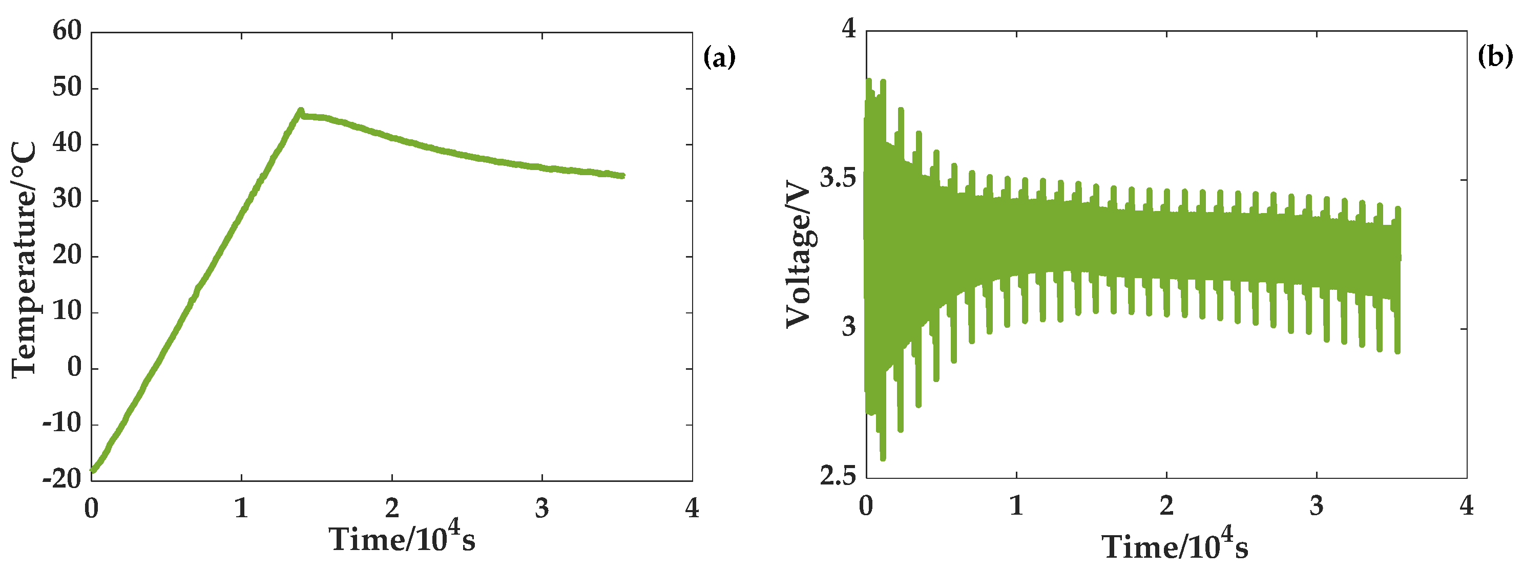
Two experiments of a temperature rise and a temperature drop were carried out to satisfy the temperature changes. The temperature and voltage curves for the rising temperature scenario are given in Figure 5. The ambient temperature where the battery is located gradually rises from −18 °C to 45 °C at a rate of 0.3 °C/min. At this time, the program of the temperature chamber stops, and the temperature gradually drops to 35 °C. When the battery reaches a low temperature, the terminal voltage is greatly affected by the temperature and changes sharply. At one point, the cutoff voltage of the battery reaches 3.8 V. With a gradual rise in temperature, the battery terminal voltage changes gradually stabilize. As shown in Figure 6, the temperature of the temperature chamber drops gradually from 45 °C to −12 °C at a rate of 0.3 °C/min. At this time, the program of the temperature chamber stops, and the temperature gradually rises to 15 °C. Additionally, the terminal voltage curve shows that the terminal voltage changes sharply when the battery is at a low temperature. As the temperature rises gradually, the battery terminal voltage changes steadily.

4. Results

4.1. Experimental Results of Variable Temperature OCV

The variable temperature experiment was conducted at four temperatures, and all of them discharge at 25 °C to the next SOC point. Therefore, the SOC points at different temperatures are correspond well. In addition, the whole battery electric quantity can be released at 25 °C; thus, the OCV at all SOC points can be obtained. The OCV curves at the four temperatures show low fluctuation and are practically equal, as shown by the results of the variable temperature experiment. As a result, the model established in this study will not take into account the effect of temperature on OCV in order to reduce the complexity of the model and increase computational efficiency. The OCV–SOC curve at 25 °C will be adopted uniformly.

The battery SOC is stable when discharged at 25 °C, which is reflected in the OCV variation with SOC at different temperatures. Figure 7b reveals that the difference between the OCV at 25 °C and every other temperature is negligible. Thereby, the OCVs at different temperatures are considered to be same in the whole range of the SOC in this paper.

4.2. Parameter Identification Results

Figure 8 displays the parameters identified by the PSO algorithm using data from HPPC experiments conducted at different temperatures. The results demonstrate that changes in temperature and SOC have an impact on the charging and discharging ohmic internal resistance, two polarization internal resistances, and two time constants. In the following SOC estimation process, the model parameters are determined according to different SOC and different temperatures, which can meet the whole calculation requirements at different ambient temperatures and SOC conditions.

4.3. Fitting the SOC Upper and Lower Limit Functions

According to the actual charging and discharging electric quantity, calculations are performed using the aforementioned defined upper and lower limits of the SOC at each temperature. The final range of upper and lower limits of SOC at different temperatures are shown in Figure 9.

The upper and lower limits of the SOC function can be acquired by curve fitting in accordance with the determined upper and lower limits of SOC at four temperatures. Based on the results of the fitting, the two limits of the SOC at other temperatures, such as 0 °C, can be simulated. The fitting curves are shown in Figure 10.

SOC upper limit function:

$$SO{C}_U^T=0.2671\cdot e^{0.08937T}+97.51$$

(26)

SOC lower limit function:

$$SO{C}_L^T=9.899\cdot e^{-0.08702T}-1.115$$

(27)

Considering this figure, it is apparent that the fitting curves are capable of displaying the actual upper and lower limits of SOC with accuracy. Thus, SOC estimations and capacity estimations will be carried out based on this result.

4.4. Estimation Results of SOC at Different Temperatures and Variable Temperatures

The online OCV estimation of the LiFePO₄ battery under different ambient temperatures was carried out by the method of online OCV identification. Figure 11 displays the estimation result taking 45 °C as an example.

The error in the estimation results at the beginning and the end of OCV are relatively large. However, the purpose of online OCV estimation in this paper is to distinguish the plateau and non-plateau OCV phases of a LiFePO₄ battery. It is worth noting that there is a significant difference in the estimated OCV between the plateau and non-plateau phases. Consequently, during the low SOC interval, large OCV estimation errors will not have an effect on the accuracy of subsequent SOC estimation results. In Section 4.1, the OCV curves at different temperatures obtained by the variable temperature experiment were considered to be same, and so is the plateau phase and non-plateau phase of the OCV curves at different temperatures. Therefore, the OCV curve at 25 °C in the variable temperature experiment is applied uniformly. The OCV curve and the two plateau periods are shown in Figure 12. The red rectangles show the two OCV plateau periods (3.290 V to 3.298 V and 3.331 V to 3.334 V) of the LiFePO₄ battery range. The rest of OCV regions are non-plateau periods. Thereby, a specific value to distinguish the plateau phase from the non-plateau phase of the battery OCV can be obtained.

After distinguishing the plateau phase from the non-plateau phase based on the OCV estimation results, the NEDC experiment results at different temperatures, the OCV–SOC curve at a temperature of 25 °C and the discharging capacity will be used to estimate the SOC. This is for the sake of validating the fast convergence of the improved EKF algorithm tracking. On the other hand, considering that the capacity error will affect the SOC estimation, 10% of the original SOC error and 10% of the capacity error are introduced. The estimation results and errors at 45 °C, 25 °C, 5 °C and −15 °C are illustrated in Figure 13.

In the plateau phase, the algorithm tends to be calculated by the ampere-hour integration method. Due to the capacity error, there exists a cumulative error in the SOC calculation. In the non-plateau period, the algorithm tends to be calculated by the battery model combined with the improved EKF method. The accumulated error is corrected quickly and follows the real SOC. The above results demonstrate that the LiFePO₄ battery SOC can be accurately estimated at four ambient temperatures with the proposed method, and the maximum error is no more than 4%.

In the process of SOC estimation at variable temperatures, the battery model parameters for the full SOC range at that temperature are acquired first based on the ambient temperature. Then, the model parameter combination of the SOC is found according to the SOC estimated value at this time. This cycle is iterated to achieve the application of accurate model parameters at different ambient temperatures and SOC. For verifying the reliability of the algorithm, an error of 5% was set for both the SOC and capacity initial values. In addition, noise was added to the current and voltage in the input to simulate an actual sensor. These two variable temperature experiments produced results which are given in Figure 14 and Figure 15. The SOC errors fluctuate around 0%, and the estimated SOC of the two experiments with variable temperature can quickly converge to the real SOC. Under the condition that the temperature and current change simultaneously, the final accuracy of SOC estimation is within 3%.

In conclusion, with the conditions of SOC initial error, capacity error and current and voltage drift, using the improved EKF algorithm, the SOC estimation accuracy and robustness are maintained at variable temperatures.

4.5. Capacity Estimation

To confirm the accuracy of the IRLS algorithm for estimating the LiFePO₄ battery capacity at low temperatures, NEDC experiments were carried out on fresh and aged LiFePO₄ batteries at 0 °C. The battery SOC at 0 °C was first estimated with the improved EKF algorithm. Afterwards, the IRLS algorithm was used to estimate the capacity by iterative calculations. The results of the capacity estimation are presented in

Table 3. Basic performance parameters of the battery.

	Capacity Estimates	Capacity Experimental Values	Capacity Errors
Fresh battery	20.50 Ah	20.53 Ah	0.15%
Aged battery	19.56 Ah	19.43 Ah	0.67%

. Due to the precise SOC estimation result at 0 °C, the capacity error estimated by the IRLS algorithm at 0 °C is no more than 1%. As a result, battery capacity estimation by the IRLS algorithm in the whole range of SOC can maintain a high accuracy at low temperature. Meanwhile, the estimation error is stable for both fresh and aged batteries.

5. Conclusions

For the purpose of achieving an accurate estimation of the SOC of a LiFePO₄ battery at different and variable temperatures, an improved EKF algorithm is proposed. Firstly, with the forgetting factor, the OCV curve of the battery is identified online using the least square method. Then, the OCV values of the plateau phase and non-plateau phase are distinguished by the OCV curve at uniform temperature, and the Kalman gain is adjusted between the zones to accurately estimate the SOC of the full range. In addition, for estimating the variable temperature SOC, we drew upon a variable temperature NEDC experiment. The results show that all SOC errors are within 3%. On account of the pinpoint estimation of low temperature battery SOC, the low temperature battery capacity is estimated through the use of the IRLS algorithm. A high degree of accuracy is observed in the capacity estimation results for both fresh and aged batteries at low temperature, with errors all within 1%.