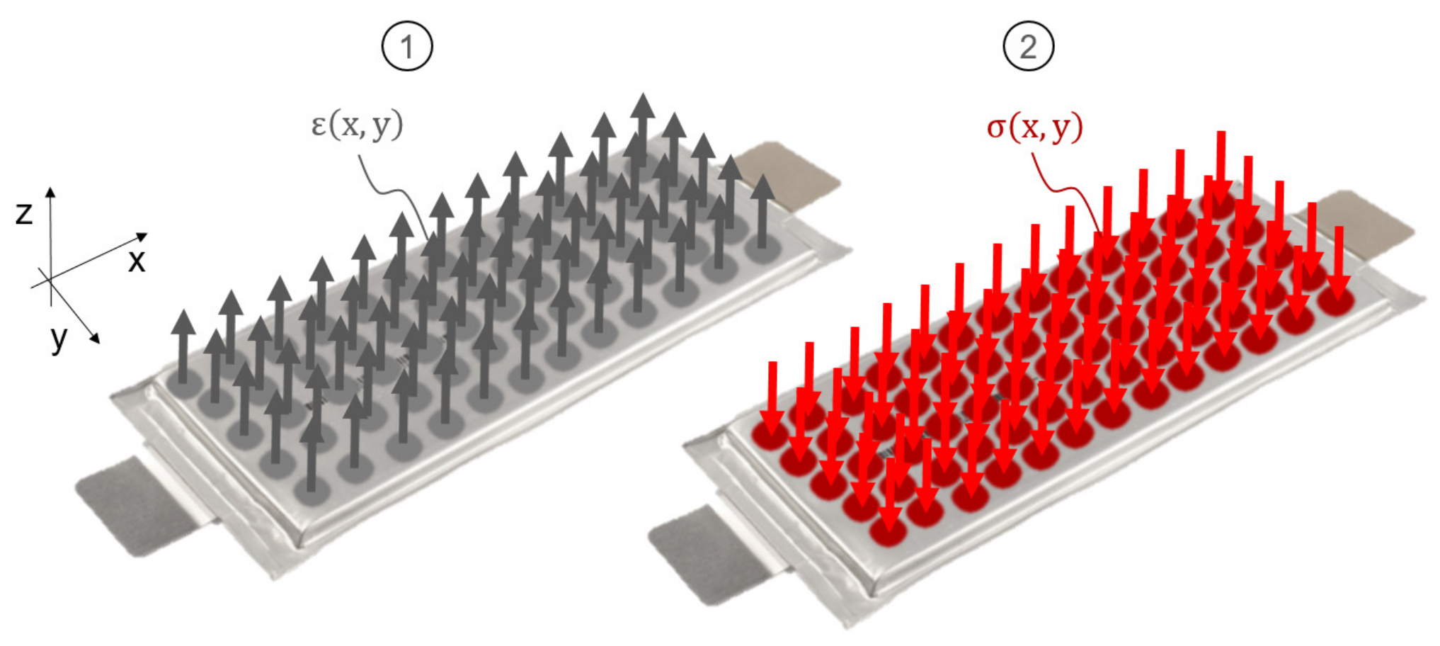
Figure 1.
The schematic representation of the homogeneous displacement and pressure field, which is assumed for the modelling in order to neglect the location dependence for the time being.
Figure 1.
The schematic representation of the homogeneous displacement and pressure field, which is assumed for the modelling in order to neglect the location dependence for the time being.
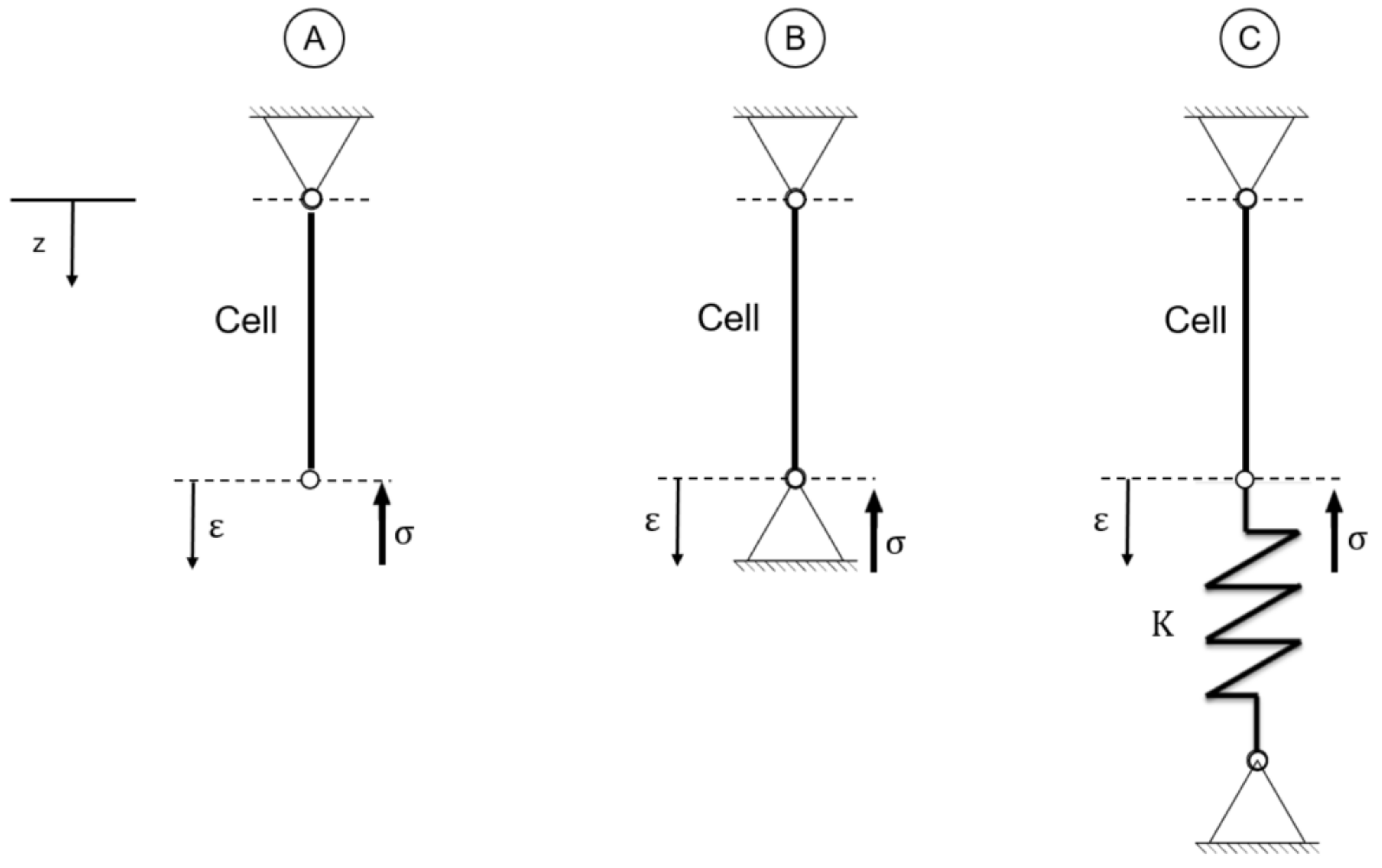
Figure 2.
Basic mechanical scenarios of a homogeneous cell swelling. Scenario (A) describes the constant force state; (B) describes the constant gap state; and (C) describes a constant stiffness state. All three scenarios are theoretically investigated using the model derived previously.
Figure 2.
Basic mechanical scenarios of a homogeneous cell swelling. Scenario (A) describes the constant force state; (B) describes the constant gap state; and (C) describes a constant stiffness state. All three scenarios are theoretically investigated using the model derived previously.
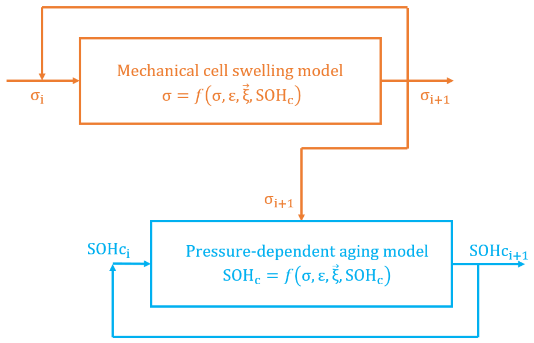
Figure 3.
Schematic representation of the model equations and the coupling. The upper loop represents the mechanical model, which is independent of the ageing model. The lower loop represents the ageing model, which depends on the mechanical model and is therefore coupled.
Figure 3.
Schematic representation of the model equations and the coupling. The upper loop represents the mechanical model, which is independent of the ageing model. The lower loop represents the ageing model, which depends on the mechanical model and is therefore coupled.
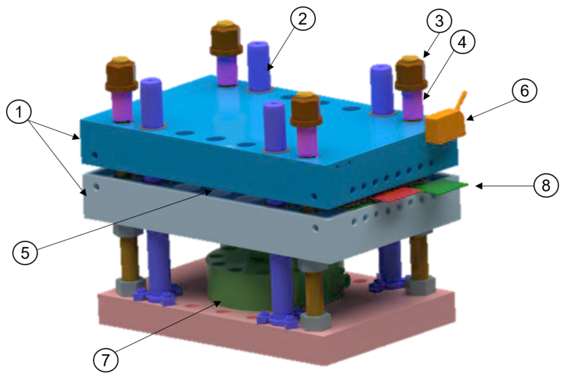
Figure 4.
Representation of the jig setup. The cell (5) is inserted into two large aluminium plates (1) which are supported by compression springs (4), threaded rods (3) and guide columns (2). The force is measured by a force box (7), which is mounted under the intermediate plate and measures a force via the vertical displacement of the plates. The design criteria for the plates are to minimise deformation and to ensure a homogeneous pressure distribution across the cell. The thickness is increased by measuring the distance between the plates. This is done using a laser sensor (6). To measure the distance from the outside, an insert plate (8) is placed under the cell.
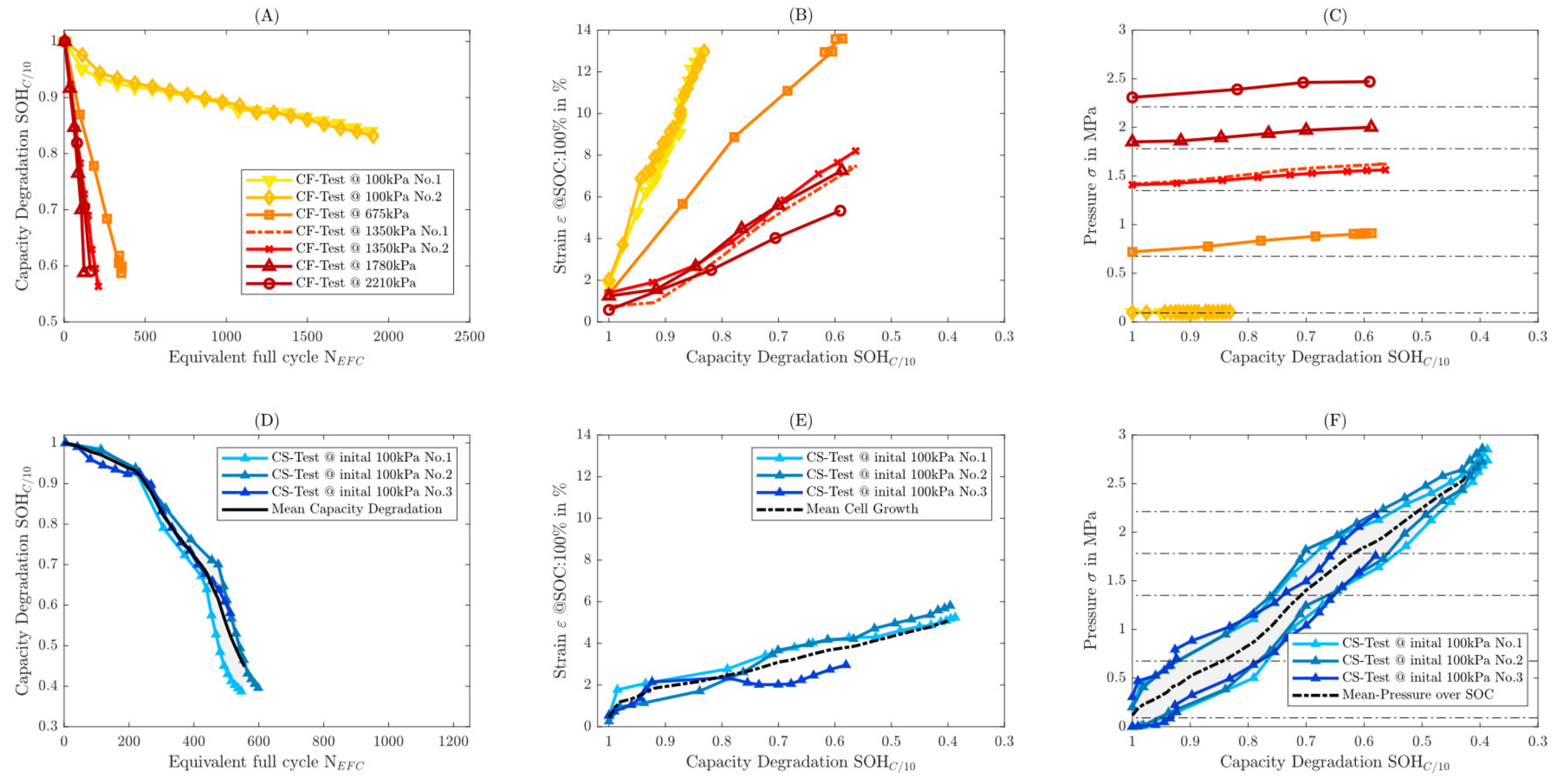
Figure 5.
Overview of the result variables on constant force measurements (A–C) and constant stiffness measurements (D–F). (A,D) shows the capacity degradation, (B,E) show the cell growth (at = 100%) over the . In (C,F) is the Pressure evolution over the shown.
Figure 5.
Overview of the result variables on constant force measurements (A–C) and constant stiffness measurements (D–F). (A,D) shows the capacity degradation, (B,E) show the cell growth (at = 100%) over the . In (C,F) is the Pressure evolution over the shown.
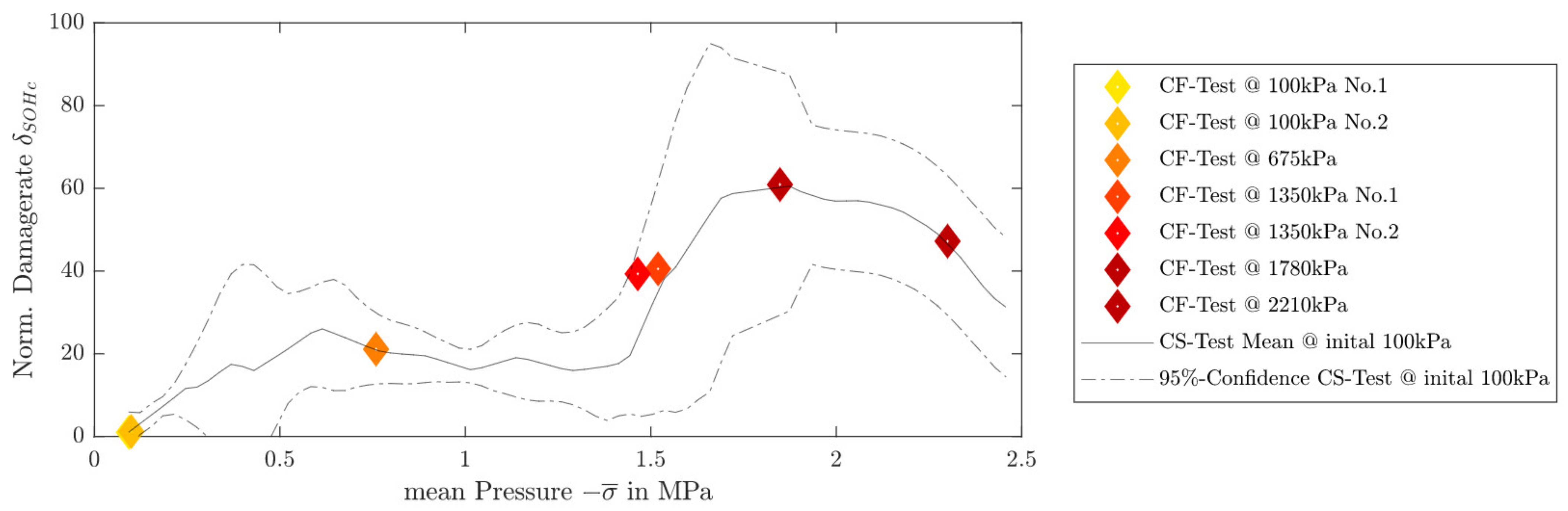
Figure 6.
The normalized damage rate pressure diagram shows the pressure influence on capacity aging. The diagram shows the damage rates resulting from the constant force measurement via the red diamonds and the damage rate progression from the CS measurement as a continuous measurement.
Figure 6.
The normalized damage rate pressure diagram shows the pressure influence on capacity aging. The diagram shows the damage rates resulting from the constant force measurement via the red diamonds and the damage rate progression from the CS measurement as a continuous measurement.
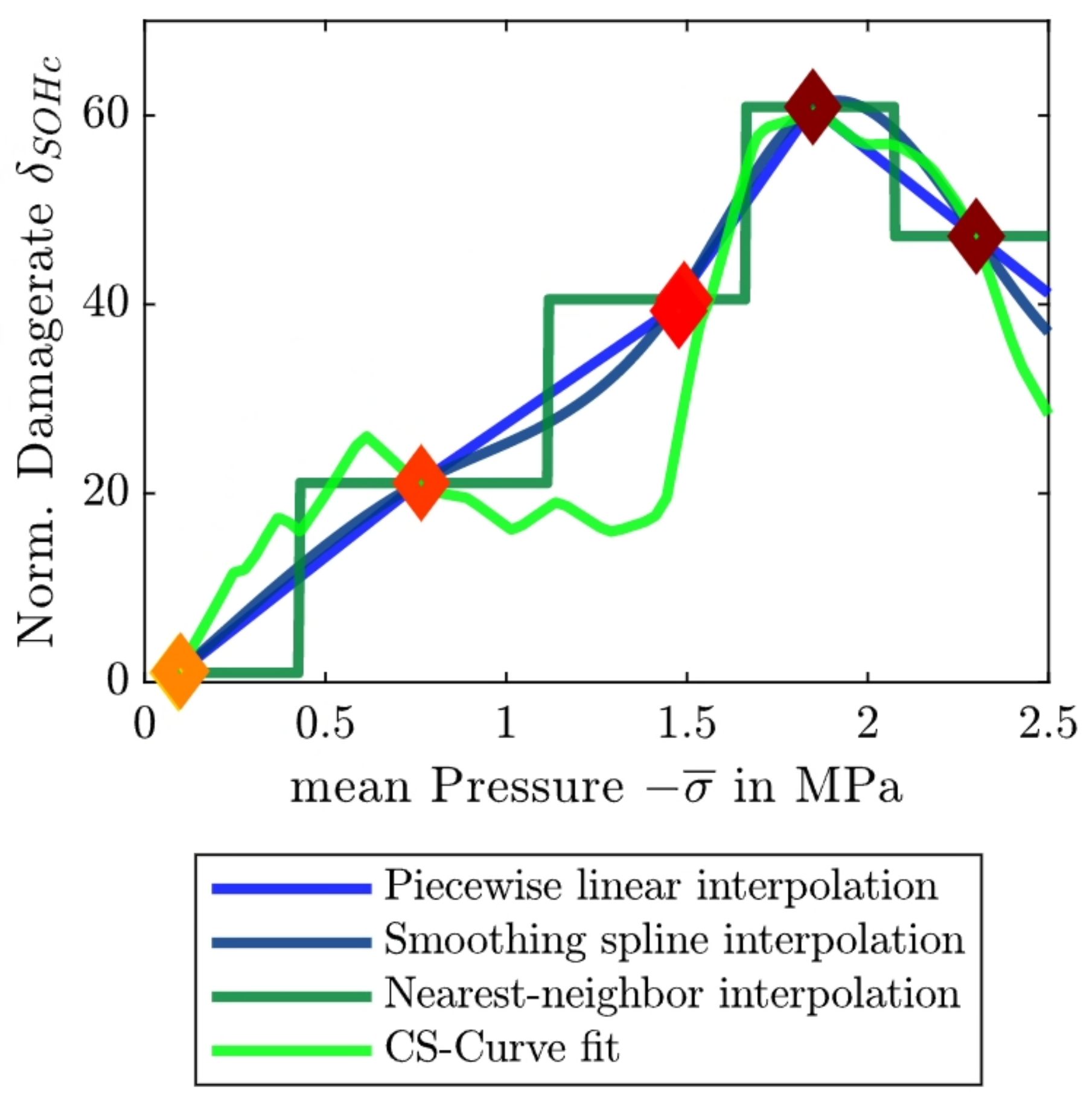
Figure 7.
Comparison of the four different interpolation methods that are investigated in the study. The diamonds correspond to the damage rates based on the CF tests.
Figure 7.
Comparison of the four different interpolation methods that are investigated in the study. The diamonds correspond to the damage rates based on the CF tests.
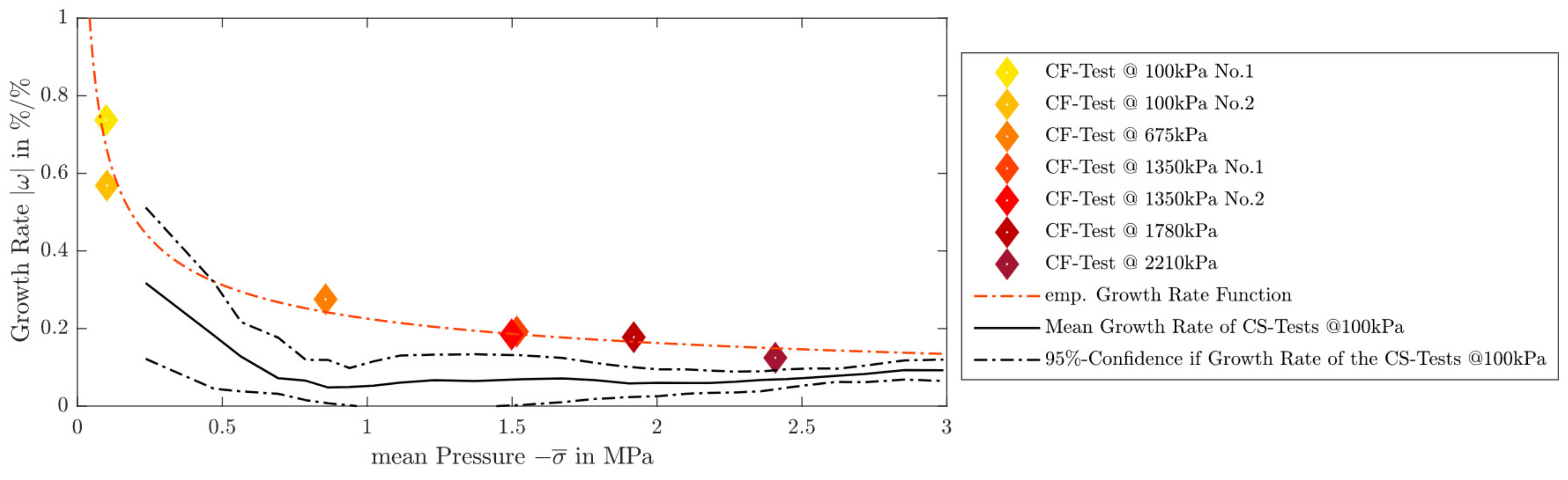
Figure 8.
The normalized growth rate pressure diagram shows the growth behavior, related to the aging of the cell as a function of the applied pressure normalized growth rate pressure diagram. The diagram contains the growth rates resulting from the constant force measurement via the red diamonds and the damage rate progression from the CS measurement as a continuous measurement.
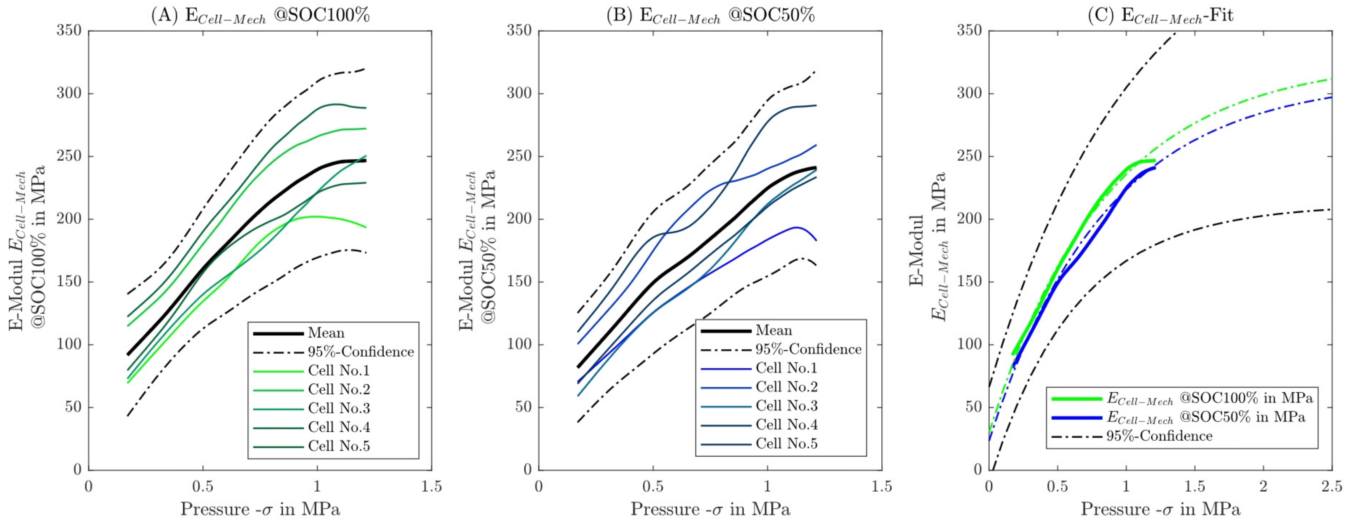
Figure 9.
Representation of elastomechanical E−Modu via pressure. In (A), the measurements are shown at a SOC of 100% and in (B) at a SOC of 50%. In addition, the mean value and 95% confidence range were evaluated. In (C) the empirical regression for the mean courses at SOC 100% and 50% and with the 95% confidence interval is shown.
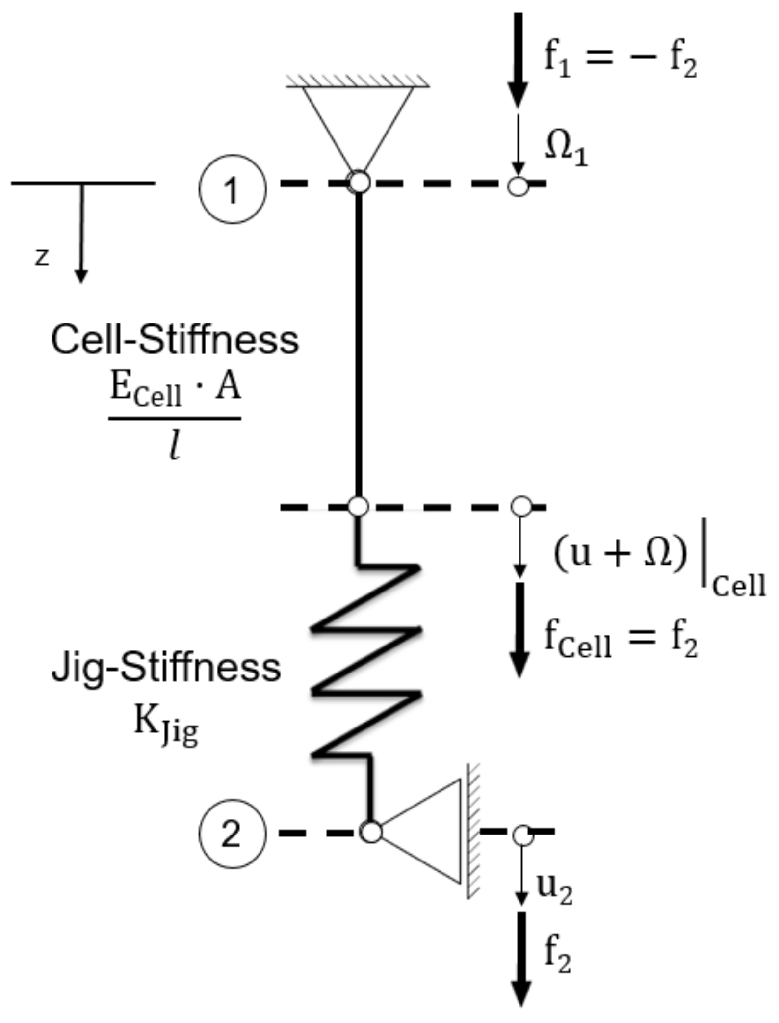
Figure 10.
Mechanical equivalent circuit diagram for clamping conditions of the cell in the structure.
Figure 10.
Mechanical equivalent circuit diagram for clamping conditions of the cell in the structure.
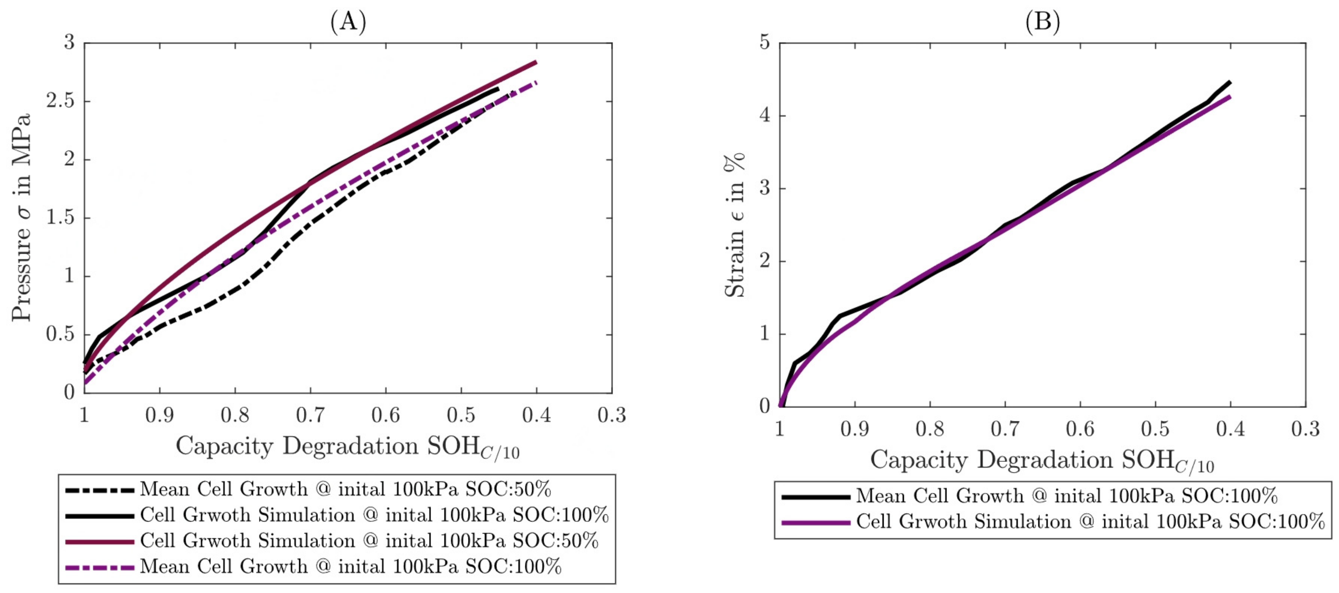
Figure 11.
Comparison of mechanical simulation with measurement. In (A), the measured pressure development over aging is compared with the simulation at a SOC = 100 and 50%. In (B) is the measured irreversible growth compared to the simulation.
Figure 11.
Comparison of mechanical simulation with measurement. In (A), the measured pressure development over aging is compared with the simulation at a SOC = 100 and 50%. In (B) is the measured irreversible growth compared to the simulation.
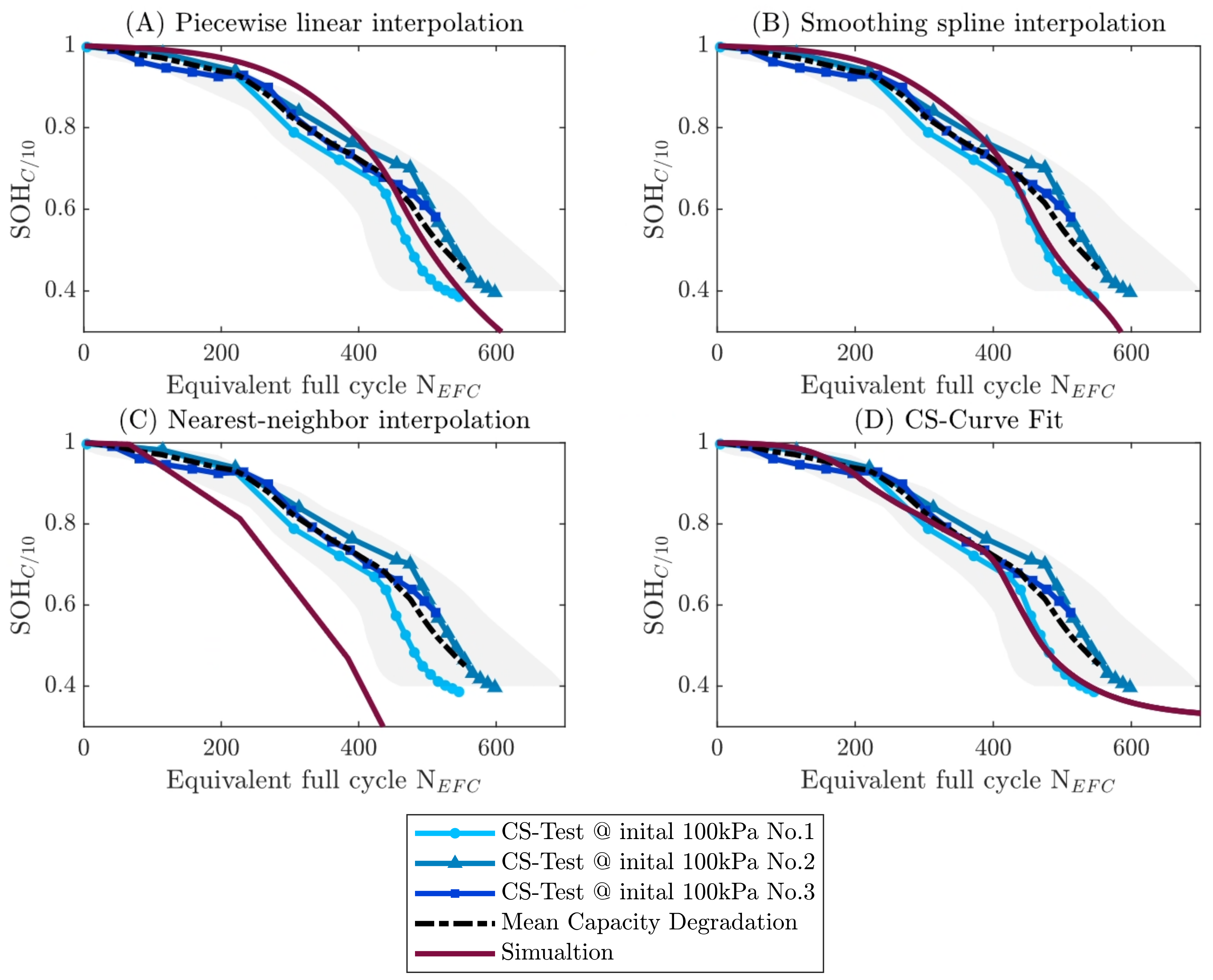
Figure 12.
Complete comparison measurements with the aging simulation. The subplots are divided according to the four interpolation methods used for the simulation. In the plots, the individual measurements are shown in blue, the mean is shown in black dashed lines, the 95% confidence interval of the measurements is shown in grey as a grey corridor, and the ageing simulation is shown in purple. The two interpolation methods (A,B) lead to very comparable results, whereas methods (C,D) are very different: (C) shows the largest deviation, which occurs first and then remains. In (D) the smallest deviation can be seen, as here only the deviation from the mechanical forecast has an effect.
Figure 13.
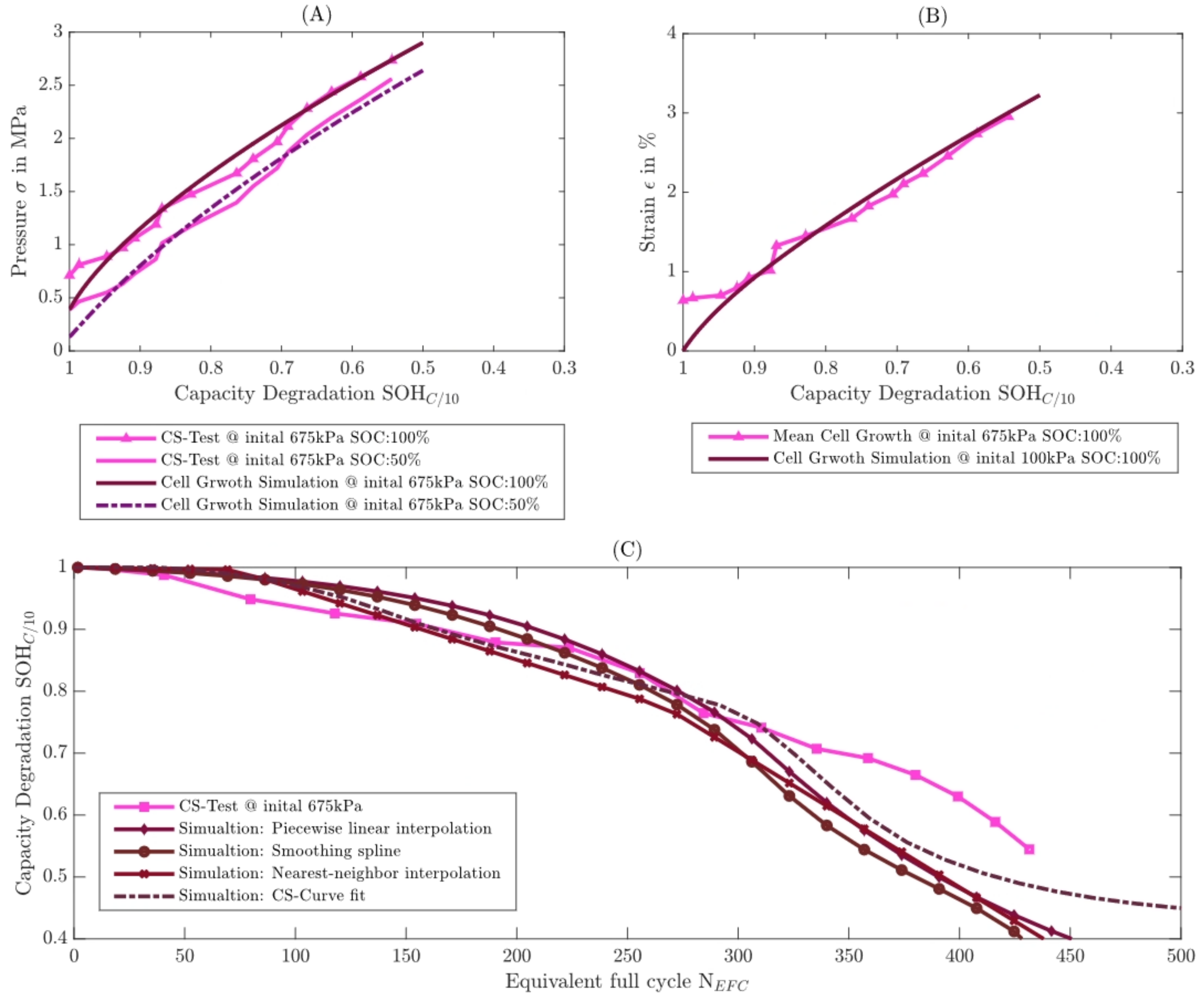
Complete simulation and measurement comparison with validation measurements II. In (A), the measured pressure development over aging is compared with the simulation at a SOC = 10 and 50%. In (B) is the measured irreversible growth compared to the simulation. In (C) the comparison between the measured capacitance aging with four different simulations is shown.
Figure 13.
Complete simulation and measurement comparison with validation measurements II. In (A), the measured pressure development over aging is compared with the simulation at a SOC = 10 and 50%. In (B) is the measured irreversible growth compared to the simulation. In (C) the comparison between the measured capacitance aging with four different simulations is shown.
Table 1.
Single-factor constant force testplan.
Table 1.
Single-factor constant force testplan.
| Preload Condition @SOC30% | Charge-Profile | Discharge-Profile | Temperature | DOD | n |
|---|
| 100 kPa | 1.3 C | 1.3 C | 35 °C | 100% | 2 |
| 675 kPa | 1.3 C | 1.3 C | 35 °C | 100% | 1 |
| 1350 kPa | 1.3 C | 1.3 C | 35 °C | 100% | 1 |
| 1780 kPa | 1.3 C | 1.3 C | 35 °C | 100% | 1 |
| 2210 kPa | 1.3 C | 1.3 C | 35 °C | 100% | 1 |
Table 2.
Validation measurement Constant stiffness testplan.
Table 2.
Validation measurement Constant stiffness testplan.
| Preload Condition @SOC30% | Charge-Profile | Discharge-Profile | Temperature | DOD | n |
|---|
| 100 kPa | 1.3 C | 1.3 C | 35 °C | 100% | 3 |
Table 3.
Empirical description of elasto-mechanical cell stiffness.
Table 3.
Empirical description of elasto-mechanical cell stiffness.
| Parameter | SOC = 50% | SOC = 100% | Unit |
|---|
| α | 288.5 | 297.1 | MPa |
| 0.8403 | 0.8474 | MPa |
| γ | 23.86 | 30.22 | MPa |
Table 4.
Test matrix for validation measurement.
Table 4.
Test matrix for validation measurement.
| Measurement Series | Preload Condition @SOC30% | Charge-Profile | Discharge-Profile | Temperature | DOD | n |
|---|
| I | 100 kPa | 1.3 C | 1.3 C | 35 °C | 100% | 3 |
| II | 675 kPa | 1.3 C | 1.3 C | 35 °C | 100% | 1 |
Table 5.
Overview of mean square deviations.
Table 5.
Overview of mean square deviations.
| Interpolation Method | | σstd | 95%-CL | 99%-CL |
|---|
| Piecewise linear interpolation | 18.55 | 13.52 | 26.5 | 34.83 |
| Smoothing spline interpolation | 16.62 |
| Nearst-neighbor interpolation | 53.83 |
| CS-Curve fit | 10.57 |


