Abstract
Accurate State-of-Charge estimation is crucial for applications that utilise lithium-ion batteries. In real-time scenarios, battery models tend to present significant uncertainty, making it desirable to jointly estimate both the State of Charge and relevant unknown model parameters. However, parameter estimation typically necessitates that the battery input signals induce a persistence of excitation property, a need which is often not met in practical operations. This document introduces a joint state of charge/parameter estimator that relaxes this stringent requirement. This estimator is based on the Generalized Parameter Estimation-Based Observer framework. To the best of the authors’ knowledge, this is the first time it has been applied in the context of lithium-ion batteries. Its advantages are demonstrated through simulations.
1. Introduction
In the current energetic scenario, decarbonisation of the electrical grid is a primary objective. In this context, energy storage plays a crucial role, as the use of Electric Vehicle (EV) is spreading [1,2] and the penetration of renewable energy sources in the grids increases [3]. While there are several Energy Storage System (ESS), lithium-ion batteries (LIBs) are currently the most popular technology, as they are flexible, efficient and offer a good trade-off between energy density and power density [4,5].
In real applications, Li-ion batteries need to be monitored to ensure that their operation is within safety limits. Battery Monitoring System (BMS) ensure this objective by monitoring and managing several variables of the cell [6]. Among all these variables, the most important one is the State of Charge (SoC), which can be defined as the relation between the remaining capacity of the battery compared to the nominal capacity. The knowledge of SoC allows system monitoring to occur while providing the users with information about how much energy is stored in the battery, facilitating the decision-making process. Simple examples of this can be the range of an EV or the charging/discharging management of a battery connected to a microgrid. A more concrete example is the charging process of a battery, in which SoC is crucial to set limits that prevent battery degradation. In this sense, fast charging [7,8,9] drastically approaches this limit, and it is in this application that a guaranteed estimation of SoC can ensure its viability.
However, the SoC cannot be easily measured by any common sensor. For this reason, the SoC estimation is a popular topic in the literature. The most traditional methods of SoC estimation are Open Circuit Voltage (OCV) measurement and Coulomb counting. The OCV measurement relies on directly measuring this variable and using an explicit function that relates the OCV and SoC to infer the value of the SoC. Nonetheless, as the OCV can only be directly measured when the battery is used in open-circuit conditions, this method is impractical in most applications [10,11,12]. On the other hand, if OCV was measurable, it can easily be associated with SoC, as can be seen in Section 2.2. Coulomb counting is based on computing an integration of the exchange current entering or leaving the cell over time, thus providing a measure of the total extracted energy. This method requires precise knowledge of the capacity of the battery, as well as an initial SoC. If these parameters could be known beforehand, Coulomb Counting would surpass any other methods, but the impossibility of this, as well as the changes in capacity due to battery ageing, make the use of other options desirable. Moreover, the errors in the measurement and capacity are accumulated over the full process of integration. In [13], these issues—as well as other sources of errors associated with Coulomb counting methods—are described. Clearly, the limitations of these methods have motivated alternative methods to estimate the battery SoC. In this context, data-driven methods rely on data to predict the behaviour of the battery, linking the measurable information to key indicators including SoC. However, training and a large data set are required to obtain such a model; this often involves using machine learning algorithms such as Artificial Neural Network (ANN) or Support Vector Machine (SVM), among many others. ANN, a neural network model inspired by human brain structure, excels in capturing complex relationships within data. On the other hand, SVM, a robust classification and regression technique, is adept at handling high-dimensional data and finding optimal decision boundaries. Both ANN and SVM contribute to enhancing the predictive capabilities of models, but their effectiveness depends on the quantity and quality of the available SoC data [14]. Alternatively, one can utilise observers [15] to estimate the SoC by means of a model of the battery dynamics. In this approach, the Kalman Filter (KF) and its many variations are popular and widely used, among many other observer families that serve this purpose. Observers can be linear, e.g., Extended Kalman Filter (EKF) [16,17] or observer [18], or non-linear. The latter category contains estimators such as Unscented Kalman Filter (UKF) [19,20], particle filtering [21], Sliding mode observer (SMO) [22,23,24], High Gain Observer (HGO) [25], Adaptive Observer [26,27] or circle-criterion Observer [28], among other observers that can be used for this purpose. We refer to our previous work [29], in which all these observers were briefly reviewed. More information about SoC estimators can be found in the reviews provided by [30] based on lithium-ion batteries, or [31,32] for other electrochemical ESS such as redox flow batteries.
The use of observers requires the knowledge of a model that needs to describe the behaviour of the battery. Battery modelling is also a widely discussed topic, with a variety of models varying in complexity. The category of mechanistic models includes the models that consider the electrochemical phenomena inside the cell, modelling diffusion of the ions and electrolyte inside the cell. The Doyle-Fuller-Newman (DFN) model [33] is the first and most popular of this kind of model, and it is characterised by modelling the diffusion of lithium ions inside the battery using Fick’s laws of diffusion, as well as considering the particles of the spherical electrodes. DFN is followed by a simplified version known as Single Particle Model (SPM), which has the same basis but only considers one particle in each electrode [34]. More details on these mechanistic models are provided by [35]. Up to this point, a simple definition of SoC has been provided, as a proportion of the current capacity against the maximum capacity of the battery. Such a simple definition is not sufficient in electrochemical models, where the definition of SoC takes into account the SoC at the bulk and at the surface of the battery [36], which is related to the concentration of Lithium in the battery. Keeping this in mind, ref. [37] reviews the observers used to estimate SoC considering these models.
Machine learning algorithms are also used in the context of battery modelling. A common application is the use of machine learning to extract a model and combine it with observers such as KF in order to estimate non-measurable states. Some remarkable examples are [38,39]. Finally, equivalent circuit models (ECM) are a third type of modelling with high popularity in the literature. Two distinct subtypes can be identified. Electrochemical ECMs employ a combination of electrical components along with Constant Phase Elements to replicate the cell’s frequency response [40,41]. Phenomenological ECMs represent a purely electric circuit that emulates the dynamic behaviour of the battery. Due to their simplicity and low computational demands, these models enjoy widespread popularity. This document focuses on the latter type of model. More precisely, we propose an observer to estimate the non-measurable OCV, and then use the relation between OCV and SoC to infer the value of the SoC.
Besides selecting a proper observer structure that is coherent with the battery model structure, observers usually require additional assumptions in order to properly estimate the SoC. Some of these assumptions are related to the observability of the system; that is, that the measured signals are sufficiently rich in information to infer the values of the states. Most dynamic systems, in addition to states, contain parameters that must be adjusted. This can be carried out offline [42], giving rise to an identification problem, or online [43]. Online parameter estimation requires that the input and output signals of the system satisfy the so-called persistent excitation condition. The persistence of excitation is a condition in which a system’s input or stimulus remains active for a sufficient length of time that the presence of the unknown parameters produce a measurable effect on the system’s behaviour, even after the input is removed [44]. The joint estimation of the states and parameters of a dynamical system is a much more complex problem that usually requires the simultaneous fulfilment of the properties of observability and persistent excitation.
In this document, we acknowledge the difficulty of having a properly tuned model and, thus, we begin with an ECM of almost all unknown parameters. An adequate construction of the model in the state space framework allows the unknown parameters to be treated as states, thus allowing the joint estimation of unknown parameters and states. Following a similar approach, in [45], the authors provided a similar state-space representation for an ECM with the same objective of estimating the ECM. In [45] it was shown, by means of the observability Gramian, that the OCV is observable without knowledge of the circuit parameters, as long as the persistence of excitation is always satisfied. Observing OCV, SoC can be indirectly computed. In this document, the authors generalise this result for the ECM shown in Figure 1, which is currently more popular than the one shown in [45].
Additionally, in this work, we make the observation that the persistence of excitation condition is not always satisfied in real applications of Li-ion batteries. For this reason, and for the first time in the context of Li-ion batteries, we propose an estimation algorithm that requires a less stringent observability assumption. More precisely, we observe that the proposed state space model results in a linear time-varying system, which enables the use of Generalized Parameter Estimation-based Observers (GPEBO), an algorithm introduced in [46] that has never been applied, to the best of our knowledge, in LIBs. The major benefit of this observer is that the persistence of excitation condition is relaxed, which solves a major issue, as in many applications, this condition is not always met. The convergence and stability of all the aforementioned observers are based on an underlying observability assumption. In other words, if the system does not satisfy some minimal observability property, the mentioned observers cannot guarantee a coherent and stable estimation. In this sense, the GPEBO is able to guarantee an adequate estimation in scenarios where the mentioned observers cannot, which is the low-observability scenario of absence of persistent excitation. Consequently, there are some estimation problems that can be solved by the GPEBO and not the other observers. The main drawback of the GPEBO is that it can only be implemented in systems with a state-affine dynamics and linear output. Nonetheless, as will be shown later, the battery model falls within this model structure.
The remainder of this article is organised as follows. Section 2 formulates the ECM in state-space representation, describes the estimation objective and provides the theoretical frame in which the estimation can be achieved. In Section 3, the architecture of the observer used is described, defining its dynamics and formally establishing the conditions that allow the relaxation of the persistence of excitation. In Section 4, the GPEBO is compared against KF, estimating under different conditions the parameters of a battery (whose parameters have been obtained from [47]). The cases of persistent and non persistent excitation have been tested, as well as the presence of sensor noise. Finally, both observers have been compared with a vehicle driving cycle as a profile, which allows them to be tested in an EV scenario. At the end of the document, Section 5 provides a summary of the results and the conclusions of the work, as well as the future research directions on this topic.
2. Model Description and Problem Formulation
The development of Li-ion battery models encompasses a broad field of investigation, involving various approaches to modelling. The choice of a model structure depends on the degree of fidelity requirement relative to the actual physical behaviour of the cell. In this document, a phenomenological ECM has been used.
2.1. Equivalent Circuit Model
ECMs are typically composed of a voltage source, which corresponds to the Open Circuit Voltage (OCV); a series resistance ; and a variable number of RC nets (which determine the order of the model). Some other elements can be added to reflect other phenomena, such as hysteresis. While adding more RC nets may improve the accuracy, it also increases the computational burden and the complexity of system identification. In [47], three different ECM (first order, second order, and first order with hysteresis) are tested for several battery chemistries. While the model with hysteresis shows the best results, the difference between the first and second order was minimal for all chemistries. Additionally, the use of hysteresis is less common and adds stringent non-smooth nonlinearities to the model, which drastically increases the difficulties in the estimation design.
Hence, the model used in this article is the simple first-order model, which can be seen in Figure 1. A summary of the parameters is found in Table 1.

Table 1.
Parameters of the first-order ECM.
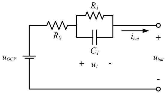
Figure 1.
First-order ECM. is the OCV, is the voltage at the battery terminals and is the voltage at the RC net.
Figure 1.
First-order ECM. is the OCV, is the voltage at the battery terminals and is the voltage at the RC net.

When analysing the circuit in Figure 1, the equations that describe it can be written as:
To ease the observer design process, it is convenient to rewrite (1) using the state-space formalism. Let the states be defined as follows
or in a more amenable form
Notice that states and are considered constant. This is a reasonable assumption, as these variables change because of the ageing of the battery, which happens over long time scales. Moreover, changes due to temperature variation are usually slow enough relative to the electrical time scale.
To summarise, the model presented in (3) presents only one known parameter, with a single input (the battery current) and a single output (the battery voltage).
2.2. Estimation Objective
The model presented in Section 2.1 does not have any directly measurable state. Moreover, the model is time-varying (as it depends on ), and the only measurable signals are the output () and the input . Thus, these two measurements need to provide enough information to perform the estimation of the four states. Thus, the estimation objective to generate an estimation of the states, , such that the following holds
where . In this estimation objective, we already assumed the effect that the presence of sensor noise and unknown parameters may have on the estimation accuracy.
We remark that, while it can be desirable to estimate the four states, it is the OCV one that the authors believe is more important. It has been mentioned that there is a direct relation between the OCV and the SoC, so if the OCV is estimated, SoC can be obtained, in the fashion of:
This relationship has been widely studied in the literature, with many models describing it. In [11,49] several OCV-SoC models are compared, while the review provided by [50] not only compares several models but provides some selection metrics and methods for the estimation of the parameters. Within the realm of OCV-SoC models, some of the most common ones include the Shepherd model, the Nernst model, a blend of both, as well as semi-empirical equations formulated using polynomial or exponential terms. In [49] these models can be found. Another common method is the use of look-up tables. We remark that the selection of the OCV-SoC model falls out of the scope of this document, but we encourage the reader to the referred literature if needed. Here, we consider that the knowledge that the two variables can be related is enough to proceed with the estimation of OCV.
2.3. Limiting Observability Assumptions of Existing Observers
Prior to any observer design, it is crucial to study whether the proposed estimation problem is solvable or not in the first place. Indeed, we need to analyse if the measured signal contains enough information in order to reconstruct the states of the system. In the control theory community, this type of study is known as observability analysis.
A system of the form (3) is said to be observable if any trajectory of the measured signal is generated by a unique initial condition of the system . Conversely, if there are multiple initial conditions of (3) that generate exactly the same output signal for all time, then the system is unobservable. A natural consequence of unobservability is that the state estimation problem cannot be solved.
We remark that the observability of the system (3) strongly depends on the current profile, , which is introduced on the battery. For instance, if we fix the current at a constant value , we can see that initial conditions and will generate the same output as the initial conditions and . Consequently, the proposed estimation problem can only be solved under particular current profiles. With this fact in mind, we motivate the necessity of explicitly studying the observability of the system (3). To do so, first, we consider the state transition matrix of the system (3) as the matrix that relates an initial condition of the system with the value of the states at time , ref. [51]
A well-known result from the literature ([51], Theorem 9.8) is that the initial condition will be uniquely determined by the measured signal y in the time interval if the observability Grammian is invertible. That is, the system (3) is observable if the current profile sufficiently excites the dynamics of the battery and guarantees that the Grammian is invertible.
This observability analysis is a well-known result in the control theory community; moreover, it has already been performed in similar equivalent circuit models, e.g., [45]. What is not that well known is that the convergence of the Kalman Filter (and its variances) requires a stricter condition known as uniform complete observability [52]. More precisely, the system (3) is uniform completely observable if there are some positive constants and such that, for all , the following is satisfied
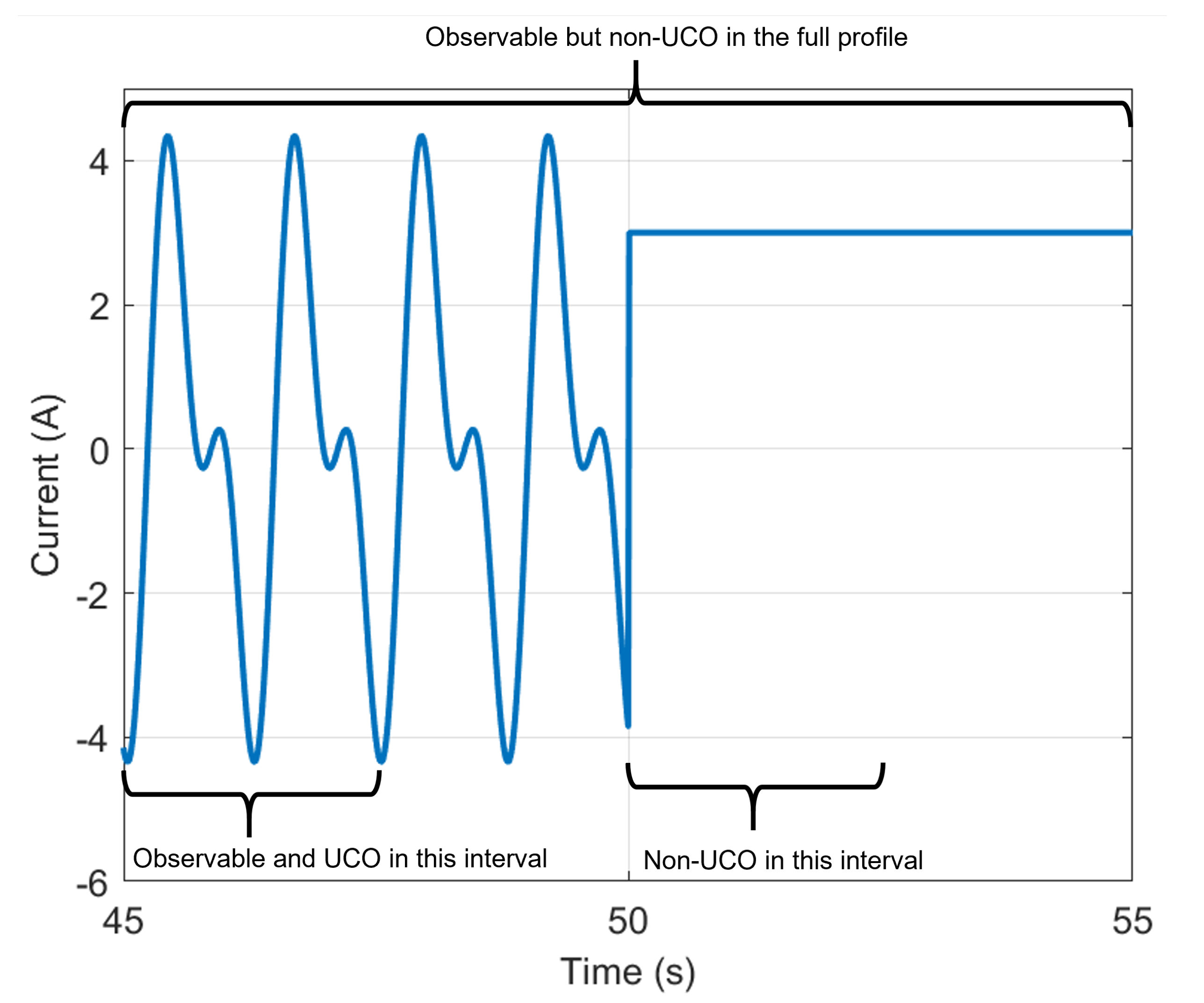
Although the definitions of observability and uniform complete observability are relatively similar, they present some technical differences with significant practical relevance. Precisely, the observability of the battery model (3) only needs to be satisfied in a finite window of time , while uniform complete observability needs to be satisfied persistently in time and in a fixed window defined by T. To better understand this difference, consider the current profile represented in Figure 2.
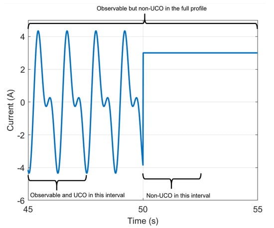
Figure 2.
Example of a current profile that makes the system observable but not Uniform Completely Observable (UCO). In the first 5 s, the profile excites the battery system in a way that makes the system observable and complies with UCO definition during this time-frame, but in the last 5 s, as the current is constant, the UCO condition is not met in this second time-frame. Consequently, because of the first part, this current profile ensures the observability of the battery during the whole 10 s while not guaranteeing UCO.
In this profile, during the first 5 s, the current is the sum of two sinusoidals, which is enough to guarantee observability and uniform complete observability in the time interval . Since this current profile makes the system observable during a specific time interval, the battery model will be observable during the full current profile. Nonetheless, after the second 50, the current is kept constant and the model stops being uniform completely observable. Therefore, even though the current profile in Figure 2 guarantees observability of the battery model, that is, the measured signals will contain enough information so as to estimate the unknown parameters, it does not guarantee uniform complete observability. Consequently, any Kalman filter implemented in a battery with this current profile is not guaranteed to converge.
We highlight that this difference between observability and uniform complete observability is of significant importance for Li-ion batteries and, to the best of our knowledge, has been missed in the estimation literature. Indeed, the importance of this difference is twofold. First, most estimation results in equivalent circuit models focus on Kalman Filters (and variations of the Kalman Filter) [29] which require uniform complete observability. Second, most Li-ion battery applications implement current with various excitation levels, for example, in vehicular applications, when the vehicle is stopped there is no excitation in the battery. Consequently, uniform complete observability is rarely satisfied in practice.
To solve this issue, in Section 3, and for the first time in the context of Li-ion batteries, we propose an observer that does not require uniform complete observability and has guaranteed convergence with the milder observability condition.
2.4. What If a Higher-Order Model Was Considered?
One may wonder what would happen if a higher-order model was considered. As a higher-order model would contain at least one more RC net, let us take a second-order model as an example, which adds another RC net to the circuit shown in Figure 1. A quick analysis shows that a second-order model with full unknown parameters is not observable. Precisely, it is not uniform completely observable and does not satisfy the interval excitation condition. We recall here that the system will be non-observable if there are multiple parameter values that generate an identical measured signal. Indeed, notice that if the parameter values of net 1 and net 2 were interchanged, the value of would be identical; therefore, it would be possible to achieve two solutions with the same exact output, without a way to determine which values are correct. Therefore, high-order ECM do not satisfy any minimal observability condition if the full parameters are completely unknown. In this sense, some information of the unknown parameters should be included for our technique to be implementable. Let us be reminded that the only measurable variables are and .
In relation to using different ECM, for instance, the work in [45] studies the observability of a different type of circuit and shows that UCO is only satisfied for particular current inputs. In this sense, our approach could relax the UCO property to one with weaker observability.
3. Proposal
This section is dedicated to presenting the main result of the paper. That is, we present an observer for the battery system which only requires a mild observability assumption. The observer is based on applying the ideas presented in [46] to the presented battery model in (3).
The main idea of the observer is, first, to transform the state-estimation problem into a parameter-estimation problem [53]. Second, the parameters are estimated through a parameter-estimator algorithm based on the recently proposed dynamic regressor extension and mixing (DREM) approach [54]; see [55] for a recent review on the topic. The combination of these two steps results in a estimator that relaxes the observability assumptions.
The next subsection is dedicated to explaining how the state estimation problem can be transformed into a parameter estimation one.
3.1. Transforming the Problem
Consider the battery model (3) and recall the definition of the state transition matrix in (6). The estimation objective described in Section 2.2. should also be considered Consider a copy of the battery model of the form
Notice that the solution of (9) can also be depicted through the state transition matrix (6). That is, . Since we do not know the initial condition of the battery, in general, we will have , which means that the copy (9) is initialised at a different initial condition from the ground-truth model (3).
Now, we define the error between the battery state and the copy model . Then, since both the battery model and the copy of the model are linear, the dynamics of the error can be computed through the same state-transition matrix. More specifically,
From this result, we can see that the states of the battery model can be computed as
where . Notice that the signal comes from the copy of the model (9), which can be run in parallel to the battery system; thus, is known. The state transition matrix can be computed by running in parallel the following equation
Therefore, the only thing that remains to be computed is the unknown parameter (that is, a constant value) vector related to the initial error between and . In other words, if we are able to estimate , we can reconstruct the states through (11). From this, we can see how the state estimation problem can be transformed into a parameter estimation one.
The next natural question is how to estimate the parameter . Indeed, from (11), we can deduce the following equality
which can be rearranged as the following linear regression equation
where and . Notice that both and are measurable signals; thus, what remains is exploiting these measurable signals and the linear regression Equation (14) in order to estimate the unknown parameter . This will be the focus of the next section.
3.2. Estimator Equations
There are plenty of existing algorithms that can be utilised to solve the parameter estimation problem in (14). Some notable examples are the gradient descent [44]; the least-squares algorithm [56], with its variations; or high-order algorithms [57,58], as well as the adaptive parameter estimator of [43]. Nonetheless, the convergence of all these algorithms requires what is usually referred to as a persistence of excitation condition. Indeed, we say that the linear regression in (14) satisfies the persistence of excitation condition if there exist some positive constants and such that
Roughly speaking, the persistence of excitation condition is related to the fact that the signal should contain enough information to infer the parameters . Nonetheless, by recalling the definition of , we can see that persistence of excitation the linear regression (15) is equivalent to uniform complete observability of the original system (8). Consequently, if we just implemented classical parameter estimation algorithms in (14), we would be unable to solve the observability conflict described in the past section. For this reason, this section proposes using a parameter estimator based on the DREM idea [55]. Specifically, we propose using the algorithm presented in [54], which has been proven to converge under milder observability conditions and has already been used to relax the persistence of excitation condition in other electrochemical devices [59].
The general idea of the algorithm in [54] is to pass the measured signals and through a set of pre-processing dynamics and then compute a nonlinear adjugate operation over the post-processed signals. Then, a standard gradient descent is implemented over the resulting signals. More precisely, the structure of the estimator is as follows:
where and are positive constants to be tuned and
where and refer to the determinant and adjugate of a matrix.
Intuitively, the main idea of the proposed observer is to introduce the measured signals and to the pre-processing dynamics and in (16) and then compute the nonlinear operations in (17) in order to generate the new signals and . Then, even if the original measured signals and did not present a persistence of excitation condition, the new signals and may indeed present such a condition. This allows the parameters to be recovered through the dynamics in (16).
More precisely, in [54], it was proven that such an estimator has guaranteed convergence if the linear regression in (14) satisfies an interval excitation condition. That is, for a positive constant , the following matrix
is invertible. Notice that interval excitation of the linear regression (14) is equivalent to the observability of the original system (3) as presented in the past section. Therefore, by implementing (16) in the considered system, for the first time, we can relax the uniform complete observability to a milder observability condition and still guarantee estimation convergence.
4. Numerical Simulations
4.1. Methodology
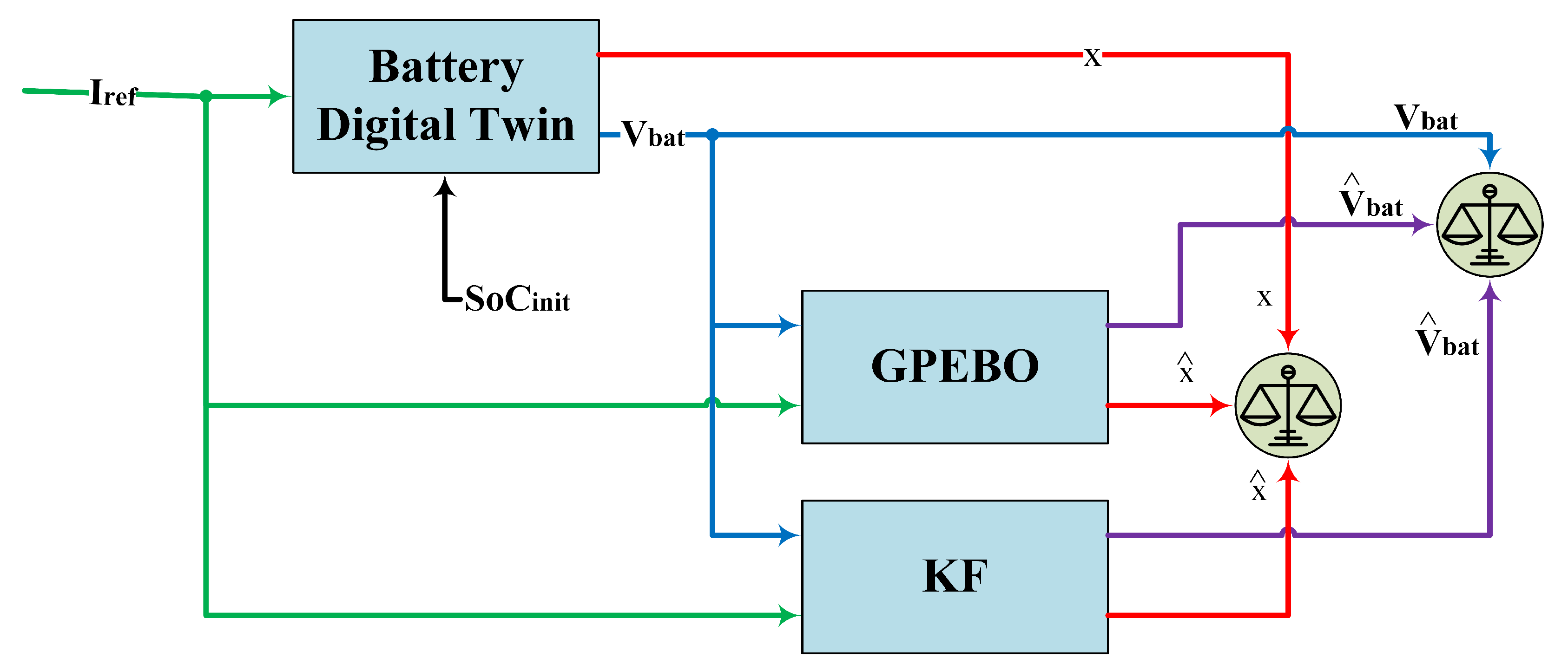
In order to analyse the effectiveness of the formulated observer, a series of numerical tests were developed. To perform this analysis, a digital twin of a real lithium-ion battery system was considered, which allowed us to mimic the expected measurable battery voltage, which was used, together with battery current, as input for the observers. Later, the estimated battery voltage was compared with the measured one, as well as the estimated states are compared to those of the digital twin. The battery current varied depending on the test performed. This can be seen in Figure 3.

Figure 3.
Simulation diagram.
The digital twin is based on the lithium-iron phosphate (LFP) battery provided by [47], and its specifications are presented in Table 2. The main reason to use this work is that it provides a first-order model that has been calibrated and validated, making it possible to have a realistic idea of the values that the different parameters , and can take in real applications. These parameters were estimated for different SoC levels, but for our work case, they are considered constant and independent of the SoC. Therefore, the values that have been considered correspond to the average of all SoC level values, obtaining the following parameters for the first-order model:
Table 2.
Lithium-iron phosphate (LFP) battery specifications. Extracted from [47].
With this model in mind, we develop different studies in order to see if the observer is capable of correctly estimating the parameters defined in (19), which from now on will be referred to as the real parameters.
In order to see the advantages of the proposed observer, it will be compared with the common and well-known Kalman filter (KF) technique. Furthermore, for a more exhaustive study, different scenarios will be considered.
The first case that has been analysed is one in which the current profile guarantees persistent excitation of the battery model. In this scenario, both observers should present good performance results. In the second case, a case of non-persistent excitation is studied in which better behaviour of the GPEBO should be observed with respect to the KF one. Finally, three more scenarios are considered which attempt to contemplate different phenomena or operating situations, such as the measurement noise phenomenon, the effect of not considering the OCV constant and the use of load profiles that may be demanded in real applications, such as Worldwide Harmonised Light Vehicles Test Procedure (WLTP).
All these experiments have been performed assuming that the value of the product between the resistor and the capacitor is known; that is, the parameter in (3) is known, in order to test an ideal case in which both observers should achieve satisfactory estimation. The product between and , for this particular case of study, is 95.5431 . Hence, in Equation (3) acquires the value of 0.010469. The reason behind the selection of KF as a benchmark is that KF-based algorithms are very popular in the literature. We have used the basic KF because the model (1) is linear. Even though batteries are non-linear systems, the description used is that of a time-varying linear system. EKF is suitable for linearising non-linear systems and treating them in a linear way, but if we applied it, the result would be the same as KF, as the linearised-model would be the already-linear model we have considered. A different situation happens regarding SMO or other non-linear observers. Based on our knowledge, utilising non-linear observers in linear systems often results in a poorer performance than utilising a linear observer. For the particular case of SMO, the high order of the model would result in too-high sensibility to noise, which would greatly affect the estimation.
The equations of KF are as follows:
where P is the state covariance matrix, R is the measurement covariance matrix and Q is the process noise covariance matrix.
Finally, for each of the studied cases, two different tunings have been tested for each observation. We establish as the KF gain and as the GPEBO gain. First of all, let it be noted that is not a gain itself, but an adjustment of the covariance matrix of the noise of the KF. A larger covariance matrix will, in most of cases, produce a more robust filter but at the expense of the convergence time. is obtained following Kalman’s procedure and only depends on the characteristics of the noise. On the other hand, is purely a gain parameter. The tuning of this parameter is a trade-off between sensibility to noise and convergence time. As can be seen, both observers have very different tuning processes, which make comparison difficult. Therefore, it is not possible to establish a solid criteria regarding which gain is high or low, as the magnitude is relative.
4.2. Case 1: Persistence of Excitation Current Signal
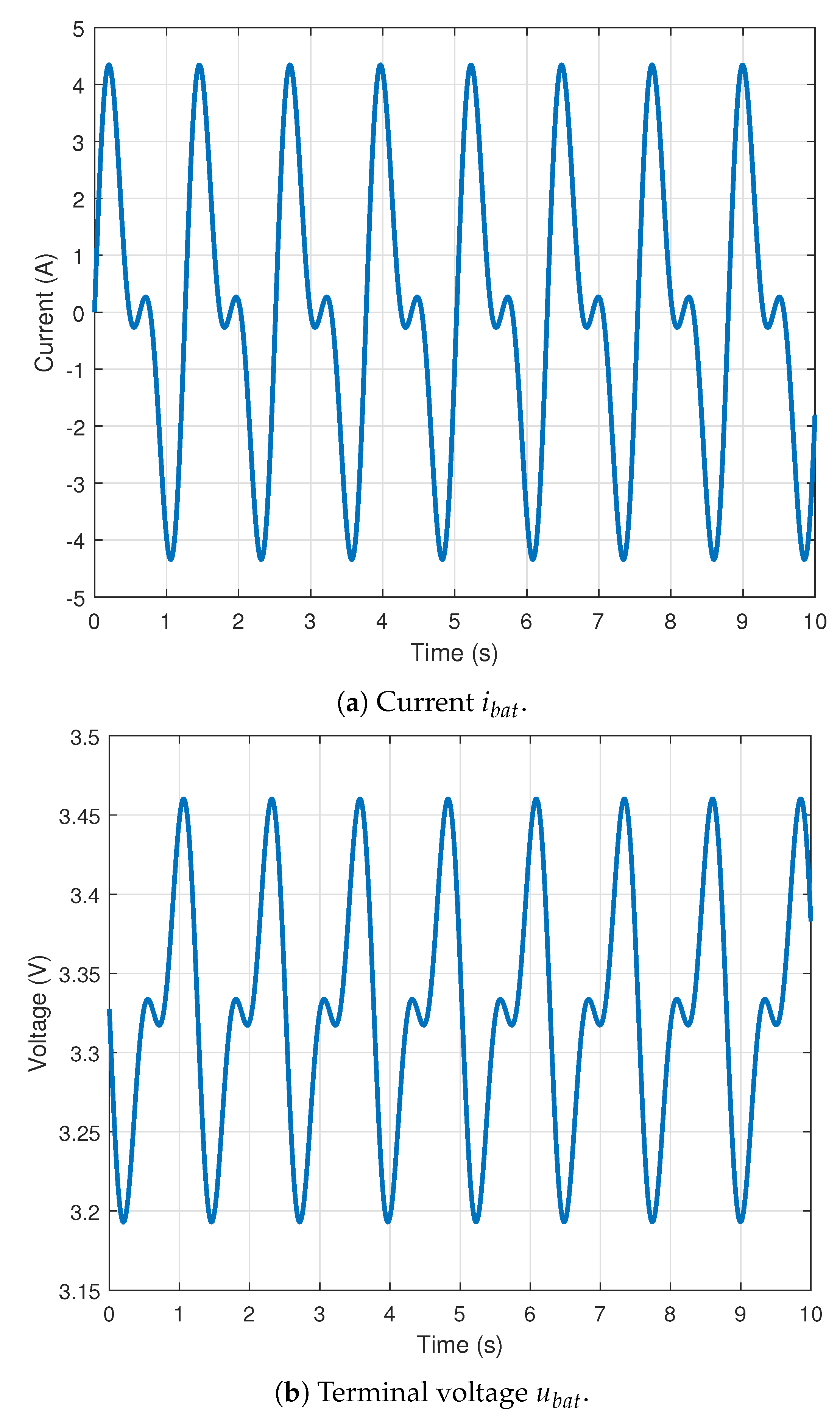
The first experiment consists of the estimation of the OCV (denoted by in the statement problem written in (2)) under an input current that guarantees persistence of excitation. To ensure this condition of persistent excitation, different sinusoidal signals have been used, resulting in the current profile that can be seen in Figure 4a.
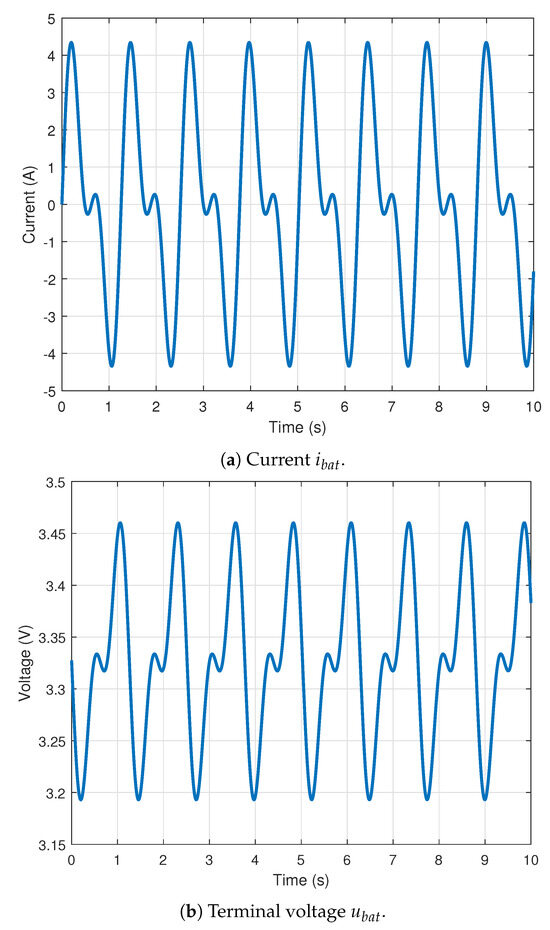
Figure 4.
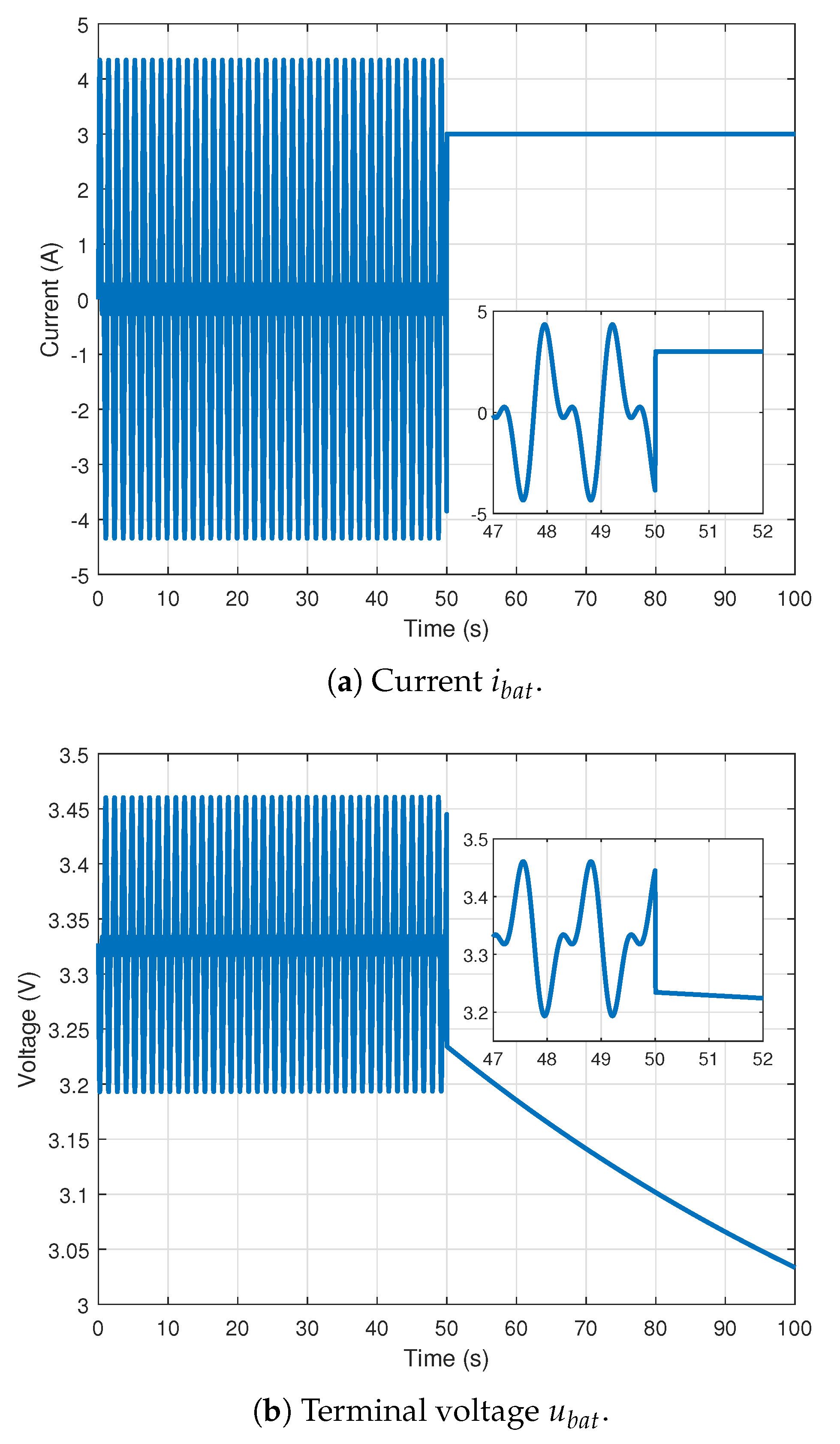
Current and terminal voltage profiles used to guarantee the persistence of excitation condition. the current is a custom profile defined by two sinusoidal signals of amplitude 2 and 3 A, and 10 and 5 Hz of frequency, respectively. The terminal voltage response is calculated according to this current profile and the model described in (1).
Considering this current, a constant OCV of 3.3275 V and the system parameters defined in (19), the resulting terminal voltage can be computed by means of the first-order model defined in (1). The profile of this terminal voltage is shown in Figure 4b, in which it is possible to see the effect of the ohmic resistor and the RC net.
Using this current profile, a simulation in MATLAB was launched simultaneously with both KF and GPEBO observers to estimate the OCV state starting from null initial conditions. The KF observer was computed in its classical form according to [60], tuning the covariance matrix of the process noise . This covariance matrix was defined by means of the identity matrix multiplied by an observer gain defined as . With respect to the GPEBO observer with the structure presented in (16), it was programmed in MATLAB to tune the observer gain .
The results obtained can be observed in Figure 5, in which it is possible to see how the estimated OCV converges to the real value in both cases. Looking at these profiles, it is possible to state that the GPEBO converges uniformly to the real value, while the KF estimation does not present this behaviour. These results fit with the theory explained in Section 3.

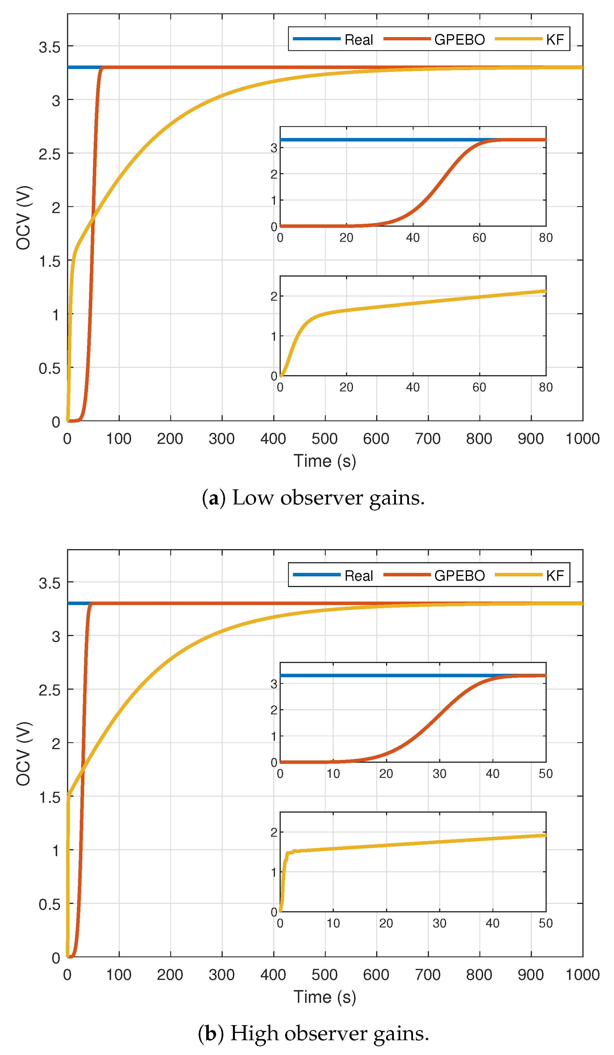
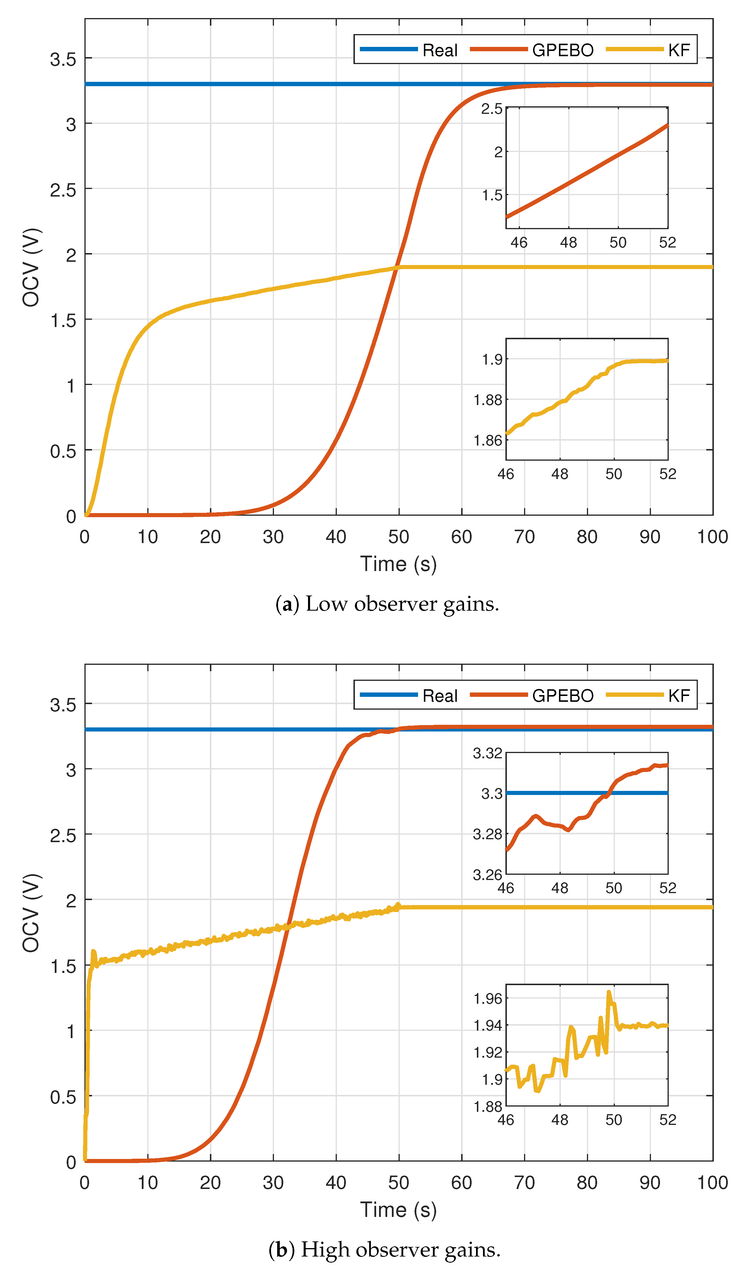
Figure 5.
Profiles of the real and estimated OCV using the KF and GPEBO for different gain observers for the persistent excitation profile shown in Figure 4. (a) Using low observer gains of = 0.005 and = 0.1. (b) Using high observer gains of = 5 and = 100.
On one hand, the KF ensures the convergence of the full parameter vector, creating a dependence between the individual elements. Therefore, it is possible to find parameters that converge with non-uniform behaviours according to the observer gains. This behaviour can be observed in the details of the KF profiles (in yellow) in Figure 5. As can be noticed, firstly, the estimated OCV increases from 0 V to 1.5 V in less than 10 s to later change the profile until the estimation converges to the real value at 700 s. Moreover, it can be seen that the time required to reach this initial point of 1.5 V is directly related to the observer gains. Using a of 0.005, the observer requires 10 s to reach the 1.5 V as can be seen in detail in Figure 5a, while this time is reduced until 1 s using a of 5, as seen in detail in Figure 5b. At this point, it is important to notice that the value of does not guarantee that all parameters will converge to the real values in a shorter or longer period of time. Looking at both Figure 5a,b it can be noted that the OCV converges to the real value at 700 s independently from the observer gain .
On the other hand, using the GPEBO proposed in this work, the behaviour of the observed dynamics is totally different. For this particular case, each parameter converges independently from the others following a uniform profile. This property can be observed in the details of Figure 5a,b that show the profiles of the OCV estimated by means of the GPEBO in red. Furthermore, for this observer the gain has a direct impact on the convergence time, making it possible to decrease the convergence time increasing the observer gain . Figure 5a shows the OCV profile using a value of = 0.1, where it is possible to see how the OCV converges to the real value in 60 s. This convergence time can be reduced using a greater value of , as can be noticed in Figure 5b where the convergence time is 40 s with = 100.
At this point, it can be concluded that under the condition of persistent excitation, classical techniques such as the KF observer works properly but do not allow a direct tuning of the convergence time. In counterpart, the GPEBO presented in this work has the advantage of satisfying these requirements while guaranteeing a correct estimation of the parameters.
4.3. Case 2: Non-Persistence of Excitation Current Signal
The second experiment that was carried out used a current profile which presents an interval that is not UCO, followed by the example presented in Figure 2 of the previous section.
The current profile selected consists of the same one used in the previous case, but introduces an interval of constant current of 3 A. This current profile can be seen in the following Figure 6a, while the terminal voltage of the battery considering this current appears in Figure 6b.

Figure 6.
Current and terminal voltage profiles used to analyse the problem of a non-persistence excitation condition. Current is a custom profile that defined the first 50 s using two sinusoidal signals of amplitude 2 and 3 A, and 10 and 5 Hz of frequency, respectively, and the remaining time by a constant value of 3 A. The terminal voltage response is calculated according to this current profile and the model described in (1).
In order to see the performance of the GPEBO observer under the operating condition of non persistent excitation, we used the observer gain = 0.1, which was small, to ensure that the required estimation time was greater than 60 s. For the case of the KF observer, we used a gain = 0.005.
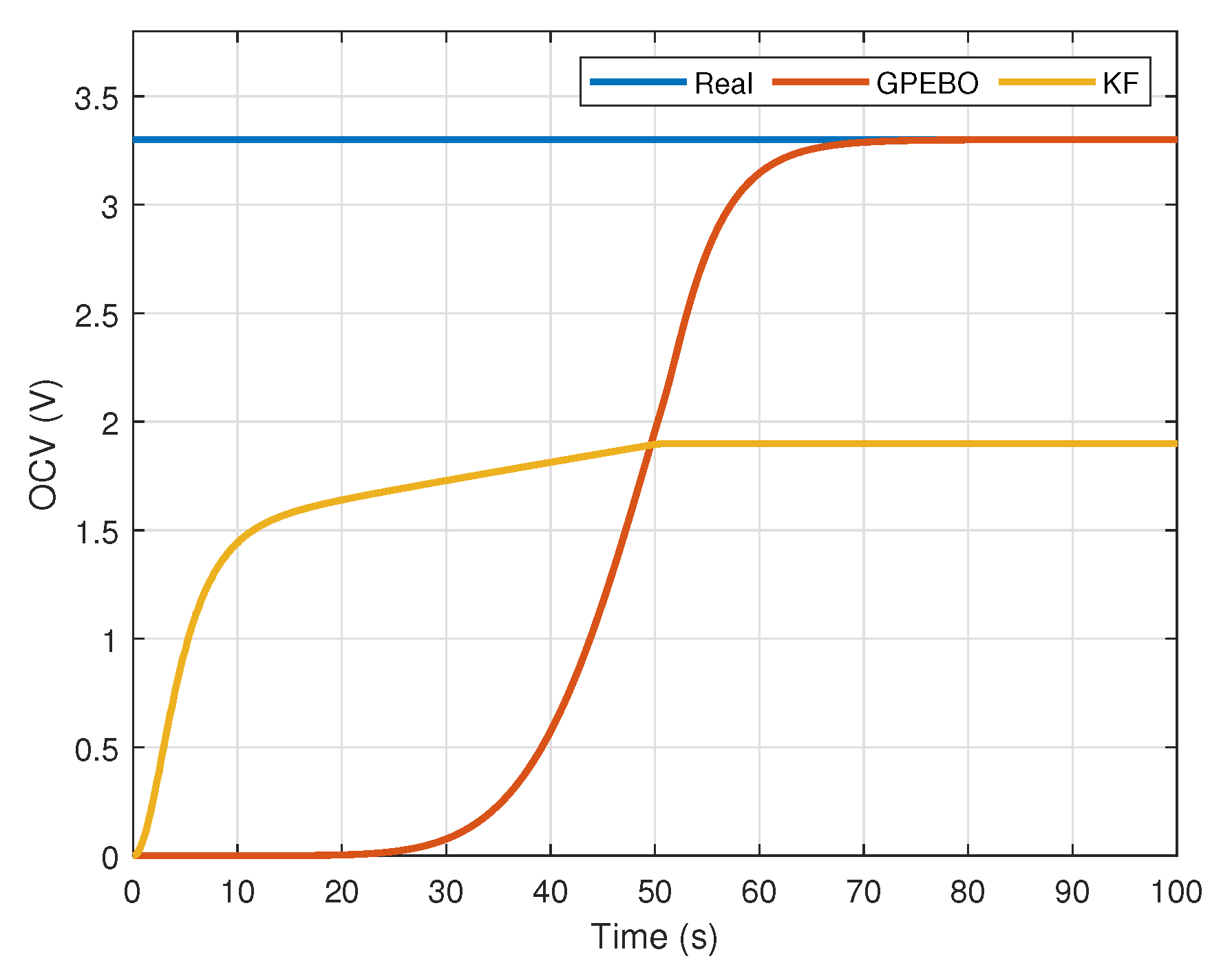
As can be seen in Figure 7, in the moment in which the observable profile is interrupted, KF stops converging and the value of the estimated OCV remains constant with an important error with respect to the real value. For the case of the GPEBO, it converges to the real OCV without any apparent effect. As shown, the OCV approaches the real value from the second 70, although the constant current appeared 20 s earlier. Moreover, it should be highlighted that the estimated OCV follows its characteristic uniform profile.

Figure 7.
Profiles of the real and estimated OCV using the KF and GPEBO using the non-persistent excitation profile presented in Figure 6.
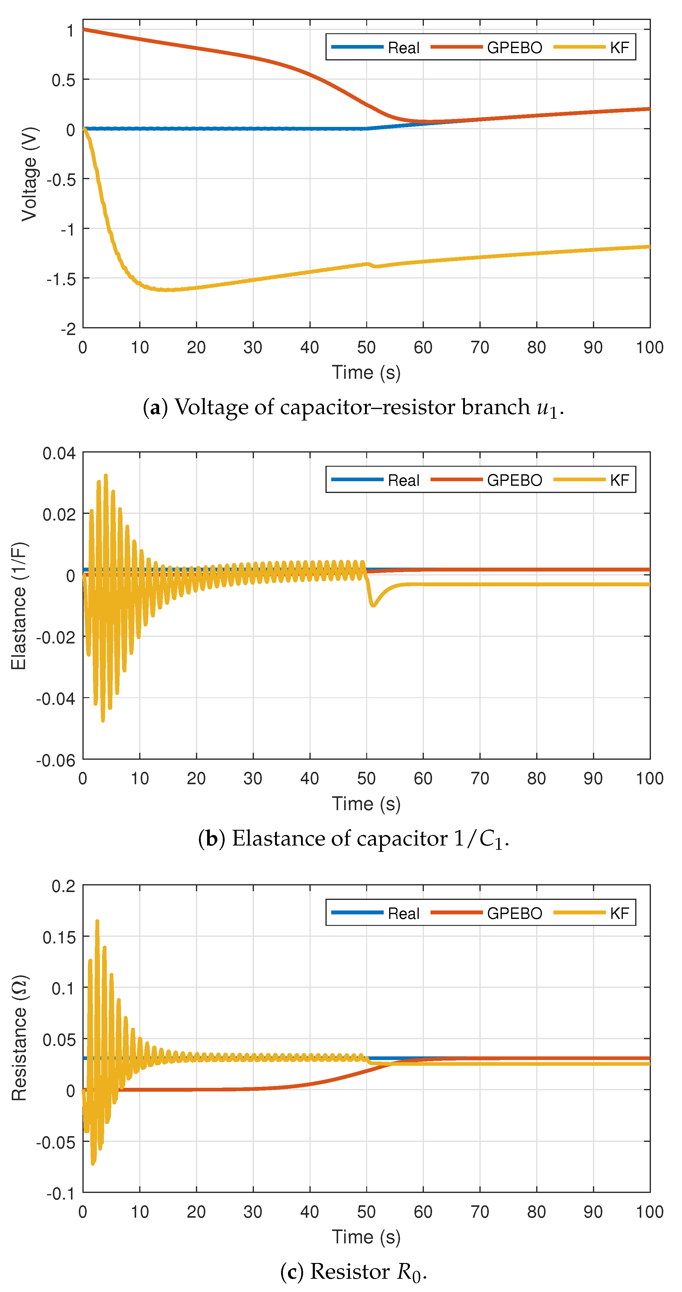
Using this experiment has made it possible to validate the correctness of the proposed observer while taking the other states into account. Taking into account the model described in (3), aside from the the OCV state, there are three more states that can be estimated. The first is the voltage in the capacitor–resistor branch, which is denoted as . The second is the inverse of the capacitor value , which can be defined as elastance and expressed in units of 1/F. The final state is the resistor , which is connected in series with the capacitor-resistor branch.
Figure 8 presents the evolution of these different states mentioned. In this figure, it is possible to see how, by means of the GPEBO, it is possible to estimate their correct values.
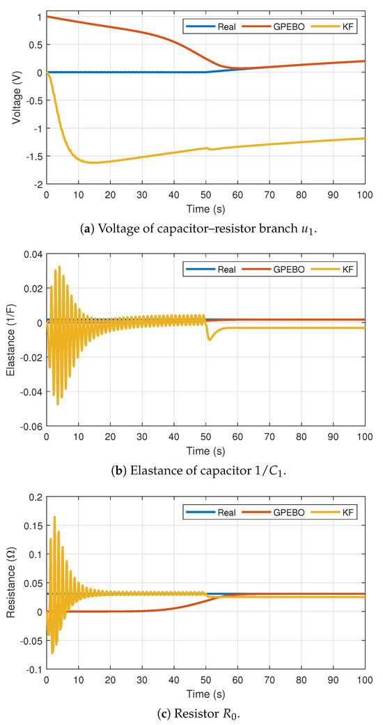
Figure 8.
Profiles of the real and estimated states using the KF and GPEBO using the non-persistent excitation profile presented in Figure 6. (a) Voltage of the resistor-capacitor branch . (b) Elastance (inverse of capacity) of the condensator . (c) Resistance of the series resistor .
Using this study, it is possible to highlight the advantage of the proposed observer with respect to classical ones, when battery operating conditions with non-UCO profiles are used. In future studies, in order to simplify the analysis, only the estimation result of the OCV state, which is directly related to the SoC of the battery, will be presented.
4.4. Case 3: Sensor Noise
The next study that was developed consists of introducing measurement noise in the output signal. Thus, a distributed Gaussian random signal with 0 mean and 0.001 variance has been introduced to the profile.
To perform this first scenario, the same current profile from the previous study was used, which corresponds to a sinusoidal current with a not UCO interval as can be seen in Figure 6a. Using this current and the measurement noise mentioned, the obtained signal is the one shown in Figure 9.
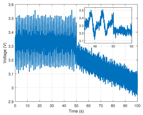
Figure 9.
Terminal voltage considering the current profile shown in Figure 6a and a Gaussian random measurement noise with 0 mean and 0.01 variance.
In order to see the effect of the measurement noise and how, by means of the observer gains, it can be reduced, different values of the observer parameter gains and were used. The values chosen are the same ones from the first study, in which two different were considered for the GPEBO, which correspond to 0.1 and 100, while the values for the KF observer are 0.005 and 5. Figure 10 presents the estimated OCV for both GPEBO and KF observers under the conditions of measurement noise described.
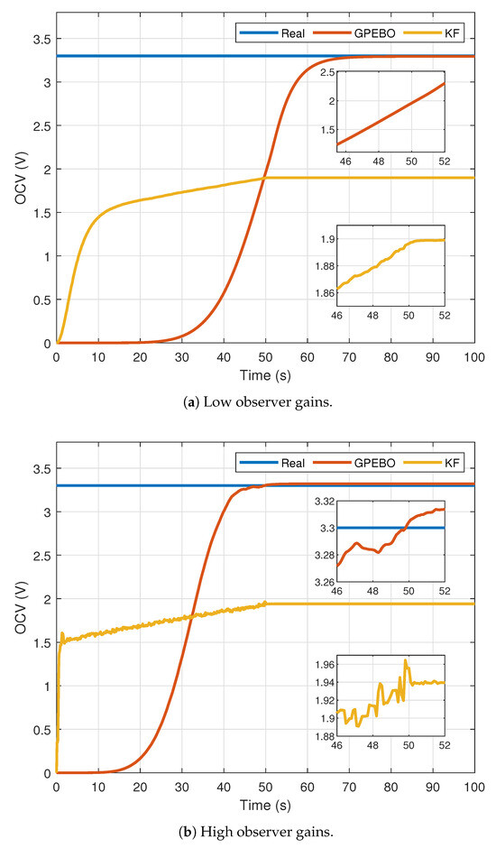
Figure 10.
Profiles of the real and estimated OCV using the KF and GPEBO for different gain observers considering the noise output measurement shown in Figure 9. (a) Using low observer gains of = 0.005 and = 0.1. (b) Using high observer gains of = 5 and = 100.
As can be noticed in Figure 10a, using a low gain = 0.1 for the GPEBO, the OCV converges to the real value following a uniform profile without noise. With respect to the KF, using a = 0.005, it is possible to observe how stills do not converge to the real value when the non-UCO interval appears. Moreover, in the same time window used in the details of both KF and GPEBO profiles, it is possible to note how the OCV estimation for the case of the KF method presents significant noise.
If a higher-value parameter for the GPEBO is used, the estimation presents more noise along its profile and it is possible that it does not converge to the exact real value. This behaviour can be seen in Figure 10b using = 100. As can be observed, although the estimated OCV tries to converge more rapidly to the exact value, it finally presents a constant error which, despite not being very high, must have been taken into account. With respect to the KF results, introducing a gain = 5, it is possible to highlight the increase in the noise in the OCV estimation, compared to the previous low gain used.
Taking into account these results, it is clear that, as in the vast majority of observers, there is a trade-off between the convergence time and the sensibility to measurement noise. For the case of the GPEBO, the analysis shows that a small value must be selected in order to guarantee that the estimation will converge to the real value with null error. Concerning the KF observer, it is clear that due to the presence of a non-UCO interval, the estimation does not converge to the real value, but the influence of the measurement noise can be counteracted by decreasing the value of .
4.5. Case 4: Variable OCV
An important study that must be developed is one that analyses the behaviour of the observer when the OCV (directly related to the SoC) varies. According to the model presented in (3), the OCV is considered as a constant parameter. In this context, an adequate observer should be robust to this discrepancy between the reality and the model.
In order to perform this analysis, a different case from the previous experiments was considered. Indeed, instead of assuming a constant OCC, a sinusoidal OCV was used, in order to ensure that the battery remained in its operational region in search of a realistic scenario.
Similar to the previous experiment, the same observer gains were used for both GPEBO and KF observers in order to analyse their effect on the estimation performance. Figure 11 shows the results obtained for this experiment when the persistent excitation current shown in Figure 4a is used.
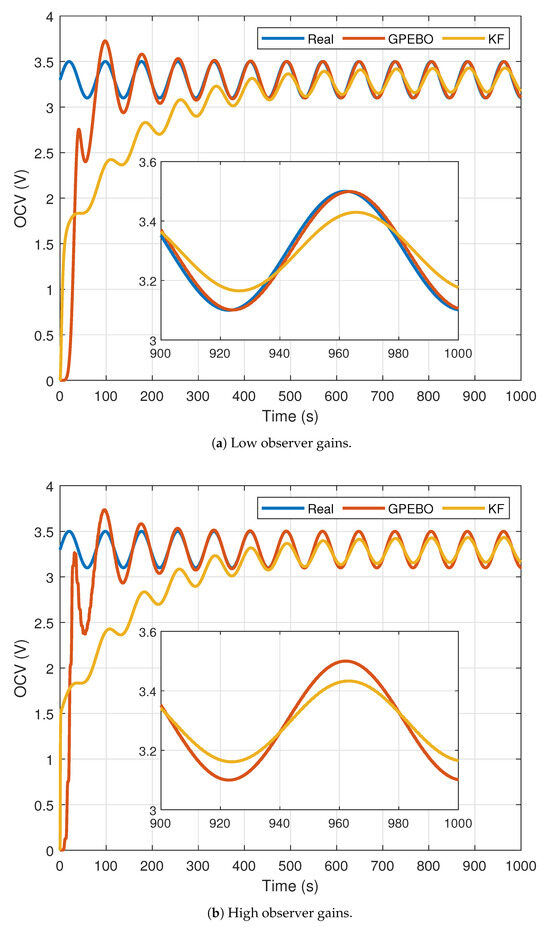
Figure 11.
Profiles of the real and estimated OCV using the KF and GPEBO for different gain observers when the OCV is not constant and is defined by means of a sinusoidal signal of 0.2 V amplitude, 3.3 V mean value and 0.08 Hz of frequency. (a) Using low observer gains of = 0.005 and = 0.1. (b) Using high observer gains of = 5 and = 100.
As can be noticed, the use of the GPEBO makes it possible to estimate the real OCV with practically null error when steady-state behaviour occurs. Using an observer gain = 0.1, the detail of Figure 11a shows the existence of a very small error between the real value and the estimated one. This error disappears when a higher value of is used, as shown in further detail in Figure 11b.
It is important to remark that the use of the KF does not guarantee the convergence of the observer to the real value of OCV. Although a persistent excitation profile for the current signal is used, the observer is not able to estimate the OCV with null error when it changes over time. For this particular case, the only effect of the observer gain is to push the estimation more quickly or more slowly at the beginning of the experiment, as seen in the first experiment carried out in Section 4.2.
4.6. Case 5: Vehicle Load Profile
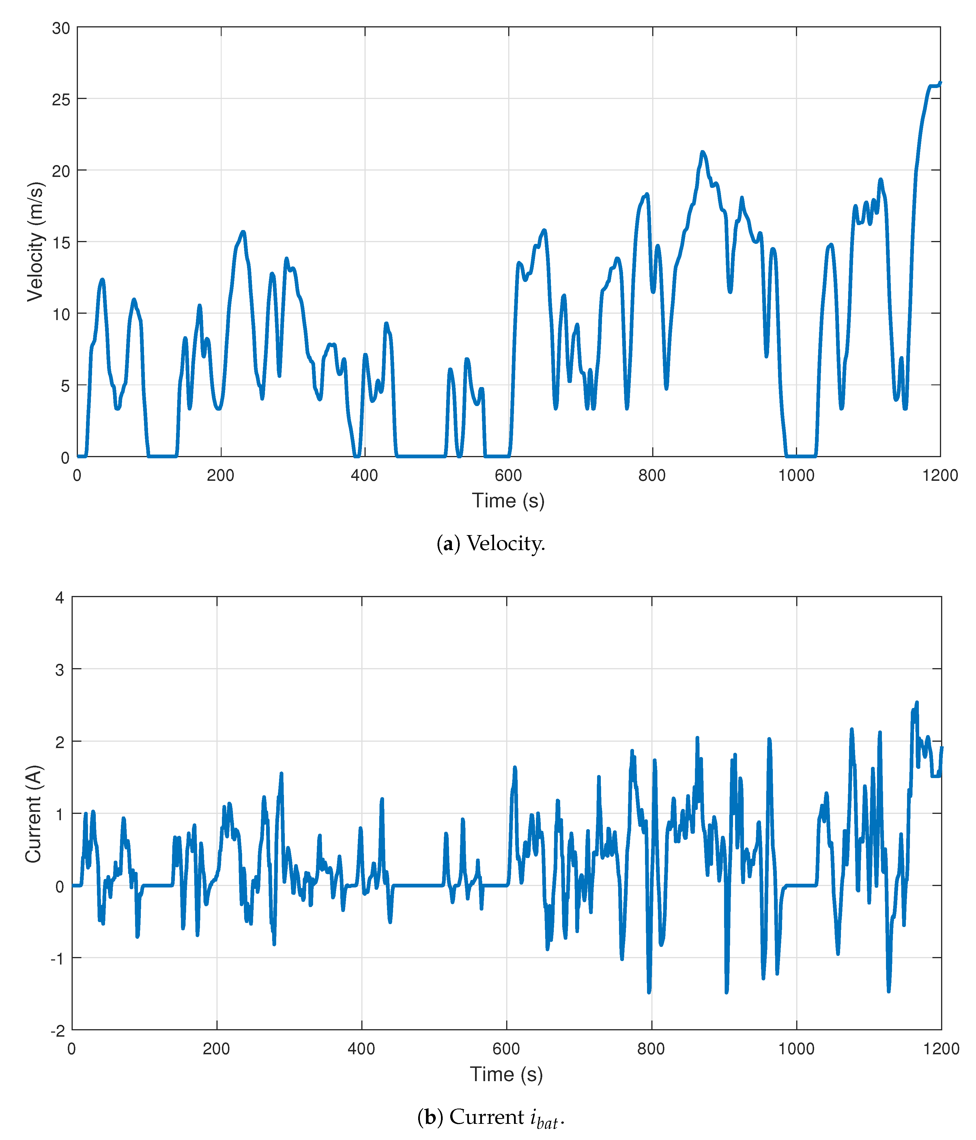
As has been mentioned, one of the points of this work is to guarantee the state and parameter estimation of lithium-ion batteries under real operating conditions. For that reason, in the last-case scenario, the load profile proposed is a standard driving cycle WLTP, which is used to test range, fuel consumption, and emissions in light vehicles in the European Union. It applies mainly to passenger cars, vans, and some buses. For our case study, the load profile used has been extracted from the velocity profile of the WLTP driving cycle [61,62], which can be observed in Figure 12a. From this velocity, it is possible to obtain the current profile according to the model and parameters that define the dynamics of a vehicle ([63], Chapter 7); for instance, the Toyota Proace 50 kWh model [64]. Finally, the current has been scaled using a factor 1/5000 to meet the requirements of the lithium-ion battery defined in Table 2. The profile of this scaled current can be seen in Figure 12b.
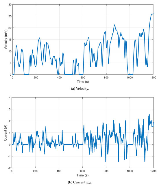
Figure 12.
Velocity and current profiles of the WLTP driving cycle [61]. This profile has been scaled and transformed to current using the equation of the vehicle dynamics [63].
Using this current profile, a simulation has been launched that considers the OCV as constant in order to study if the observer can estimate its value. As can be noticed in Figure 12b, this current profile has some regions with constant null values. Thus, it is interesting to analyse how the observer behaves under this situation.
Following with the same procedure developed in previous experiments, the same sets of observer gains were tested again, showing different performances depending on the gain values. Figure 13 shows the OCV estimations considering the low and high observer gains. As can be noticed, the use of the GPEBO correctly estimates the OCV with null error, while for the case of the KF, it does not reach the ground-truth value.
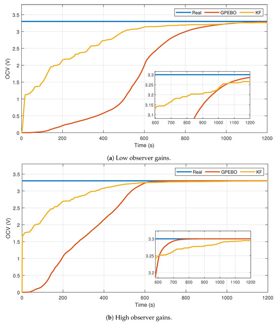
Figure 13.
Profiles of the real and estimated OCV using the KF and GPEBO for different gain observers using the current profile shown in Figure 12b. (a) Using low observer gains of = 0.005 and = 0.1. (b) Using high observer gains of = 5 and = 100.
It is possible to see how the KF observer does not converge to the real value of OCV according to the details shown in Figure 13a,b, which correspond to the low and high observer gains, respectively. With respect to the GPEBO, it can be seen how, by means of a high observer gain = 100, the estimated OCV converges to the real one with null steady state error. However, with a low gain = 0.1, it is possible to see how there is a small error due to the fact that the estimation has not reached the steady state. Thus, it can be seen how a properly tuned GPEBO successfully estimates the real value, even though the convergence time is not short, when a realistic profile of the current is considered for the battery.
One may wonder why, in this case, KF seems to converge faster than GPEBO, even if the latter converges to the true value and KF does not. The reason behind this is that GPEBO includes two dynamical systems that are connected in the cascade. The first is -dynamics, which pre-process the measured signals. Second is the -dynamics, which use the post-process signals to estimate the parameters. In this sense, intuitively, the GPEBO requires the to reach a large enough value for the -dynamics to start quickly converging to the true value. This happens around 500 s in Figure 13a. Alternatively, the KF includes a set of dynamics (the -dynamics and the P dynamics) which run in parallel. Since the GPEBO has dynamics in cascade and the KF in parallel, the KF presents faster convergence during the initial times. A simple way of solving this is to initialise at a larger value in order to reduce the convergence time of the -dynamics. Nonetheless, in this work, we considered the worst-case scenario, in which we have no information regarding how to initialise this variable, so we initialise it at an arbitrary value of zero.
5. Conclusions and Future Work
In this document, a new SoC estimator has been developed based on the application of GPEBO, in a novel approach that merges the benefits of using a well-known, popular and linear model such as first-order ECM with an observer that guarantees accurate estimation even in the absence of persistent excitation.
It has been shown how, for the case with persistence of excitation, GPEBO works better than KF and for the non-persistence of excitation situation, KF is unable to converge, while GPEBO is not affected by the change in excitation. This performance is maintained when measurement noise is introduced, but in this situation, the gain needs finer tuning. A similar situation happens when the WLTP, a real profile, is introduced as a load to the battery. Again, KF is unable to converge but the GPEBO is highly dependent on the gains. Finally, for the case of a varying SoC, which is implemented through a sinusoidal variation of OCV, an analogue response is found, with an incapable KF and a capable GPEBO with a performance affected by gain. As a summary, it can be stated that in general, for an application such as the one considered, GPEBO works better than KF.
However, as shown by the simulation results, the tuning of the GPEBO is not trivial and requires careful treatment. On the other hand, once properly tuned, it performed successfully in all the experiments, showing its advantages against KF, which was used as a benchmark.
Considering these points, some future lines of research appear to be interesting:
- Test of the performance against full unknown parameters. In the test performed, the time constant of the circuit, , was assumed to be known. We think that practical applications would benefit if the GPEBO did not need to know this parameter.
- Experimental validation. Independent test to characterise the cell (as in [48]) to compare it against the estimated value of the parameters.
- Experiment with temperature sensitivity. With temperature affecting the value of many ECM parameters, it would be interesting to test the performance of GPEBO with different temperatures.
- Automatic tuning. Automatic tuning would solve the main drawback that we have experienced, which is finding a gain that ensures performance.
Author Contributions
Conceptualisation, A.C. (Andreu Cecilia), A.C. (Alejandro Clemente) and M.M.-F.; methodology, M.M.-F., A.C. (Andreu Cecilia) and A.C. (Alejandro Clemente); investigation, A.C. (Alejandro Clemente), M.M.-F. and A.C. (Andreu Cecilia); writing—original draft preparation, M.M.-F., A.C. (Alejandro Clemente) and A.C. (Andreu Cecilia); writing—review and editing, R.C.-C., A.C. (Andreu Cecilia) and A.C. (Alejandro Clemente); visualisation, A.C. (Alejandro Clemente), M.M.-F. and A.C. (Andreu Cecilia); supervision, R.C.-C.; project administration, R.C.-C.; funding acquisition, R.C.-C. All authors have read and agreed to the published version of the manuscript.
Funding
This research received support from the Spanish Ministry of Science and Innovation under projects MAFALDA (PID2021-126001OBC31 funded by MCIN/AEI/10.13039/501100011033/ ERDF,EU) This work is part of the project MASHED (TED2021-129927B-I00), funded by MCIN/ AEI/10.13039/501100011033 and by the European Union Next GenerationEU/PRTR. This research was funded by FI Joan Oró grant (code 2023 FI-1 00827), cofinanced by the European Union.
Data Availability Statement
Data is contained within the article or openly available in [61].
Conflicts of Interest
The authors declare no conflict of interest.
Abbreviations
The following abbreviations are used in this manuscript:
| ANN | Artificial Neural Network |
| BMS | Battery Monitoring System |
| DFN | Doyle-Fuller-Newman |
| DREM | dynamic regressor extension and mixing |
| ECM | equivalent circuit model |
| EKF | Extended Kalman Filter |
| ESS | Energy Storage System |
| EV | Electric Vehicle |
| GPEBO | Generalized Parameter Estimation-based Observers |
| HGO | High Gain Observer |
| KF | Kalman Filter |
| Li-ion | Lithium-Ion |
| LIBs | lithium-ion batteries |
| OCV | Open Circuit Voltage |
| SMO | Sliding mode observer |
| SoC | State of Charge |
| SPM | Single Particle Model |
| SVM | Support Vector Machine |
| UCO | Uniform Completely Observable |
| UKF | Unscented Kalman Filter |
| WLTP | Worldwide Harmonised Light Vehicles Test Procedure |
References
- IEA. Electric Vehicles. IEA. Available online: https://www.iea.org/energy-system/transport/electric-vehicles (accessed on 19 October 2023).
- Carignano, M.; Costa-Castelló, R. Toyota Mirai: Powertrain Model and Assessment of the Energy Management. IEEE Trans. Veh. Technol. 2023, 72, 7000–7010. [Google Scholar] [CrossRef]
- IEA. Renewables—Energy System. IEA. Available online: https://www.iea.org/energy-system/renewables (accessed on 19 October 2023).
- Tarascon, J.M.; Armand, M. Issues and challenges facing rechargeable lithium batteries. Nature 2001, 414, 359–367. [Google Scholar] [CrossRef]
- Asri, L.I.M.; Ariffin, W.N.S.F.W.; Zain, A.S.M.; Nordin, J.; Saad, N.S. Comparative Study of Energy Storage Systems (ESSs). J. Phys. Conf. Ser. 2021, 1962, 012035. [Google Scholar] [CrossRef]
- Lee, S.B.; Thiagarajan, R.S.; Subramanian, V.R.; Onori, S. Advanced Battery Management Systems: Modeling and Numerical Simulation for Control. In Proceedings of the 2022 American Control Conference (ACC), Atlanta, GA, USA, 8–10 June 2022; pp. 4403–4414. [Google Scholar]
- Cai, W.; Yan, C.; Yao, Y.X.; Xu, L.; Xu, R.; Jiang, L.L.; Huang, J.Q.; Zhang, Q. Rapid Lithium Diffusion in Order@Disorder Pathways for Fast-Charging Graphite Anodes. Small Struct. 2020, 1, 2000010. [Google Scholar] [CrossRef]
- Sun, C.; Ji, X.; Weng, S.; Li, R.; Huang, X.; Zhu, C.; Xiao, X.; Deng, T.; Fan, L.; Chen, L.; et al. 50C Fast-Charge Li-Ion Batteries using a Graphite Anode. Adv. Mater. 2022, 34, 2206020. [Google Scholar] [CrossRef]
- Yue, X.; Zhang, J.; Dong, Y.; Chen, Y.; Shi, Z.; Xu, X.; Li, X.; Liang, Z. Reversible Li Plating on Graphite Anodes through Electrolyte Engineering for Fast-Charging Batteries. Angew. Chem. Int. Ed. 2023, 62, e202302285. [Google Scholar] [CrossRef]
- Zheng, L.; Zhang, L.; Zhu, J.; Wang, G.; Jiang, J. Co-estimation of state-of-charge, capacity and resistance for lithium-ion batteries based on a high-fidelity electrochemical model. Appl. Energy 2016, 180, 424–434. [Google Scholar] [CrossRef]
- Weng, C.; Sun, J.; Peng, H. A unified open-circuit-voltage model of lithium-ion batteries for state-of-charge estimation and state-of-health monitoring. J. Power Sources 2014, 258, 228–237. [Google Scholar] [CrossRef]
- Pattipati, B.; Balasingam, B.; Avvari, G.V.; Pattipati, K.R.; Bar-Shalom, Y. Open circuit voltage characterization of lithium-ion batteries. J. Power Sources 2014, 269, 317–333. [Google Scholar] [CrossRef]
- Movassagh, K.; Raihan, A.; Balasingam, B.; Pattipati, K. A Critical Look at Coulomb Counting Approach for State of Charge Estimation in Batteries. Energies 2021, 14, 4074. [Google Scholar] [CrossRef]
- Sesidhar, D.V.S.R.; Badachi, C.; Green, R.C., II. A review on data-driven SOC estimation with Li-Ion batteries: Implementation methods & future aspirations. J. Energy Storage 2023, 72, 108420. [Google Scholar]
- Alazki, H.; Cortés-Vega, D.; García, P. Diseño robusto de un observador de perturbaciones con saturaciones: Aplicación al control de regulación de la glucosa en pacientes con diabetes tipo 1. Rev. Iberoam. Autom. Inform. Ind. 2023, 1–9. [Google Scholar] [CrossRef]
- Plett, G.L. Extended Kalman filtering for battery management systems of LiPB-based HEV battery packs: Part 3. State and parameter estimation. J. Power Sources 2004, 134, 277–292. [Google Scholar] [CrossRef]
- Hu, C.; Youn, B.D.; Chung, J. A multiscale framework with extended Kalman filter for lithium-ion battery SOC and capacity estimation. Appl. Energy 2012, 92, 694–704. [Google Scholar] [CrossRef]
- Liu, C.z.; Zhu, Q.; Li, L.; Liu, W.q.; Wang, L.Y.; Xiong, N.; Wang, X.y. A State of Charge Estimation Method Based on H∞ Observer for Switched Systems of Lithium-Ion Nickel–Manganese–Cobalt Batteries. IEEE Trans. Ind. Electron. 2017, 64, 8128–8137. [Google Scholar] [CrossRef]
- Sun, F.; Hu, X.; Zou, Y.; Li, S. Adaptive unscented Kalman filtering for state of charge estimation of a lithium-ion battery for electric vehicles. Energy 2011, 36, 3531–3540. [Google Scholar] [CrossRef]
- Huang, C.; Wang, Z.; Zhao, Z.; Wang, L.; Lai, C.S.; Wang, D. Robustness Evaluation of Extended and Unscented Kalman Filter for Battery State of Charge Estimation. IEEE Access 2018, 6, 27617–27628. [Google Scholar] [CrossRef]
- Wang, S.; Jia, X.; Takyi-Aninakwa, P.; Stroe, D.I.; Fernandez, C. Review—Optimized Particle Filtering Strategies for High-Accuracy State of Charge Estimation of LIBs. J. Electrochem. Soc. 2023, 170, 050514. [Google Scholar] [CrossRef]
- Kim, I.S. The novel state of charge estimation method for lithium battery using sliding mode observer. J. Power Sources 2006, 163, 584–590. [Google Scholar] [CrossRef]
- Chen, X.; Shen, W.; Cao, Z.; Kapoor, A. A novel approach for state of charge estimation based on adaptive switching gain sliding mode observer in electric vehicles. J. Power Sources 2014, 246, 667–678. [Google Scholar] [CrossRef]
- Anderson, J.L.; Moré, J.J.; Puleston, P.F.; Roda, V.; Costa-Castelló, R. Control Super-Twisting con adaptación basada en cruce por cero. Análisis de estabilidad y validación. Rev. Iberoam. Autom. Inform. Ind. 2022, 20, 104–114. [Google Scholar] [CrossRef]
- Mukhopadhyay, S.; Zhang, F. A high-gain adaptive observer for detecting Li-ion battery terminal voltage collapse. Automatica 2014, 50, 896–902. [Google Scholar] [CrossRef]
- Jenkins, B.; Krupadanam, A.; Annaswamy, A.M. Fast Adaptive Observers for Battery Management Systems. IEEE Trans. Control Syst. Technol. 2020, 28, 776–789. [Google Scholar] [CrossRef]
- Limoge, D.W.; Annaswamy, A.M. An Adaptive Observer Design for Real-Time Parameter Estimation in Lithium-Ion Batteries. IEEE Trans. Control Syst. Technol. 2020, 28, 505–520. [Google Scholar] [CrossRef]
- Blondel, P.; Postoyan, R.; Raël, S.; Benjamin, S.; Desprez, P. Nonlinear Circle-Criterion Observer Design for an Electrochemical Battery Model. IEEE Trans. Control Syst. Technol. 2019, 27, 889–897. [Google Scholar] [CrossRef]
- Martí-Florences, M.; Cecilia, A.; Costa-Castelló, R. Modelling and Estimation in Lithium-Ion Batteries: A Literature Review. Energies 2023, 16, 6846. [Google Scholar] [CrossRef]
- Ghaeminezhad, N.; Ouyang, Q.; Wei, J.; Xue, Y.; Wang, Z. Review on state of charge estimation techniques of lithium-ion batteries: A control-oriented approach. J. Energy Storage 2023, 72, 108707. [Google Scholar] [CrossRef]
- Clemente, A.; Costa-Castelló, R. Redox Flow Batteries: A Literature Review Oriented to Automatic Control. Energies 2020, 13, 4514. [Google Scholar] [CrossRef]
- Puleston, T.; Clemente, A.; Costa-Castelló, R.; Serra, M. Modelling and Estimation of Vanadium Redox Flow Batteries: A Review. Batteries 2022, 8, 121. [Google Scholar] [CrossRef]
- Doyle, M.; Fuller, T.F.; Newman, J. Modeling of Galvanostatic Charge and Discharge of the Lithium/Polymer/Insertion Cell. J. Electrochem. Soc. 1993, 140, 1526–1533. [Google Scholar] [CrossRef]
- Moura, S.J.; Argomedo, F.B.; Klein, R.; Mirtabatabaei, A.; Krstic, M. Battery State Estimation for a Single Particle Model with Electrolyte Dynamics. IEEE Trans. Control. Syst. Technol. 2017, 25, 453–468. [Google Scholar] [CrossRef]
- Brosa Planella, F.; Ai, W.; Boyce, A.M.; Ghosh, A.; Korotkin, I.; Sahu, S.; Sulzer, V.; Timms, R.; Tranter, T.G.; Zyskin, M.; et al. A continuum of physics-based lithium-ion battery models reviewed. Prog. Energy 2022, 4, 042003. [Google Scholar] [CrossRef]
- Sarkar, S.; Zohra Halim, S.; El-Halwagi, M.M.; Khan, F.I. Electrochemical models: Methods and applications for safer lithium-ion battery operation. J. Electrochem. Soc. 2022, 169, 100501. [Google Scholar] [CrossRef]
- Wu, L.; Lyu, Z.; Huang, Z.; Zhang, C.; Wei, C. Physics-based battery SOC estimation methods: Recent advances and future perspectives. J. Energy Chem. 2024, 89, 27–40. [Google Scholar] [CrossRef]
- van Dao, Q.; Dinh, M.C.; Kim, C.S.; Park, M.; Doh, C.H.; Bae, J.H.; Lee, M.K.; Liu, J.; Bai, Z. Design of an Effective State of Charge Estimation Method for a Lithium-Ion Battery Pack Using Extended Kalman Filter and Artificial Neural Network. Energies 2021, 14, 2634. [Google Scholar]
- Li, M.; Li, C.; Zhang, Q.; Liao, W.; Rao, Z. State of charge estimation of Li-ion batteries based on deep learning methods and particle-swarm-optimized Kalman filter. J. Energy Storage 2023, 64, 107191. [Google Scholar] [CrossRef]
- Islam, S.M.R.; Park, S.Y.; Balasingam, B. Circuit parameters extraction algorithm for a lithium-ion battery charging system incorporated with electrochemical impedance spectroscopy. In Proceedings of the 2018 IEEE Applied Power Electronics Conference and Exposition (APEC), San Antonio, TX, USA, 4–8 March 2018; pp. 3353–3358. [Google Scholar]
- Bensaad, Y.; Friedrichs, F.; Baumhöfer, T.; Eswein, M.; Bähr, J.; Fill, A.; Birke, K.P. Embedded real-time fractional-order equivalent circuit model for internal resistance estimation of lithium-ion cells. J. Energy Storage 2023, 67, 107516. [Google Scholar] [CrossRef]
- Aguirre-Zapata, E.; Garcia-Tirado, J.; Morales, H.; di Sciascio, F.; Amicarelli, A.N. Metodología para el modelado y la estimación de parámetros del proceso de crecimiento de Lobesia botrana. Rev. Iberoam. Autom. Inform. Ind. 2022, 20, 68–79. [Google Scholar] [CrossRef]
- Xing, Y.; Na, J.; Costa-Castelló, R. Real-Time Adaptive Parameter Estimation for a Polymer Electrolyte Membrane Fuel Cell. IEEE Trans. Ind. Inform. 2019, 15, 6048–6057. [Google Scholar] [CrossRef]
- Ioannou, P.A.; Sun, J. Robust Adaptive Control; PTR Prentice-Hall: Upper Saddle River, NJ, USA, 1996; Volume 1. [Google Scholar]
- Chiasson, J.; Vairamohan, B. Estimating the state of charge of a battery. IEEE Trans. Control. Syst. Technol. 2005, 13, 465–470. [Google Scholar] [CrossRef]
- Wang, L.; Ortega, R.; Bobtsov, A. Observability is sufficient for the design of globally exponentially stable state observers for state-affine nonlinear systems. Automatica 2023, 149, 110838. [Google Scholar] [CrossRef]
- Tran, M.K.; DaCosta, A.; Mevawalla, A.; Panchal, S.; Fowler, M. Comparative Study of Equivalent Circuit Models Performance in Four Common Lithium-Ion Batteries: LFP, NMC, LMO, NCA. Batteries 2021, 7, 51. [Google Scholar] [CrossRef]
- Baccouche, I.; Jemmali, S.; Manai, B.; Nikolian, A.; Omar, N.; Essoukri Ben Amara, N. Li–ion battery modeling and characterization: An experimental overview on NMC battery. Int. J. Energy Res. 2022, 46, 3843–3859. [Google Scholar] [CrossRef]
- Yu, Q.Q.; Xiong, R.; Wang, L.Y.; Lin, C. A Comparative Study on Open Circuit Voltage Models for Lithium-ion Batteries. Chin. J. Mech. Eng. 2018, 31, 65. [Google Scholar] [CrossRef]
- Pillai, P.; Sundaresan, S.; Kumar, P.; Pattipati, K.R.; Balasingam, B. Open-Circuit Voltage Models for Battery Management Systems: A Review. Energies 2022, 15, 6803. [Google Scholar] [CrossRef]
- Rugh, W.J. Linear System Theory; Prentice-Hall, Inc.: Hoboken, NJ, USA, 1996. [Google Scholar]
- Kalman, R.E.; Bucy, R.S. New results in linear filtering and prediction theory. J. Basic Eng. 1961, 82, 34–45. [Google Scholar] [CrossRef]
- Ortega, R.; Bobtsov, A.; Nikolaev, N.; Schiffer, J.; Dochain, D. Generalized parameter estimation-based observers: Application to power systems and chemical–biological reactors. Automatica 2021, 129, 109635. [Google Scholar] [CrossRef]
- Wang, L.; Ortega, R.; Bobtsov, A.; Romero, J.G.; Yi, B. Identifiability implies robust, globally exponentially convergent on-line parameter estimation. Int. J. Control. 2023, 1–17. [Google Scholar] [CrossRef]
- Ortega, R.; Nikiforov, V.; Gerasimov, D. On modified parameter estimators for identification and adaptive control. A unified framework and some new schemes. Annu. Rev. Control 2020, 50, 278–293. [Google Scholar] [CrossRef]
- Sastry, S.; Bodson, M.; Bartram, J.F. Adaptive control: Stability, convergence, and robustness. J. Acoust. Soc. Am. 1990, 88, 588–589. [Google Scholar] [CrossRef]
- Moreu, J.M.; Annaswamy, A.M. A Stable High-Order Tuner for General Convex Functions. IEEE Control Syst. Lett. 2022, 6, 566–571. [Google Scholar] [CrossRef]
- Clemente, A.; Cecilia, A.; Costa-Castelló, R. Online state of charge estimation for a vanadium redox flow battery with unequal flow rates. J. Energy Storage 2023, 60, 106503. [Google Scholar] [CrossRef]
- Cecilia, A.; Serra, M.; Costa-Castelló, R. Real-time parameter estimation of polymer electrolyte membrane fuel cell in absence of excitation. Int. J. Hydrogen Energy 2023, in press. [Google Scholar] [CrossRef]
- Welch, G.; Bishop, G. An Introduction to the Kalman Filter; Technical Report 95-041; University of North Carolina at Chapel Hill: Chapel Hill, NC, USA, 1995. [Google Scholar]
- WLTPfacts.eu. What Is WLTP: The Worldwide Harmonised Light Vehicle Test Procedure? WLTPfacts.eu. Available online: https://www.wltpfacts.eu/what-is-wltp-how-will-it-work/ (accessed on 6 September 2017).
- TransportPolicy.net. International: Light-Duty: Worldwide Harmonized Light Vehicles Test Procedure (WLTP)|Transport Policy. Available online: https://www.transportpolicy.net/standard/international-light-duty-worldwide-harmonized-light-vehicles-test-procedure-wltp/ (accessed on 10 October 2023).
- Larminie, J.; Lowry, J. Electric Vehicle Technology Explained; John Wiley & Sons Ltd.: Chichester, UK, 2003. [Google Scholar]
- Catálogo Proace Electric. Available online: https://www.toyota.es/coches/proace-ev/proace-electric-brochure (accessed on 21 April 2023).


Disclaimer/Publisher’s Note: The statements, opinions and data contained in all publications are solely those of the individual author(s) and contributor(s) and not of MDPI and/or the editor(s). MDPI and/or the editor(s) disclaim responsibility for any injury to people or property resulting from any ideas, methods, instructions or products referred to in the content. |
© 2023 by the authors. Licensee MDPI, Basel, Switzerland. This article is an open access article distributed under the terms and conditions of the Creative Commons Attribution (CC BY) license (https://creativecommons.org/licenses/by/4.0/).