A Novel Method for State of Health Estimation of Lithium-Ion Batteries Based on Deep Learning Neural Network and Transfer Learning

Abstract

Accurate state of health (SOH) estimation of lithium-ion batteries is critical for maintaining reliable and safe working conditions for electric vehicles (EVs). The machine learning-based method with health features (HFs) is encouraging for health prognostics. However, the machine learning method assumes that the training and testing data have the same distribution, which restricts its application for different types of batteries. Thus, in this paper, a deep learning neural network and fine-tuning-based transfer learning strategy are proposed for accurate and robust SOH estimation toward different types of batteries. First, a universal HF extraction strategy is proposed to obtain four highly related HFs. Second, a deep learning neural network consisting of long short-term memory (LSTM) and fully connected layers is established to model the relationship between the HFs and SOH. Third, the fine-tuning-based transfer learning strategy is exploited for SOH estimation of various types of batteries. The proposed methods are comprehensively verified using three open-source datasets. Experimental results show that the proposed deep learning neural network with the HFs can estimate the SOH accurately in a single dataset without using the transfer learning strategy where the mean absolute error (MAE) and root mean square error (RMSE) are constrained to 1.21% and 1.83%. For the transfer learning between different aging datasets, the overall MAE and RMSE are limited to 1.09% and 1.41%, demonstrating the reliability of the fine-tuning strategy.

1. Introduction

After years of development in the electric vehicle (EV) industry, lithium-ion batteries (LiBs) have become the main source of EVs [1,2]. Although EVs’ market share has steadily increased in recent years, their safety and lifespan have always been essential issues restricting their long-term use. Therefore, the battery management system (BMS) is implemented to monitor the health state of the battery system and to ensure safety and reliable operation. State of health (SOH) is an important indicator to evaluate the health state of the battery, and it can be expressed as follows:

$$SO{H}_c=\frac{C_t}{C_0}\times 100\mathrm{\%}$$

(1)

where $C_t$ and $C_0$ are the actual and rated capacity, respectively.

SOH estimation is a key function of the BMS [3]. In the past decades, the existing SOH estimation approaches can be classified as direct measurement methods and indirect analytical methods [4]. Typical direct measurement methods include capacity measurement based on the coulomb counting method, internal resistance measurement based on specific tests, and the impedance measurement method, which relies on electrochemical impedance spectroscopy (EIS). The direct measurement methods suit laboratory conditions but not onboard applications. Indirect analytical methods can be further classified as model-based and data-driven methods. A high-fidelity battery model, such as the electrochemical model [5], equivalent circuit model (ECM) [6], empirical model, and stochastic degradation model, is first built for the model-based methods. Then, the well-parameterized battery model is integrated with filter algorithms to estimate the SOH [7,8].

Owing to advanced techniques, such as 5G, cloud computing, and the Internet of Things (IoT), the data-driven approaches have found successful applications across different domains of LiBs, such as the production of LiBs [9,10], material design [11], fast charging strategy [12], safety control [13], as well the state estimation, especially the SOH estimation. Compared with the model-based method, the superiority of the data-driven method is that it considers the battery as a black box, and the pre-determined battery model is not required anymore. 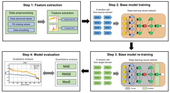Machine learning (ML) methods can mine the hidden degradation information from the aging data [14]. The typical flowchart to develop an ML-based SOH estimation method is shown in Figure 1. Data processing and model training are two critical steps that determine the performance of the SOH estimation [15]. For data preprocessing, the so-called health features (HFs) [16] are extracted from the raw data, which is the foundation and key for ML methods. The extraction methods include direct extraction and indirect extraction methods [17]. The direct extraction method obtains HFs based on the measured raw data directly. For example, the charging time of constant current (CC) and constant voltage (CV) processes [18,19], the slope of the curve during the end of the CC charging process [20], and voltage discrepancy at uniform time intervals [21] were used as HFs in recently published papers. The indirect extraction method obtains HFs based on the reconstructed curves. Commonly used reconstructing methods are incremental capacity (IC) analysis [22], differential voltage (DV) analysis [23], and differential temperature (DT) analysis [16]. For example, multiple peaks can be seen in the IC curve, and each peak reflects the phase transition when the battery is working. With the aging of LiBs, the IC curve shows a specific trend of change, especially the peaks. Therefore, the value, position, width, slope, and area under each peak are often used as HFs. For these kinds of reconstructed curves, filtering methods are required to eliminate the influence of noise. Other indirect HFs include open circuit voltage and ohmic resistance within the ECM or polarization capacitance and resistance derived from electrochemical impedance [24,25]. The main drawback is that additional algorithms are required, increasing its difficulty. Other variables, namely, the sample entropy [26,27] and Kullback–Leibler distance [28], are also used as HFs for SOH estimation.

Based on the pre-processed HFs and SOH values, different ML approaches are employed to train the SOH estimation model, including shallow neural networks, deep learning methods, Gaussian process regression (GPR), support vector machine (SVM), and ensemble learning methods. Although developing the data-driven-based SOH estimation method requires numerous aging data, more and more public aging datasets are available online thanks to the joint efforts of all researchers, which is beneficial for developing advanced health prognostic methods. Some popular public aging datasets are given in

Table 1. Summary of the publicly available battery datasets.

Sources	Refs.
Research & development data repository from Sandia National Labs	[29]
Oxford battery degradation dataset	[30]
Center for Advanced Life Cycle Engineering (CALCE) at the University of Maryland	[31,32]
NASA Ames Prognostic Data Repository (NASA)	[33]
Massachusetts Institute of Technology (MIT) dataset	[34]
The Tongji University dataset	[35]
The Huazhong University of Science and Technology dataset	[36]

.

Currently, the HF-based ML methods for SOH estimation are usually developed based on a single battery dataset, which means that the effectiveness and applicability of the HF extraction strategy cannot be guaranteed toward other battery datasets. For example, Fan et al. [37] used different combinations of HFs to train the SOH estimation model toward the NASA and Oxford aging datasets, respectively. When choosing appropriate HFs, in addition to the principles of easy acquisition, suitability for practical conditions, and a highly relevant degree, the adaptability and universality of different types of batteries are significant. Therefore, it is essential to explore a robust HF extraction strategy that is especially applicable to diverse material types and varied working conditions [38].

On the other hand, when using a single battery dataset to train the SOH estimation model, it usually assumes that the training and testing data have the same distribution. However, such an assumption does not work for different types of batteries or working conditions. Therefore, the well-trained SOH estimation model cannot guarantee an acceptable estimation performance toward other battery datasets. In this case, transfer learning (TL) technology is utilized for such problems [39]. Two strategies, namely, the model parameter fine-tuning and domain adaption methods, are used in recent works for SOH estimation [40].

For the fine-tuning strategy, the data from the source domain is used to train the base model first, and then the specific layer in the base model is re-trained using the data from the target domain while other layers keep frozen. Huang et al. [41] proposed a deep learning model, and the principles of either fine-tuning or rebuilding were applied based on whether the target domain shared the same type of LiBs. However, the HFs used in the source domain and target domain were different according to different source and target domain selections. In another work [42], according to whether the feature expression score (FES) was greater than a threshold, the last fully connected (FC) layer of the base model was fine-tuned or reconstructed. However, the proposed method was only validated inside the same aging datasets (e.g., the NASA aging dataset). In addition, the need for individual fine-tuning for each battery in the target domain significantly increases computational expenses. Zhu et al. [35] randomly selected a battery from the target domain and used its complete cyclic data for TL. They also compared different data selection strategies and concluded that using data from a randomly selected battery can achieve much better results than that from the time-series-based data. In addition, the fine-tuning strategy was applied for the SOH estimation of the battery pack [43].

Domain adaptation methods aim to reduce the disparity in feature distributions between the source and target domains, ultimately enhancing the generalization and accuracy of data-driven models. [44]. Li et al. [45] used transfer component analysis (TCA) to minimize data differences and eliminate redundancy across various datasets. In another work [46], joint distribution adaptation (JDA) was employed to achieve simultaneous adaptation of both the marginal probability and the conditional probability distribution. Fu et al. [38] proposed a feature mapping strategy that first identified the reference cell (RC) and optimal matching cell (OMC) in the source domain and target domain, respectively. Then, a linear matching approach was developed. The cyclic data of the OMC in the target domain was used to re-train the base model. However, for different source and target domains, it is necessary to identify the RC and OMC first, increasing the complexity of the algorithm.

Based on the analysis above, some challenges need to be considered: (1) a universal and effective HF extraction strategy is imperative, especially for different types of batteries and different working conditions; (2) how accurate and robust SOH estimation toward different types of batteries using TL can be ensured. To address these challenges, a universal HF extraction strategy and a deep learning neural network-based transfer learning method are established for SOH estimation in this paper. Three open-source aging datasets, namely the Oxford, CALCE, and NASA aging datasets, are used to validate the effectiveness of the proposed algorithms. The main contributions are as follows:

(1)

To comprehensively reflect the aging characteristics of LiBs and apply them to different battery types and working conditions, a universal HF extraction strategy is proposed. Only partial voltage and current information is required to extract four straightforward and highly relevant HFs.

(2)

To learn the long-term dependency between the HFs and capacity and fulfill TL, a deep learning neural network consisting of the long short-term memory (LSTM) and FC layers is proposed in this paper. For the same battery type (or in the same aging dataset), the proposed neural network is trained using a random-selected battery, and other batteries are used to test the model directly without using the TL strategy.

(3)

To achieve accurate and robust SOH estimation of different types of batteries and different working conditions, the fine-tuning-based TL strategy is used in this paper. The basic principle is to use a random-selected battery in the source domain to train the base model, and then use a random-selected battery in the target domain to re-train the base model, where only the last layer is re-trained and the other layers are frozen.

(4)

Comprehensive verifications are conducted using three popular open-source aging datasets, namely Oxford, CALCE, and NASA aging datasets. Sixteen batteries, featuring two distinct cathode material types, are subjected to cycling under five different operating conditions to assess the efficacy of the proposed methods.

The remainder of the paper is organized as follows: Section 2 introduces the experimental datasets and feature extraction strategy. Section 3 explains the used algorithms. Section 4 gives the results and discussions. Finally, conclusions are summarized in Section 5.

2. Experimental Datasets

Referring to recent research, three open-source aging datasets provided by the University of Oxford [30], the CALCE at the University of Maryland [31,32], and NASA Ames Prognostics Center of Excellence [33] are used in this paper. Note that only the most used data from each dataset is used in this paper, e.g., Cell 1 to 8 from the Oxford aging dataset. Details are explained as follows.

2.1. Oxford Aging Dataset

Eight LiCoO2 (LCO) pouch batteries with 0.74 Ah nominal capacity were selected from the Oxford aging dataset, labeled Cell 1 to Cell 8, respectively. The aging experimental procedures were as follows: (1) The batteries were discharged using a driving cycle obtained from the urban Artemis profile (average current = 1.36 A), and the termination voltage was 2.7 V. (2) Then, the CC charging process was conducted with the batteries with a constant current rate of 2 C until the terminal voltage reached 4.2 V. (3) The above charging–discharging cycle was repeated 100 times, and then a characterization test was conducted to measure the capacity of the batteries. The aging experiment was conducted under 40 °C. The SOH curves of the Oxford aging dataset are shown in Figure 2a. Note that the cycle number in the x-axis represents the number of characterization tests. For example, 45 cycles mean the 45th characterization test after 4500 charging–discharging cycles.

2.2. CALCE Aging Dataset

Four LCO prismatic batteries with 1.14 Ah nominal capacity were selected from the CALCE aging, labeled CS35, CS36, CS37, and CS38, respectively. The aging experimental procedures were as follows: (1) The batteries were discharged using a constant current rate of 1 C, and the termination voltage was 2.7 V. (2) Then, the batteries underwent the same constant current–constant voltage (CC–CV) protocol, where the CC charging current was 0.5 C, and the CV process ended when the current dropped to 0.05 A. (3) The above charging–discharging cycle was repeated until the end-of-experiment criteria were met. The aging experiments were conducted at room temperature (around 25 °C). The SOH curves of the CALCE aging dataset are shown in Figure 2b.

2.3. NASA Aging Dataset

Three 18650 LiNiCoAlO2 (NCA) batteries with 2 Ah nominal capacity were selected from the NASA aging dataset, labeled as B05, B06, and B07, respectively. The aging experimental procedures were as follows: (1) The batteries were discharged with a constant current of 2 A, and the termination voltages were 2.7 V, 2.5 V, and 2.2 V, respectively. (2) The batteries were then fully charged with the CC–CV protocols, where the CC charging current was 1.5 A, and the CV process ended when the current dropped to 0.02 A. (3) The above charging–discharging cycle was repeated until the end-of-experiment criteria were met. The aging experiments were conducted at room temperature (around 24 °C). The SOH curves of the NASA aging dataset are shown in Figure 2c.

According to Figure 2, it is clear that significant differences between the degradation paths of the three aging datasets due to different materials, structures, and working conditions can be observed. In addition, as for the Oxford or CALCE aging datasets, even though the batteries have the same cathode materials and experience the same test protocols, they have different aging paths because of the initial difference. For example, the first charged capacity of the four batteries from CALCE are 1.135 Ah, 1.142 Ah, 1.130 Ah, and 1.137 Ah, respectively, indicating the aging inconsistency. The initial difference could result in more aggressive internal variations as the battery ages. The characteristics of the three aging datasets are given in

Table 2. Characteristics of three open-source aging datasets.

Aging Dataset	Battery Label	Cell Types	Charge C Rate (C)	Charging Cut-Off Voltage (V)	Discharge C Rate (C)	Discharging Cut-Off Voltage (V)	Temperature (°C)	Nominal Capacity (Ah)
Oxford	Cell 1 to Cell 8	LCO	2	4.2	2	2.7	40	0.74
CALCE	CS35 to CS38	LCO	0.5	4.2	1	2.7	25	1.1
NASA	B05	NCA	0.75	4.2	1	2.7	24	2
	B06					2.5
	B07					2.2

.

2.4. Aging Analysis and Feature Extraction

The HF extraction is the foundation and key for building the ML method for SOH estimation. When choosing appropriate HFs, in addition to the principles of easy acquisition, suitability for practical conditions, and high relevant degree, the adaptability and universality toward different types of batteries are significant. Based on this principle, although many valuable HFs are summarized in the Introduction, we want to choose as few neural network inputs as possible but maintain accuracy and robustness simultaneously. Therefore, a universal HF extraction strategy is proposed in this section based on the analysis of three open-source aging datasets.

Note that the CC–CV charging protocol was used in the experiments of the CALCE and NASA, while the CC charging protocol was used in the experiments of Oxford. Hence, only the data from CC charging duration is used to obtain HFs. Figure 3 shows the terminal voltage curves during the CC charging process under different aging states. Taking the Oxford aging dataset as an example, it can be observed that the time for LiBs to reach the upper cut-off voltage (4.2 V) decreases as the battery ages. This phenomenon directly reflects the reduction in usable capacity. Therefore, the charged time during the CC charging process is selected as an HF in many existing research. However, to fulfill the HF-selection principle stated at the beginning of this section, the whole CC charging process cannot be used to obtain the time-related HFs because LiBs are hardly charged from 0% to 100% in practical applications. Hence, the charging duration derived from the specific segment (from 3.8 V to 4.1 V) of the CC charging curves is selected as an HF to represent the battery degradation, denoted as T1. Correspondingly, the charged capacity in this voltage range can be calculated easily since the current remains constant. Therefore, the charged capacity is considered as another HF, denoted as Q1.

The incremental curve analysis (ICA) is a popular method to analyze the aging mechanism of LiBs and is used to extract high-related HFs. The IC curves can be calculated from the CC charging process using a differential equation as follows:

$$\mathrm{I}\mathrm{C}=\frac{dQ}{dV}=I\cdot \frac{dt}{dV}$$

(2)

where Q and V represent the capacity and voltage, respectively, $I$ represents the current, and t is the sampling time.

Figure 4 shows the IC curves under different aging states. We note that the IC curves are further smoothed by the Gaussian filter. Taking the IC curves of the Oxford aging dataset as an example, two peaks can be observed in the middle range of about 3.6–4.1 V. Each peak represents the phase transition process during active material insertion and delamination. With the aging of LiBs, the first peak gradually disappears, and the second peak decreases with a clear trend. In addition, the region beneath the peaks diminishes as the age of the LiBs decreases, indicating a loss of active material and a loss of lithium [47]. As for the other two aging datasets, the IC curves of the CALCE aging dataset also have two peaks and have the same trend as the Oxford aging dataset, while there is only one obvious peak in the IC curves of the NASA aging dataset. To guarantee the universality of the HF extraction strategy, the second peak value and the region beneath the second peak (between 3.8 V and 4.1 V) are selected as HFs, denoted as P1 and A1, respectively.

In many existing research and our previous work [48], temperature information is used to extract valuable HFs. However, to build a uniform feature-extraction strategy considering the commonality of different datasets where the CALCE aging dataset does not provide the temperature information, the temperature information is ignored in this paper. Then, the Pearson correlation coefficient, an efficient method to evaluate the correlation degree between two data sets, is employed in this paper. The expression is as follows:

$$\rho =\frac{\sum _{i=1}^n \left({HF}_i-\overline{HF}\right)\left(C_i-\overline{C}\right)}{\sqrt{\sum _{i=1}^n {\left({HF}_i-\overline{HF}\right)}^2\sum _{i=1}^n {\left(C_i-\overline{C}\right)}^2}}$$

(3)

where ${HF}_i$ and $C_i$ represent HF and SOH, respectively, $\overline{HF}$ and $\overline{C}$ are their mean values, and $n$ is the number of samples. Typically, the Pearson correlation coefficient spans from −1 to 1, with a closer absolute value to 1 indicating a stronger degree of correlation. Figure 5 gives the heat map of the Pearson correlation coefficients of each battery in three open-source aging datasets. It is evident that every Pearson correlation coefficient surpasses 0.95, signifying a robust correlation. In summary, four straightforward and high-related HFs are obtained from the specific segments of the voltage and current curves based on analyzing three aging datasets’ degradation characteristics and commonalities.

3. Related Algorithms

3.1. The Deep Learning Neural Network

Referring to [41,42,46], a deep learning neural network consisting of one LSTM layer, one dropout layer, and three FC layers is established to achieve accurate SOH estimation toward a single aging dataset and fulfill a TL strategy toward different aging datasets. For simplicity, the proposed deep learning neural network is abbreviated as LSTM-FC-NN.

The LSTM layer is used because of its superiority in dealing with time-series data. The LSTM was first created by Hochreiter et al. [49] to solve the information decay during the algorithm back-propagation through time (BPTT). Most gradient-based learning algorithms, such as the Elman neural network [50], suffer either gradient vanishing or gradient explosion when the backflow transfers the information over a long period. To overcome the time dependence problem, the LSTM is proposed with a cell state (memory cell), a hidden state, a forget gate, an input gate, and an output gate, as shown in Figure 6. The expressions are as follows:

$$\begin{gathered} f_t=\mathsf{\sigma }\left(W_f{x}_t+U_f{H}_{t-1}+b_f\right) \\ {i}_t=\mathsf{\sigma }\left(W_i{x}_t+U_i{H}_{t-1}+b_i\right) \\ {o}_t=\mathsf{\sigma }\left(W_o{x}_t+U_o{H}_{t-1}+b_o\right) \\ {c}_t=f_t⨀c_{t-1}+i_t⨀tanh(W_c{x}_t+U_C{H}_{t-1}+b_c) \\ {H}_t=o_t⨀tanh\left(c_t\right) \end{gathered}$$

(4)

where $x_t$ represents the input of the LSTM, $H_t$ represents the hidden state, W and U represent the weight matrices, b represents the bias, $i_t$, $f_t$, $o_t$, and $c_t$ represent the input, forget, output gates, and memory cell, respectively, and $\mathsf{\sigma }$ is the sigmoid activation function. The significant feature of LSTM is the use of different gates to control the information flows. In particular, the input gate determines the new information allowed to pass into the memory cell, while the forget gate identifies the information from the previous memory cell ($c_{t-1}$) that should be disregarded. The output gate is used to calculate the outputs. More details can be found in [51].

Although different batteries have similar declining degradation curves, the specific characteristics are different. As referred to in [52], the FC layers in the base model can serve as the “firewall” to achieve outstanding transfer learning performance. Therefore, three FC layers are used in this paper. In addition, to prevent overfitting, especially when there is limited data, a dropout layer is added to the base model. In the end, the structure of the proposed deep learning neural network is shown in Figure 7. For reproducibility, important hyperparameters are listed in

Table 3. Hyperparameters of the deep learning neural network.

Hyperparameters	Values and Settings
Optimization method	Adam
Number of units in LSTM layer	100
Number of units in FC layers	10/10/1
Dropout rate	0.5
Data split ratio for training base model	80%/10%/10%
Data split ratio for re-training	80%/20%

. Note that all algorithms and computations are executed using MATLAB 2022b.

3.2. Transfer Learning Strategy

Parameter fine-tuning and domain adaptation methods are two commonly used strategies in TL. The parameter fine-tuning method is more straightforward than the domain adaption method. Thus, the fine-tuning-based TL strategy is used in this paper. The principle of the fine-tuning-based TL is shown in Figure 8:

(1)

First, three open-source aging datasets, the Oxford, CALCE, and NASA aging datasets, are represented using different shapes, respectively. Note that different color shades represent the inconsistency between the batteries in the same aging dataset, caused by different initial states, working conditions, and internal variations in material properties from battery manufacturing.

(2)

Second, one of the three aging datasets is selected as the source domain, and the other two are considered the target domains. Then, the cyclic data of a randomly selected battery from the source domain is used to train the base model. And other batteries in the source domain are used to test the base model.

(3)

Third, the fine-tuning-based TL strategy is applied when the target domain is available. The data-selection principle is used to randomly select a battery in the target domain and re-train the base model with its cyclic data using the fine-tuning method. The fine-tuning method in this paper means that only the last FC layer is updated during re-training, while other layers are frozen.

(4)

Finally, other batteries in the target domain are used to test the re-trained model.

By using the random-selected strategy, the accuracy and robustness of the proposed deep learning neural network and fine-tuning-based TL strategy can be thoroughly evaluated.

4. Results and Discussion

This section gives the results of the proposed universal HF extraction strategy and LSTM-FC-NN for SOH estimation on the single aging dataset, as well as the effectiveness of the proposed fine-tuning-based TL strategy toward different types of batteries in detail. Commonly used statistical metrics, namely, the mean absolute error (MAE), root mean square error (RMSE), and the maximum error (MaxE), are used to evaluate the performance quantitively. The MAE gives equal weight to all errors, which can be used to evaluate the accuracy of a regression model. At the same time, the RMSE is more sensitive to outliers and can be used to evaluate the robustness of a model. The MaxE is useful for understanding the magnitude of the largest error. The expressions are as follows:

$$\mathrm{M}\mathrm{A}\mathrm{E}=\frac{1}{N}\sum _{i=1}^N \left|{\widehat{SOH}}_i-{SOH}_i\right|$$

(5)

$$\mathrm{R}\mathrm{M}\mathrm{S}\mathrm{E}=\sqrt{\frac{1}{N}\sum _{i=1}^N {\left({\widehat{SOH}}_i-{SOH}_i\right)}^2}$$

(6)

$$\mathrm{M}\mathrm{a}\mathrm{x}\mathrm{E}=max\left|{\widehat{SOH}}_i-{SOH}_i\right|$$

(7)

where ${\widehat{SOH}}_i$ represents the predicted value, ${SOH}_i$ represents the reference value, and $N$ is the number of samples.

4.1. Results of the Single Aging Dataset

This section separately evaluates the proposed deep learning neural network for SOH estimation using three open-source aging datasets. It first verifies the effectiveness of the proposed universal HFs extraction strategy and proves that the proposed LSTM-FC-NN model can achieve accurate and robust SOH estimation toward different battery types. Note that the training and evaluation principle for the same type of batteries is that a random-selected battery is used to train the base model, and other batteries are used to test the base model directly without using the TL strategy.

4.1.1. Oxford Aging Dataset

Table 4. Estimation results of the Oxford aging dataset.

Train	Test	MAE (%)	RMSE (%)	MaxE (%)
Cell 1	Cell 2	0.22	0.28	0.59
	Cell 3	0.21	0.27	0.52
	Cell 4	0.29	0.36	0.89
	Cell 5	0.49	0.56	1.05
	Cell 6	0.56	0.61	1.02
	Cell 7	0.45	0.53	1.07
	Cell 8	0.56	0.62	1.09

gives the statistical metrics of the case that Cell 1 in the Oxford aging dataset is randomly selected to train the base model, and other batteries are used to test the base model directly without using the TL strategy.

Table 5. Estimation results of all cases in the Oxford aging dataset.

Unit: %	Cell 1	Cell 2	Cell 3	Cell 4	Cell 5	Cell 6	Cell 7	Cell 8
MAE *	0.37	0.39	0.32	0.34	0.32	0.34	0.29	0.32
RMSE *	0.43	0.48	0.40	0.42	0.39	0.39	0.35	0.37
MaxE *	0.84	0.95	0.83	0.86	0.82	0.75	0.71	0.70

* The MAE, RMSE, and MaxE are the mean values.

gives the results where another battery is randomly selected to train the model, e.g., Cell 2 to Cell 7, and the MAE, RMSE, and MaxE in Table 5 are the mean values. For example, the second column in Table 5 represents that Cell 2 is used to train the base model, and the other seven cells are used to test the base model. Then, the MAE, RMSE, and MaxE are the mean values of the seven testing results. Correspondingly, the eight curves in Figure 9 represent which battery is used to train the base model.

Overall, it can be seen from Figure 9 that no matter which battery is randomly selected to train the base model, the base model can achieve accurate SOH estimation results toward other batteries without using the TL strategy. Specifically, as an example, Figure 9a gives the results where Cell 2 to Cell 7 are used to train the base model in turn, and Cell 1 is used to test the base model. It can be observed that all seven estimated SOH curves can follow the actual SOH curves quite well. The MaxE is merely 1.09% when Cell 8 is used to train the base model, according to Table 4. In addition, the mean values of MAE and RMSE are only 0.37% and 0.43%, respectively, according to Table 5. As for other evaluation cases in Table 5, the estimation results demonstrate that the proposed universal HF strategy and LSTM-FC-NN model can achieve accurate and robust SOH estimation toward the Oxford aging dataset.

4.1.2. CALCE Aging Dataset

Table 6. Estimation results of the CALCE aging dataset.

Train	Test	MAE (%)	RMSE (%)	MaxE (%)
CS35	CS36	0.51	0.70	2.55
	CS37	0.48	0.59	3.06
	CS38	0.63	0.75	3.32
CS36	CS35	0.51	0.61	2.54
	CS37	0.57	0.70	3.38
	CS38	0.80	0.94	3.70
CS37	CS35	0.63	0.94	3.87
	CS36	0.74	1.04	5.08
	CS38	0.48	0.60	3.04
CS38	CS35	1.11	1.87	8.30
	CS36	1.21	1.83	9.71
	CS37	0.66	0.90	3.60
Mean values	-	0.69	0.96	4.35

gives the results that a random-selected battery from the CALCE aging dataset is used to train the base model, and other batteries are used to test the base model without using the TL strategy. Correspondingly, Figure 10 illustrates the estimation results.

Similar to the Oxford aging dataset results, on which a battery is used to train the base model, the model can achieve accurate and robust SOH estimation toward other batteries without the TL strategy. For example, Figure 10d shows the estimation results of CS38 using different battery-based base models. It can be observed that no matter which battery is used to train the base model, the base model can obtain accurate estimation results toward CS38. The estimated SOH curves can always follow the actual aging path, even in some slight range fluctuation. In addition, the estimation errors rarely exceed absolute 2%, demonstrating the proposed method’s robustness. However, for CS35 and CS36, when evaluated using the CS38-based base model, the results are slightly worse than other battery-based models. This is because the aging path of CS38 is quite different from that of CS35 and CS36, especially when the SOH drops below 80%, as shown in Figure 2b. When the SOH drops below 80%, the internal electrochemical reaction becomes more uncontrollable, resulting in quicker and more different aging paths. Therefore, significant estimation errors and MaxE occur when the SOH drops below 80%. At the same time, there is consistency between the estimated and actual SOH curves when the SOH is higher than 80%, as shown in Figure 10a,b. Overall, the last row in Table 6 represents the mean values of the corresponding columns. It can be concluded that the mean values of MAE and RMSE are 0.69% and 0.96%, respectively, demonstrating the accuracy and robustness of the proposed model toward the CALCE aging dataset.

4.1.3. NASA Aging Dataset

Table 7. Estimation results of the NASA aging dataset.

Train	Test	MAE (%)	RMSE (%)	MaxE (%)
B05	B06	3.40	3.88	12.43
	B06_retrain	1.39	1.86	8.21
	B07	0.63	0.97	5.68
B06	B05	2.94	3.12	4.85
	B07	1.99	2.22	5.00
B07	B05	0.72	0.95	5.10
	B06	3.40	3.91	12.72
	B06_retrain	1.37	1.93	8.66

gives the results that a random-selected battery from the NASA aging dataset is used to train the base model, and other batteries are used to test the model directly without using the TL strategy. Figure 11 compares the estimated SOH curves based on different base models and actual SOH curves and the estimated errors.

According to Table 7, it can be concluded that when the B05 is used to train the base model, the base model can achieve accurate SOH estimation toward B07 but not B06. The MAE and RMSE of B07 are 0.63% and 0.97%, respectively, while the MAE and RMSE of B06 are 3.40% and 3.88%, respectively. As shown in Figure 11c, the estimated SOH curve based on B05 can follow the actual aging path quite well, but in Figure 11b, there is a significant difference between the estimated SOH curve based on B05 and the actual SOH curve. The same results can be observed when B07 is used to train the base model. As for the case when B06 is used to train the base model, it can be seen from Figure 11a,c that the estimated curves based on B06 cannot follow the real SOH curves well, e.g., the blue line in Figure 11a and the yellow line in Figure 11c. The reasons can be explained as follows. First, the initial SOH of these three batteries is quite different, indicating 0.92%, 1.01%, and 0.94% for B05, B06, and B07, respectively, as shown in Figure 2c. Second, the discharging protocols for these three batteries are different, as summarized in Table 2. Different discharging cut-off voltages would result in different depths of discharge, which is essential for battery aging. The initial differences are bound to result in inconsistencies in the aging paths of different batteries, and different cycling protocols exacerbate the inconsistencies. Therefore, as shown in Figure 2, it can be observed that the differences between different aging paths of the NASA aging dataset are more evident than the other two aging datasets.

Since the aging path of B06 is quite different from B05 and B07, the fine-tuning-based TL strategy is used to improve the accuracy. Figure 12 compares the estimation results of B06 with or without using the fine-tuning-based TL strategy, and the corresponding results are given in Table 7. After fine-tuning the base model, the re-trained model can perform much better. The estimated SOH curves can follow the actual SOH curve well. The MAE and RMSE after using the TL strategy are 1.39% and 1.86%, respectively, decreasing by 59% and 52%, respectively. In summary, the effectiveness of the proposed LSTM-FC-NN model and fine-tuning-based TF strategy is verified toward the NASA aging dataset.

In summary, three open-source aging datasets are used separately to evaluate the effectiveness of the proposed universal HF extraction strategy and LSTM-FC-NN model for SOH estimation in this section. On the one hand, from the results of the Oxford and CALCE aging datasets, it can be concluded that when the training and testing batteries are the same battery type and have the same aging protocol, the estimations are accurate and reliable, whatever the training dataset. On the other hand, from the results of the NASA aging dataset, it can be concluded that when the testing battery has a significantly different aging path from the training one, the estimations cannot be guaranteed. In this case, the fine-tuning-based TL strategy can be used to improve the adaptivity of the trained model toward the testing battery, which builds the foundation for the following results.

4.2. Results of the Proposed Transfer Learning Strategy between Different Aging Datasets

This section gives the results of the proposed fine-tuning-based TL strategy between three open-source aging datasets in detail. As shown in Figure 8, the evaluation principle is that one of the three aging datasets is randomly selected as the source domain, and the other two aging datasets are then used separately as the target domain. Then, a randomly selected battery from the source domain is used to train the base model. Next, one of the batteries in the target domain is selected randomly, and its cyclic data is used to fine-tune the base model. Finally, the re-trained model is tested using other batteries in the target domain. The following three subsections explain the results in detail.

4.2.1. Transfer Learning between Oxford and CALCE Aging Datasets

Figure 13 gives the results that Cell 1 is used to train the base model, CS38 is randomly selected to re-train the base model using the fine-tuning strategy, and other batteries in the CALCE aging datasets are used to test the re-trained model. Note that the blue lines (labeled as Before TL) give the estimated SOH curves using the base model directly, and the yellow lines (labeled as After TL) give the estimated SOH curves using the fine-tuned base model.

It can be observed that although the overall trend of the estimated SOH curves without using the TL strategy has the same downtrend as the actual SOH curves, there are significant estimation errors between them. That is because the LSTM layer can learn the long-term dependency between the input features and SOH, but the last FC layer determines the final output. Therefore, the re-trained model can adapt to the target domain when the last FC layer is updated. Then, the estimated SOH curves can track the real SOH curves quite well, even with slight fluctuation. Specifically, according to

Table 8. The results of the TL strategy from Oxford to CALCE.

Source/Target	Test	Method	MAE (%)	RMSE (%)	MaxE (%)
Cell 1/CS38	CS35	Before TL	10.61	11.40	19.88
		After TL	0.68	0.95	3.49
	CS36	Before TL	10.96	12.12	20.45
		After TL	0.74	1.08	4.71
	CS37	Before TL	10.68	11.26	19.68
		After TL	0.59	0.72	3.06

, the MAE and RMSE of CS35 after using the TL strategy are 0.68% and 0.95%, respectively, which is even better than the results in Table 6.

Figure 14 illustrates that CS35 is used to train the base model, and Cell 4 is used to fine-tune the base model. The corresponding results are summarized in

Table 9. The results of the TL strategy from CALCE to Oxford.

Source/Target	Test	Method	MAE (%)	RMSE (%)	MaxE (%)
CS35/Cell 4	Cell 1	Before TL	8.11	8.19	9.31
		After TL	0.35	0.42	0.90
	Cell 2	Before TL	8.26	8.32	9.21
		After TL	0.26	0.32	0.64
	Cell 3	Before TL	8.15	8.22	9.27
		After TL	0.32	0.36	0.67
	Cell 5	Before TL	8.63	8.69	9.52
		After TL	0.46	0.57	1.11

. Similar results can be observed in Figure 14 that the estimated SOH curves based on the base model have the same downtrend as the actual SOH curves, but there are significant errors between them. After fine-tuning the base model, the estimated SOH curves can track the actual SOH curves quite well. The MAE and RMSE are limited to 0.46% and 0.57%, respectively. Overall, the above results between the Oxford and CALCE aging datasets demonstrate the validity of the proposed LSTM-FC-NN model and the fine-tuning-based TL strategy.

4.2.2. Transfer Learning between CALCE and NASA Aging Datasets

The mutual estimation results of the TL strategy between the CALCE and NASA aging datasets are given in Figure 15 and Figure 16, respectively. As an example, Figure 15 shows the estimation results of CS36, CS37, and CS38 with or without using TL. The corresponding results are summarized in

Table 10. The results of the TL strategy from NASA to CALCE.

Source/Target	Evaluation	Method	MAE (%)	RMSE (%)	MaxE (%)
B05/CS35	CS36	Before TL	5.66	6.45	13.42
		After TL	0.58	0.85	3.15
	CS37	Before TL	4.26	4.99	12.59
		After TL	0.63	0.78	3.16
	CS38	Before TL	4.20	5.04	12.83
		After TL	0.80	0.95	3.40

. The overall trend of the estimated curves before using the TL strategy is similar to the real ones, but significant gaps can be found. After updating the last FC layer of the base model, the re-trained model can track the descent SOH curves well. Furthermore, the proposed LSTM-FC-NN model showcases robustness, with the MAE and RMSE constrained to 0.80% and 0.95%, respectively.

Figure 16 gives the estimation results of B05 and B06 with or without using TL, and the corresponding results are summarized in

Table 11. The results of the TL strategy from CALCE to NASA.

Source/Target	Test	Method	MAE (%)	RMSE (%)	MaxE (%)
CS35/B07	B05	Before TL	19.91	20.97	28.29
		After TL	0.70	0.95	5.12
	B06	Before TL	10.77	14.42	27.38
		After TL	3.36	3.83	12.48

. As analyzed in Section 4.1.3, the model trained using data of B07 can achieve accurate estimation toward B05 but not B06. Similar results can be found in this TL case. As shown in Figure 16a, the B07-based model can achieve accurate estimation toward B05 after implementing the TL strategy. As for B06, the B07-based model improves the estimation accuracy after implementing the TL strategy, and the MAE and RMSE decreased by 68.80% and 73.43%, respectively.

4.2.3. Transfer Learning between NASA and Oxford Aging Datasets

The mutual estimation results of the TL strategy between the NASA and Oxford aging datasets are shown in Figure 17 and Figure 18, respectively. The same estimation results can be found that although the estimated SOH curves before using the TL strategy can follow the overall trend with the real SOH curves, there are significant gaps between them. After fine-tuning the base model, the estimated SOH curves can accurately track the real ones. The results corresponding to Figure 17 and Figure 18 are given in

Table 12. The results of the TL strategy from NASA to Oxford.

Source/Target	Test	Method	MAE (%)	RMSE (%)	MaxE (%)
B05/Cell 2	Cell 1	Before TL	19.22	19.59	26.06
		After TL	0.25	0.29	0.52
	Cell 3	Before TL	19.34	19.70	25.86
		After TL	0.17	0.20	0.38
	Cell 4	Before TL	19.26	19.60	25.41
		After TL	0.32	0.36	0.65
	Cell 5	Before TL	20.04	20.31	25.99
		After TL	0.40	0.47	0.87

and

Table 13. The results of the TL strategy from Oxford to NASA.

Source/Target	Test	Method	MAE (%)	RMSE (%)	MaxE (%)
Cell 6/B05	B06	Before TL	4.96	6.03	13.38
		After TL	2.00	2.53	10.19
	B07	Before TL	10.66	11.26	15.94
		After TL	0.87	1.12	4.84

, respectively. For the TL strategy from NASA to Oxford, the MAE, RMSE, and MaxE are limited to 0.4%, 0.47%, and 0.87%, respectively, demonstrating the effectiveness of the proposed deep learning neural network and fine-tuning-based TL strategy.

In summary, this section evaluates the effectiveness of the proposed LSTM-FC-NN model and fine-tuning-based TL strategy using three open-source aging datasets. It can be concluded that although the estimated curves based on the base model can follow the overall downtrend of the actual curves, there are significant gaps between them. This result is because the LSTM layer can learn the long-term dependency between the inputs and outputs, and the overall degradation trend of different types of batteries is similar. However, the final outputs are determined by the last layer of the base model. Therefore, after using the fine-tuning strategy to update the last FC layer of the model, the re-trained model can adapt to the target domain quite well and achieve accurate and robust estimation results.

Table 14. The comparison of results with or without the TL strategy.

Unit: (%)		Oxford		CALCE		NASA
		MAE *	RMSE *	MAE *	RMSE *	MAE *	RMSE *
Oxford	Before TL	-		12.78	13.55	7.81	8.65
	After TL			0.93	1.18	1.09	1.41
CALCE	Before TL	8.88	8.97	-		15.34	17.70
	After TL	0.42	0.51			0.92	1.24
NASA	Before TL	19.83	20.13	6.55	7.37	-
	After TL	0.41	0.48	0.86	1.09

* The MAE and RMSE are the mean values of all evaluation cases.

compares the results with or without using the TL strategy between three aging datasets. The first column represents the source domain, and the first row represents the target domain. The MAEs and RMSEs in Table 14 are the mean values of all evaluation cases from the source domain to the target domain. It can be concluded that with the fine-tuning-based TL strategy, the accuracy of SOH estimation improves significantly, and the MAE and RMSE are limited to 1.09% and 1.41%, respectively. In addition to the model accuracy, the number of learnable parameters and training time are used to analyze the algorithm complexity with or without the TL. According to the hyperparameter setting, the proposed deep learning neural network has 43,100 learnable parameters. If the whole model needs to be re-trained toward the target domain, 43,100 learnable parameters must be involved in the training process. However, only the last FC layer is updated for the fine-tuning-based TL method, meaning only 11 learnable parameters are involved. As for the training time, take training B05 as an example. When training the entire model, it took 14.43 s, and when re-training the model using the fine-tuning method, it took only 7.08 s. Note that this is the average time when training 10 times.

4.3. Future Work

This work comprehensively verifies the effectiveness of the proposed LSTM-FC-NN model using a universal HF extraction strategy and the fine-tuning-based TL strategy for SOH estimation using three open-source aging datasets with different material types and working conditions. However, there are some limitations beyond this research. First, this research does not consider the LiFePO₄ (LFP) cell, which is a commonly used type of LiB. Second, the batteries used in this research were cycled under CC–CV charge–CC discharge protocols, which are different from real-world working conditions. Third, the results of the NASA aging dataset are worse than the other two because of severe inconsistency and capacity regeneration. In our forthcoming research, we plan to investigate a broader range of battery types, including those cycled under dynamic operational conditions. The accuracy and robustness of the proposed method will be improved according to the specific characteristics of different types of batteries.

5. Conclusions

A universal HF extraction strategy and an LSTM-FC-NN model are proposed in this paper for accurate and robust SOH estimation. In addition, the fine-tuning-based TL strategy is developed considering the difference in data distribution between different types of batteries. Sixteen batteries, featuring two distinct cathode material types, are subjected to cycling under five different operating conditions to assess the efficacy of the proposed methods. The main conclusions are summarized as follows:

(1)

Four straightforward HFs, including charged time, charged capacity, peak value of the IC curve, and area under the IC peak, were extracted from partial voltage curves to reflect the battery degradation of different battery types. The Pearson correlation analysis demonstrates that the four extracted HFs are highly related to battery capacity.

(2)

A deep learning neural network consisting of one LSTM layer, one dropout layer, and three FC layers was proposed to estimate the SOH accurately. The effectiveness of the proposed LSTM-FC-NN model with the HFs was verified using three open-source aging datasets. The MAE and RMSE are less than 1.21% and 1.83%, respectively.

(3)

The fine-tuning method was used to transfer learning between three aging datasets where a random-selected battery from the target domain was utilized to re-train the base model. The mutual evaluation between the three aging datasets demonstrates the validity of the TL strategy, with the MAE and RMSE limited to 1.09% and 1.41%, respectively.

References

1. Dai, H.; Jiang, B.; Hu, X.; Lin, X.; Wei, X.; Pecht, M. Advanced Battery Management Strategies for a Sustainable Energy Future: Multilayer Design Concepts and Research Trends. Renew. Sustain. Energy Rev. 2021, 138, 110480. [Google Scholar] [CrossRef]
2. Ge, M.F.; Liu, Y.; Jiang, X.; Liu, J. A Review on State of Health Estimations and Remaining Useful Life Prognostics of Lithium-Ion Batteries. Meas. J. Int. Meas. Confed. 2021, 174, 109057. [Google Scholar] [CrossRef]
3. Liu, S.; Nie, Y.; Tang, A.; Li, J.; Yu, Q.; Wang, C. Online Health Prognosis for Lithium-Ion Batteries under Dynamic Discharge Conditions over Wide Temperature Range. eTransportation 2023, 18, 100296. [Google Scholar] [CrossRef]
4. Xiong, R.; Li, L.; Tian, J. Towards a Smarter Battery Management System: A Critical Review on Battery State of Health Monitoring Methods. J. Power Sources 2018, 405, 18–29. [Google Scholar] [CrossRef]
5. Gao, Y.; Liu, K.; Zhu, C.; Zhang, X.; Zhang, D. Co-Estimation of State-of-Charge and State-of- Health for Lithium-Ion Batteries Using an Enhanced Electrochemical Model. IEEE Trans. Ind. Electron. 2022, 69, 2684–2696. [Google Scholar] [CrossRef]
6. Chen, L.; Lü, Z.; Lin, W.; Li, J.; Pan, H. A New State-of-Health Estimation Method for Lithium-Ion Batteries through the Intrinsic Relationship between Ohmic Internal Resistance and Capacity. Measurement 2018, 116, 586–595. [Google Scholar] [CrossRef]
7. Du, C.Q.; Shao, J.B.; Wu, D.M.; Ren, Z.; Wu, Z.Y.; Ren, W.Q. Research on Co-Estimation Algorithm of SOC and SOH for Lithium-Ion Batteries in Electric Vehicles. Electronics 2022, 11, 181. [Google Scholar] [CrossRef]
8. Schwunk, S.; Armbruster, N.; Straub, S.; Kehl, J.; Vetter, M. Particle Filter for State of Charge and State of Health Estimation for Lithium-Iron Phosphate Batteries. J. Power Sources 2013, 239, 705–710. [Google Scholar] [CrossRef]
9. Niri, M.F.; Liu, K.; Apachitei, G.; Román-Ramírez, L.A.; Lain, M.; Widanage, D.; Marco, J. Quantifying Key Factors for Optimised Manufacturing of Li-Ion Battery Anode and Cathode via Artificial Intelligence. Energy AI 2022, 7, 100129. [Google Scholar] [CrossRef]
10. Cui, X.; Garg, A.; Trang Thao, N.; Trung, N.T. Machine Learning Approach for Solving Inconsistency Problems of Li-Ion Batteries during the Manufacturing Stage. Int. J. Energy Res. 2020, 44, 9194–9204. [Google Scholar] [CrossRef]
11. Mao, J.; Miao, J.; Lu, Y.; Tong, Z. Machine Learning of Materials Design and State Prediction for Lithium Ion Batteries. Chin. J. Chem. Eng. 2021, 37, 1–11. [Google Scholar] [CrossRef]
12. Wei, Z.; Yang, X.; Li, Y.; He, H.; Li, W.; Sauer, D.U. Machine Learning-Based Fast Charging of Lithium-Ion Battery by Perceiving and Regulating Internal Microscopic States. Energy Storage Mater. 2023, 56, 62–75. [Google Scholar] [CrossRef]
13. Jiang, B.; Berliner, M.D.; Lai, K.; Asinger, P.A.; Zhao, H.; Herring, P.K.; Bazant, M.Z.; Braatz, R.D. Fast Charging Design for Lithium-Ion Batteries via Bayesian Optimization. Appl. Energy 2022, 307, 118244. [Google Scholar] [CrossRef]
14. Ng, M.-F.; Zhao, J.; Yan, Q.; Conduit, G.J.; Seh, Z.W. Predicting the State of Charge and Health of Batteries Using Data-Driven Machine Learning. Nat. Mach. Intell. 2020, 2, 161–170. [Google Scholar] [CrossRef]
15. Ren, Z.; Du, C. A Review of Machine Learning State-of-Charge and State-of-Health Estimation Algorithms for Lithium-Ion Batteries. Energy Rep. 2023, 9, 2993–3021. [Google Scholar] [CrossRef]
16. Lin, M.; Wu, D.; Meng, J.; Wu, J.; Wu, H. A Multi-Feature-Based Multi-Model Fusion Method for State of Health Estimation of Lithium-Ion Batteries. J. Power Sources 2022, 518, 230774. [Google Scholar] [CrossRef]
17. Hu, X.; Che, Y.; Lin, X.; Onori, S. Battery Health Prediction Using Fusion-Based Feature Selection and Machine Learning. IEEE Trans. Transp. Electrif. 2021, 7, 382–398. [Google Scholar] [CrossRef]
18. Cao, M.; Zhang, T.; Wang, J.; Liu, Y. A Deep Belief Network Approach to Remaining Capacity Estimation for Lithium-Ion Batteries Based on Charging Process Features. J. Energy Storage 2022, 48, 103825. [Google Scholar] [CrossRef]
19. Deng, Y.; Ying, H.; Jiaqiang, E.; Zhu, H.; Wei, K.; Chen, J.; Zhang, F.; Liao, G. Feature Parameter Extraction and Intelligent Estimation of the State-of-Health of Lithium-Ion Batteries. Energy 2019, 176, 91–102. [Google Scholar] [CrossRef]
20. Yang, D.; Zhang, X.; Pan, R.; Wang, Y.; Chen, Z. A Novel Gaussian Process Regression Model for State-of-Health Estimation of Lithium-Ion Battery Using Charging Curve. J. Power Sources 2018, 384, 387–395. [Google Scholar] [CrossRef]
21. Goh, H.H.; Lan, Z.; Zhang, D.; Dai, W.; Kurniawan, T.A.; Goh, K.C. Estimation of the State of Health (SOH) of Batteries Using Discrete Curvature Feature Extraction. J. Energy Storage 2022, 50, 104646. [Google Scholar] [CrossRef]
22. Zhang, Y.; Liu, Y.; Wang, J.; Zhang, T. State-of-Health Estimation for Lithium-Ion Batteries by Combining Model-Based Incremental Capacity Analysis with Support Vector Regression. Energy 2022, 239, 121986. [Google Scholar] [CrossRef]
23. Mohtat, P.; Lee, S.; Siegel, J.B.; Stefanopoulou, A.G. Comparison of Expansion and Voltage Differential Indicators for Battery Capacity Fade. J. Power Sources 2022, 518, 230714. [Google Scholar] [CrossRef]
24. Lyu, Z.; Wang, G.; Tan, C. A Novel Bayesian Multivariate Linear Regression Model for Online State-of-Health Estimation of Lithium-Ion Battery Using Multiple Health Indicators. Microelectron. Reliab. 2022, 131, 114500. [Google Scholar] [CrossRef]
25. Yang, D.; Wang, Y.; Pan, R.; Chen, R.; Chen, Z. State-of-Health Estimation for the Lithium-Ion Battery Based on Support Vector Regression. Appl. Energy 2018, 227, 273–283. [Google Scholar] [CrossRef]
26. Cao, M.; Zhang, T.; Yu, B.; Liu, Y. A Method for Interval Prediction of Satellite Battery State of Health Based on Sample Entropy. IEEE Access 2019, 7, 141549–141561. [Google Scholar] [CrossRef]
27. Hu, X.; Jiang, J.; Cao, D.; Egardt, B. Battery Health Prognosis for Electric Vehicles Using Sample Entropy and Sparse Bayesian Predictive Modeling. IEEE Trans. Ind. Electron. 2016, 63, 2645–2656. [Google Scholar] [CrossRef]
28. Lin, M.; Zeng, X.; Wu, J. State of Health Estimation of Lithium-Ion Battery Based on an Adaptive Tunable Hybrid Radial Basis Function Network. J. Power Sources 2021, 504, 230063. [Google Scholar] [CrossRef]
29. Doughty, D.H.; Roth, E.P.; Nagasubramanian, G.; Ong, M.D.; Robinson, D.B.; Arslan, I.; Situ, A.-I.; Sullivan, J.P.; Subramanian, A.; Huang, J. Degradation of Commercial Lithium-Ion Cells as a Function of Chemistry and Cycling Conditions. J. Electrochem. Soc. 2020, 167, 120532. [Google Scholar] [CrossRef]
30. Christoph, R.B. Diagnosis and Prognosis of Degradation in Lithium-Ion Batteries. Ph.D. Thesis, Department of Engineering Science, University of Oxford, Oxford, UK, 2017. [Google Scholar]
31. Xing, Y.; Ma, E.W.M.; Tsui, K.L.; Pecht, M. An Ensemble Model for Predicting the Remaining Useful Performance of Lithium-Ion Batteries. Microelectron. Reliab. 2013, 53, 811–820. [Google Scholar] [CrossRef]
32. He, W.; Williard, N.; Osterman, M.; Pecht, M. Prognostics of Lithium-Ion Batteries Based on Dempster–Shafer Theory and the Bayesian Monte Carlo Method. J. Power Sources 2011, 196, 10314–10321. [Google Scholar] [CrossRef]
33. Lau, S. Intelligent Systems Division. Available online: https://ti.arc.nasa.gov/project/prognostic-data-repository/ (accessed on 21 September 2021).
34. Severson, K.A.; Attia, P.M.; Jin, N.; Perkins, N.; Jiang, B.; Yang, Z.; Chen, M.H.; Aykol, M.; Herring, P.K.; Fraggedakis, D.; et al. Data-Driven Prediction of Battery Cycle Life before Capacity Degradation. Nat. Energy 2019, 4, 383–391. [Google Scholar] [CrossRef]
35. Zhu, J.; Wang, Y.; Huang, Y.; Bhushan Gopaluni, R.; Cao, Y.; Heere, M.; Mühlbauer, M.J.; Mereacre, L.; Dai, H.; Liu, X.; et al. Data-Driven Capacity Estimation of Commercial Lithium-Ion Batteries from Voltage Relaxation. Nat. Commun. 2022, 13, 2261. [Google Scholar] [CrossRef] [PubMed]
36. Ma, G.; Xu, S.; Jiang, B.; Cheng, C.; Yang, X.; Shen, Y.; Yang, T.; Huang, Y.; Ding, H.; Yuan, Y. Real-Time Personalized Health Status Prediction of Lithium-Ion Batteries Using Deep Transfer Learning. Energy Environ. Sci. 2022, 15, 4083–4094. [Google Scholar] [CrossRef]
37. Fan, L.; Wang, P.; Cheng, Z. A Remaining Capacity Estimation Approach of Lithium-Ion Batteries Based on Partial Charging Curve and Health Feature Fusion. J. Energy Storage 2021, 43, 103115. [Google Scholar] [CrossRef]
38. Fu, S.; Tao, S.; Fan, H.; He, K.; Liu, X.; Tao, Y.; Zuo, J.; Zhang, X.; Wang, Y.; Sun, Y. Data-Driven Capacity Estimation for Lithium-Ion Batteries with Feature Matching Based Transfer Learning Method. Appl. Energy 2024, 353, 121991. [Google Scholar] [CrossRef]
39. Yang, Y.; Zhao, L.; Yu, Q.; Liu, S.; Zhou, G.; Shen, W. State of Charge Estimation for Lithium-Ion Batteries Based on Cross-Domain Transfer Learning with Feedback Mechanism. J. Energy Storage 2023, 70, 108037. [Google Scholar] [CrossRef]
40. Liu, K.; Peng, Q.; Che, Y.; Zheng, Y.; Li, K.; Teodorescu, R.; Widanage, D.; Barai, A. Transfer Learning for Battery Smarter State Estimation and Ageing Prognostics: Recent Progress, Challenges, and Prospects. Adv. Appl. Energy 2023, 9, 100117. [Google Scholar] [CrossRef]
41. Huang, K.; Yao, K.; Guo, Y.; Lv, Z. State of Health Estimation of Lithium-Ion Batteries Based on Fine-Tuning or Rebuilding Transfer Learning Strategies Combined with New Features Mining. Energy 2023, 282, 128739. [Google Scholar] [CrossRef]
42. Tan, Y.; Tan, Y.; Zhao, G.; Zhao, G. Transfer Learning with Long Short-Term Memory Network for State-of-Health Prediction of Lithium-Ion Batteries. IEEE Trans. Ind. Electron. 2020, 67, 8723–8731. [Google Scholar] [CrossRef]
43. Shu, X.; Shen, J.; Li, G.; Zhang, Y.; Chen, Z.; Liu, Y. A Flexible State-of-Health Prediction Scheme for Lithium-Ion Battery Packs with Long Short-Term Memory Network and Transfer Learning. IEEE Trans. Transp. Electrif. 2021, 7, 2238–2248. [Google Scholar] [CrossRef]
44. Pan, S.J.; Yang, Q. A Survey on Transfer Learning. IEEE Trans. Knowl. Data Eng. 2010, 22, 1345–1359. [Google Scholar] [CrossRef]
45. Li, Y.; Sheng, H.; Cheng, Y.; Stroe, D.I.; Teodorescu, R. State-of-Health Estimation of Lithium-Ion Batteries Based on Semi-Supervised Transfer Component Analysis. Appl. Energy 2020, 277, 115504. [Google Scholar] [CrossRef]
46. Ma, Y.; Shan, C.; Gao, J.; Chen, H. Multiple Health Indicators Fusion-Based Health Prognostic for Lithium-Ion Battery Using Transfer Learning and Hybrid Deep Learning Method. Reliab. Eng. Syst. Saf. 2023, 229, 108818. [Google Scholar] [CrossRef]
47. Pastor-Fernández, C.; Yu, T.F.; Widanage, W.D.; Marco, J. Critical Review of Non-Invasive Diagnosis Techniques for Quantification of Degradation Modes in Lithium-Ion Batteries. Renew. Sustain. Energy Rev. 2019, 109, 138–159. [Google Scholar] [CrossRef]
48. Ren, Z.; Du, C.; Ren, W. State of Health Estimation of Lithium-Ion Batteries Using a Multi-Feature-Extraction Strategy and PSO-NARXNN. Batteries 2023, 9, 7. [Google Scholar] [CrossRef]
49. Kolen, J.F.; Kremer, S.C. Gradient Flow in Recurrent Nets: The Difficulty of Learning LongTerm Dependencies. In A Field Guide to Dynamical Recurrent Networks; Wiley-IEEE Press: New York, NY, USA, 2010; pp. 237–243. [Google Scholar] [CrossRef]
50. Li, X.; Wang, Z.; Zhang, L. Co-Estimation of Capacity and State-of-Charge for Lithium-Ion Batteries in Electric Vehicles. Energy 2019, 174, 33–44. [Google Scholar] [CrossRef]
51. Understanding LSTM Networks—Colah’s Blog. Available online: http://colah.github.io/posts/2015-08-Understanding-LSTMs/ (accessed on 11 October 2021).
52. Zhang, C.L.; Luo, J.H.; Wei, X.S.; Wu, J. In Defense of Fully Connected Layers in Visual Representation Transfer. In Pacific Rim Conference on Multimedia; Springer International Publishing: Cham, Switzerland, 2018; Volume 10736, pp. 807–817. [Google Scholar] [CrossRef]
Figure 1. The procedures to build an ML-based SOH estimation method.
Batteries 09 00585 g001
Figure 2. Degradation paths of three aging datasets: (a) Oxford dataset, (b) CALCE dataset, and (c) NASA dataset.
Batteries 09 00585 g002
Figure 3. The terminal voltage curves under different aging states: (a) Oxford dataset, (b) CALCE dataset, and (c) NASA dataset. (EOL means end of life).
Batteries 09 00585 g003
Figure 4. The IC curves under different aging states: (a) Oxford dataset, (b) CALCE dataset, and (c) NASA dataset.
Batteries 09 00585 g004
Figure 5. Heat map of the Pearson correlation coefficient of each battery.
Batteries 09 00585 g005
Figure 6. The structure of LSTM.
Batteries 09 00585 g006
Figure 7. The structure of the proposed deep learning neural network.
Batteries 09 00585 g007
Figure 8. The principle of the fine-tuning-based TL strategy.
Batteries 09 00585 g008
Figure 9. Estimation results of the Oxford aging dataset: (a) Cell 1; (b) Cell 2; (c) Cell 3; (d) Cell 4.
Batteries 09 00585 g009
Figure 10. Estimation results of the CALCE aging dataset: (a) CS35; (b) CS36; (c) CS37; (d) CS38.
Batteries 09 00585 g010
Figure 11. Estimation results of the NASA aging dataset: (a) B05; (b) B06; (c) B07.
Batteries 09 00585 g011
Figure 12. Estimation results of B06 when using the TL strategy.
Batteries 09 00585 g012
Figure 13. The results of the TL strategy from Oxford to CALCE: (a) CS35; (b) CS36; (c) CS37.
Batteries 09 00585 g013
Figure 14. The results of the TL strategy from CALCE to Oxford: (a) Cell 1; (b) Cell 2; (c) Cell 3; (d) Cell 5.
Batteries 09 00585 g014
Figure 15. The results of the TL strategy from NASA to CALCE: (a) CS36; (b) CS37; (c) CS38.
Batteries 09 00585 g015
Figure 16. The results of the TL strategy from CALCE to NASA: (a) B05; (b) B06.
Batteries 09 00585 g016
Figure 17. The results of the TL strategy from NASA to Oxford: (a) Cell 1; (b) Cell 3; (c) Cell 4; (d) Cell 5.
Batteries 09 00585 g017
Figure 18. The results of the TL strategy from Oxford to NASA: (a) B06; (b) B07.
Batteries 09 00585 g018