Article

Neural Network-Based Li-Ion Battery Aging Model at Accelerated C-Rate

by
Md Azizul Hoque
1,
Mohd Khair Hassan
1,*,
Abdulrahman Hajjo
1 and
Mohammad Osman Tokhi
2
1
Department of Electrical and Electronic Engineering, Universiti Putra Malaysia (UPM), Serdang 43400, Selangor, Malaysia
2
School of Engineering, London South Bank University, 103 Borough Road, London SE1 0AA, UK
*
Author to whom correspondence should be addressed.
Batteries 2023, 9(2), 93; https://doi.org/10.3390/batteries9020093
Submission received: 13 November 2022 / Revised: 14 January 2023 / Accepted: 24 January 2023 / Published: 29 January 2023

Abstract

:
Lithium-ion (Li-ion) batteries are widely used in electric vehicles (EVs) because of their high energy density, low self-discharge, and superior performance. Despite this, Li-ion batteries’ performance and reliability become critical as they lose their capacity with increasing charge and discharging cycles. Moreover, Li-ion batteries are subject to aging in EVs due to load variations in discharge. Monitoring the battery cycle life at various discharge rates would enable the battery management system (BMS) to implement control parameters to resolve the aging issue. In this paper, a battery lifetime degradation model is proposed at an accelerated current rate (C-rate). Furthermore, an ideal lifetime discharge rate within the standard C-rate and beyond the C-rate is proposed. The consequence of discharging at an accelerated C-rate on the cycle life of the batteries is thoroughly investigated. Moreover, the battery degradation model is investigated with a deep learning algorithm-based feed-forward neural network (FNN), and a recurrent neural network (RNN) with long short-term memory (LSTM) layer. A comparative assessment of performance of the developed models is carried out and it is shown that the LSTM-RNN battery aging model has superior performance at accelerated C-rate compared to the traditional FNN network.

1. Introduction

Electric vehicles (EVs) have been rapidly replacing fossil fuel led cars over the last decades amid the growing environmental concern. Currently, Lithium-ion (Li-ion) batteries are at the center of researchers’ attention as they are widely used in EVs. This is attributed to their high energy density, energy efficiency, low self-discharge and long cycle life [1,2,3]. Recently, the performance and reliability of Li-ion batteries have become a major concern, as they lose their capacity during continuous charge–discharge cycles [4]. The degradation of Li-ion batteries during charge–discharge cycles, and consequently sudden malfunction of the battery, demands lifetime analysis to prevent accidents, frequent maintenance, and particularly battery replacement [5]. To ensure the safe and reliable operation of EV batteries, an approach based on data-driven cycle life/lifetime research is necessary to study the battery state of health (SOH) over repeated charge–discharge cycles so that the sudden failure of a battery can be predicted by a battery management system (BMS).
Accelerated C-rate in charging and discharging are considered major factors in the rapid degradation of Li-ion batteries [6]. Although the standard charge rate can be maintained, operating load fluctuations in EVs usually accelerate aging. Thus, in EVs’ application, performance analysis of Li-ion batteries at accelerated discharge rate focuses on performance boosting, gradual aging and maintaining an optimum performance at moderate discharge rates without major decay in performance. The degree of degradation of batteries is determined over the capacity fade at separate discharge rates in their cycle life. In this paper, the lifetime of the battery is estimated at both within and outside standard C-rates of 0.9C, 1.3C, and 1.6C to investigate the degree of degradation in a battery’s lifetime at accelerated discharge rates. Therefore, we propose the adoption of a discharge model in the BMS that could reduce charge consumption time at gradual aging. In addition, a discharge model within the C-rate could pave the way for battery second life applications.
The state of charge (SOC) is expressed in mathematical term as,
S O C = Q A Q B × 100
where Q A is available capacity compared to its nominal capacity, rated Q B by the manufacturer. The degree of degradation of Li-ion batteries is estimated on the basis of capacity fade over lifetime.
SOC is the most critical parameter of the BMS in EVs for stability and safety [7]. Coulomb counting has previously been employed to mathematically estimate the SOC, but monitoring and memorizing data is deemed ineffective and time consuming in real-time SOC estimation due to the degree of inaccuracy in experimental data [8]. Hence, accurate estimation of battery data collected from the cycle life test is considered to be a major challenge as the degree of degradation varies with the number of cycles. Moreover, the non-linearity of battery test data impacts on accuracy in SOC estimation [9,10,11]. The modeling of battery safety data still requires major improvement due to the load sensitivity in EVs. Several data-driven SOC estimation approaches have been pursued previously [12,13,14]. Deep learning is the most utilized approach when it comes to modeling non-linear data of a volatile nature [15,16,17,18,19]. This is due to reliance on its ability to generalize different patterns of data. Thus, an artificial neural network (ANN) is considered the most suitable approach for developing a suitable battery degradation model for lifetime at accelerated discharge rates.
A multi-input—single-output (MISO) control is implemented to account for current and time in addition to the voltage in the output of the model, and this would lead to more accurate modeling of the battery lifetime data at accelerated rates. A feed-forward network is the most straightforward class of neural networks and thus the FNN is preferred as a common model [20]. However, the feed-forward training is not trusted in case of long ranges of data due to the lack of feedback. Thus, the recurrent neural network (RNN) is better suited to model battery cycle life data due to its feedback structure and is used in this work. The number of hidden layers of the degradation model is selected based on the least accurate observation in mean absolute error (MAE) and root mean square error (RMSE).
Several researchers [21,22] have recently utilized deep learning to create a data-driven strategy that predicts the Li-ion battery cycle life at an accelerated C-rate. However, there is a lack of research on proposing an ideal discharge rate for EVs. The key contributions of this paper include the following:
  • A battery degradation model for EVs has been developed both within and without the standard C-rate. The consequences of the accelerated discharge rates are thoroughly investigated throughout battery lifetime with the comparative model of FNN and LSTM-RNN networks, where the LSTM-RNN degradation model is seen to have surpassed the common FNN degradation model.
  • The comparative assessment of energy storage with two distinct neural network classes reduces ambiguity surrounding the prediction of SOC or SOH.
  • The degree of the degradation at the accelerated C-rate is evaluated under 3 different discharge rates: 0.9C, 1.3C, 1.6C.
  • This work has discovered the battery second life prospect by maintaining the discharge rates within the standard C-rate.
  • The proposed data-driven approach can be utilized in non-linear applications, since the proposed data-driven approach is capable of investigating energy storage with a high degree of accuracy.

2. Battery Degradation Model Structure

2.1. FNN Architecture

An artificial neural network (ANN) is comprised of input layers, hidden layers, and output layers. In time series prediction, feed-forward networks are typically utilized to test the accuracy of the lifetime degradation model in estimating SOC at various discharge rates. [23]. The estimation of SOC in a battery degradation model is dependent on the input and output parameters, as a data-driven approach is performed. The SOC is typically calculated using Coulomb counting equations, but this method is unreliable because the data are prone to inaccuracy [24]. In data-driven approaches, the FNN network’s input parameters are characterized as time, current, and voltage, and the output parameter for SOC prediction is capacity.
An FNN network learns the battery behavior from the input and output parameters. In this model, the capacity is the scalar element, and time, current, and voltage of the battery serve as vector of inputs to the FNN. In the mathematical form, the vectors of input is expressed as φ f = [ T f , I f , V f ] where T f , I f ,   and   V f represent time, current and voltage at time step of f . Capacity is represented by φ o = S O C f .
Figure 1 illustrates how input vector parameters are fetched into the input layer to estimate S O C f . The architecture of the FNN model is given in Figure 1, where respectively, time, current, and voltage are inputs, and the capacity is the output.
The construction of a FNN network for the purpose of SOC estimation is shown in Figure 1, and this network can be represented as a matrix-based hybrid function.   w j , i l is the notation that will be used to detonate the weighted connection that exists between neuron j in layer l 1 and neuron i in layer l , where b l i and k i l 1 are the neuron’s bias and activation function in layer l . The activation function is determined by the following calculation [25]:
k i l ( f ) = σ i w j , i l k i l 1 ( f ) + b l i
where k i l ( t ) =   s o c ( f ) at layer l . s o c ( f ) calculated by the network at the time step of f . Rectified linear unit ( ReLu ) nonlinearity is utilized in the network for smooth training process. ReLu function is calculated as,
σ = max ( 0 , k )
The prediction of cycle life involves a vast quantity of data and thus reducing training time is important to minimize computing costs. To reduce the amount of training time, the number of layers was set to “2” and the number of hidden layer neurons was set to “8”.

2.2. RNN Architecture

Recurrent neural networks (RNNs) constitute a unique subset of artificial neural networks, particularly because of the feedback relationship between the input and output hidden layers. In case the output variables depend on the input parameters, feedback enables predictions of the output from its past values The cycle life test involves long and large amounts of data, where reliable predictions with traditional FNN networks remain unsettled. In the battery life degradation data, the output ‘capacity’ is dependent on the input parameters such as current, time and voltage. Since feedback systems are used to compare input and output parameters; they enhance the performance of time series data. Hence, RNN will improve the modeling precision in cycle life predictions at an accelerated C-rate compared to the FNN network. However, in case of long-range time series data, the general RNN performs poorly due to the gradient descent nature of the backpropagation [26,27,28,29,30]. As a result, due to large batches of data being involved in the cycle life tests data, inaccurate estimation of battery’s lifetime could be encountered. The long short-term memory (LSTM) layer, which can record both short-term and long-term dependencies, is widely used in the RNN to address this issue [31]. Figure 2 shows the overall architecture of the LSTM layer, where U f , f f , c f , and o f are the input, forget, memory cell, and output gates, respectively.
The input and output variables of the network are described as
U f = σ ( W Ψ u Ψ f + W h u h f 1 + b u ) f f = σ ( W Ψ f Ψ f + W h f h f 1 + b f )   c f = U f t a n h ( W Ψ c Ψ f + W h c h f 1 + b c + f f c f 1 ) o f = σ ( W Ψ o Ψ f + W h o h f 1 + b o )   h f = o f t a n h c f
where σ is the sigmoid function,   h o is the hidden state, and U f , f f , c f , o f and h f are input, forget, memory cell, and output gate. ‘σ’ is the sigmoid function. The weights W are used to determine each gate’s weight in the network, where W Ψ o denotes all mutations that occur between the input and output gates, while the W h u denotes the weights of the hidden states. The bias (b) is propagated to all gates to fit data to its maximum state compared to the output.

2.3. Training Process

Training an ANN network requires a good training algorithm, learning rate, and error criterion. The accuracy of the resulting model depends heavily on the algorithm used in the optimization stage. Using a suitable algorithm, one can achieve superior training outcomes. The Adam algorithm approach [31,32,33] is used to create a model of lifetime deterioration under accelerated discharge conditions because of its usefulness in addressing nonlinear issues. The learning rate is yet another factor that impacts the efficiency of the model validation performance. Training will take longer at low learning rates and failing to converge at high learning rates is possible. To prevent a drop in performance after training has ended, the initial gradient values (β) are adjusted based on both the size of the data set and the initial learning rate, α = 10 3 , in this case.
Accurately modeling battery data in an accelerated deterioration model is complex and time-consuming due to data size and range. The network uses the hyperparameter optimization HPO deep learning framework [34]. HPO’s hyperparameter tuning allows the weights to be adjusted until convergence is achieved. HPO eliminates the time-consuming process of setting training parameters.
A training epoch period consists of a forward pass and a backward pass. When the input is fetched through the hidden layers to the output layer, the forward pass begins, and backward pass concludes when s o c f is estimated at time step f . w ε indicates network training epoch parameters. Random variables initialize weights and biases. Weights and biases are modified at the forward pass until the required s o c ( f ) is achieved. Because of its ability to automatically update weights and biases, the Adam algorithm is implemented in the network. Below is a description of the hybrid function:
m ε = β 1 m ε 1 ( w ε 1 ) r ε = β 2 m ε 1 ( w ε 1 ) 2 m ε ~ = m ε / ( 1 β 1 ε ) r ε ~ = r ε / ( 1 β 2 ε ) w ε = w ε 1 α m ε ~ r ~ f
To achieve full convergence in the model, the learning rate is optimized at varying rates [35,36,37,38]. A higher learning rate has a multiplier effect on training velocity. In the training process learning rate, (α) has been tuned between 10 3 and 10 8 , and gradient decay factors β A and β B have been tuned, respectively, between 0.8 and 0.99. When training approaches and learning rate (α) hits a maximum of 10 3 , the initial learning rate, number of units, number of LSTM layers, and number of hidden layers are the main parameters tuned in the model. The Adam algorithm, used to improve the model, helps to determine the average weight of gradients.
The loss function of the proposed ANN model is calculated as,
= 1 N f = 1 N ( SOC f SOC f * ) 2
where N is the size of sample data, S O C f is the estimated S O C with ANN network, and S O C f * is the experimental data. On the grounds of the MAE, MSE, and RMSE error metrics, training and validation performance is assessed. The model’s regression is represented by RMSE, while the model’s average performance is represented by MAE. The performance error metrics of the model are expressed mathematically as,
MSE = 1 N f = 1 N ( SOC f SOC f * ) 2
RMSE = 1 N f = 1 N ( SOC f SOC f * ) 2
MAE = 1 N f = 1 N ( | SOC f SOC f * | )
The training strategies have been carried out offline because of the hefty computational and operational cost, and time consumption in cycle life tests.

3. Methodology

A Li-ion batteries cycle life test was performed on the constant current and discharge mode for 500 cycles to observe the trend of degradation. Battery cells were tested at 3 separate discharge rates to analyze capacity fade at accelerated C-rates throughout their cycle life. For the experiment, C-rates 0.9C, 1.3C, and 1.6C were selected for use to investigate the cycle life of Li-ion batteries within and outside the standard C-rate (2.2 A). Manually, the SOC of the battery is estimated with the voltage, which represents the capacity reading. For the cycle life test, the maximum voltage is limited to 4.2 V, and minimum voltage limited to 2.75 V. Discharge C-rate is considered double of the charging rate, maintaining the energy efficiency factor. Batteries are rested for 20 min before being charged to their maximum voltage of 4.2 V and are rested for another 20 min before being discharged to their lowest voltage of 2.75 V, for 500 cycles, as shown in Figure 3. Due to the tendency to overheat, Li-ion batteries are rested for 20 min in between charge–discharge cycles. Battery test results are imported into MATLAB for modeling with the deep learning algorithm to accurately forecast the lifetime and the degradation trend of the batteries at various operating conditions.
The model’s input variables are selected to be time, current, and voltage, and the output variable is capacity. However, when capacity fade is analyzed with respect to cycle life, input parameter considered to be cycle number, and the output is discharge capacity. Among the input parameters, time indicates data record frequency, current polarity and suggests the charge/discharge cycle, and voltage indicates SOC. Data retrieved from the battery tests were divided into training data (60%), testing data (20%), and validation data (20%). A significant amount of data was allotted for training so that the model may learn effectively and make predictions with accuracy. The validation performance, measured by MAE and RMSE, and the number of hidden layers of the neural network model are selected with the least RMSE. The validation of both charge and discharge cycles at various C-rates is performed using the model with the lowest MAE and RMSE values. A battery degradation model has been developed with the selected hidden layers for lifetime predictions at an accelerated discharge rate.
Cycle test data were then modeled with the LSTM-RNN network to further validate the error performance. The LSTM-RNN model employed the Adam algorithm and a sigmoid model function. Hyperparameter of the model has been tuned between 10 3 and 10 8 learning rates for the cycle drives. The number of LSTM layers in the hidden layer as well as the number of hidden layers, iterations and initialized epochs is selected in accordance with the developed FNN model. Data are distributed in the model as 60% for the training, and 40% for the test and validation. In the established LSTM-RNN lifetime degradation model network, the minimum batch size of data is 10 and the drop rate is 0.003.

3.1. Battery Specification

Cycle life test was applied on the A18650 model of Li-ion battery manufactured by Hongli. The specification of the Li-ion battery is shown in Table 1, whereas the nominal capacity is 2200 mAh, the maximum voltage is 4.2 V, the minimum voltage is 2.5 V, and the standard C-rate is 1C-2.2 A.

3.2. Cycle Life Test Bench

The cycle life of Li-ion batteries was tested using Neware (BTS4000) battery testing equipment, which has 8 channels and can test 8 battery cells at once. The BTS4000 allows for the maximum battery cell to be tested within a 5 V range at a maximum load of 6 A. Table 2 shows the specifications of the BTS4000. The battery experiment was carried out in compliance with scientific safety criteria, as shown in Figure 4. A host computer, Neware (BTS4000), a safety perimeter, an air conditioner, and the internet comprised the battery test bench. Using Team Viewer, battery characteristics such as SOC and SOH were monitored in real time during the cycle life test. The cycle life test was performed at ambient temperature (25 ± 2 °C).

4. Results and Discussions

4.1. Battery Degradation Process

In this subsection the degradation and performance of the Li-ion batteries are discussed both within and outside the standard C-rate. Cycle life tests were performed on the batteries at 0.9C, 1.3C and 1.6C to develop a battery degradation model at an accelerated discharge rate.
At 0.9C, capacity fading was steady and the battery functioned well during its entire 500 cycles without suffering a significant loss of performance, and the gradual aging of Li-ion batteries can be seen within the standard C-rate as shown in Figure 5. As the charge–discharge cycles approached, the rate of the capacity of the Li-ion battery that was being discharged at the standard (C-rate) somewhat decreased. Furthermore, Li-ion batteries only had a 15% capacity reduction after 500 cycles, which was impressive. According to the degradation process at 0.9C, the lithium-ion battery provided roughly 150 cycles above 80% capacity, and the remaining cycles were significantly above 75% of capacity. The capacity fading trend indicates that the battery has a long cycle life within a regular C-rate and is aging relatively steadily.
Since the Li-ion performed only 50 cycles above the 80% capacity, and capacity fading escalated with the increase in cycle counts, as shown in Figure 6, accelerated deterioration of the Li-ion battery can be observed at 1.3 C-rate. As a result, exceeding the C-rate limit causes a significant performance reduction in Li-ion batteries and has an impact on overall cycle life, which is evident in the battery’s deterioration process. Fast discharging is only effective for 50 cycles before rapidly losing its efficiency. This is because Li-ion capacity fading is stable for the first 50 cycles before accelerating with increasing cycle counts. Compared to its initial capacity at the end of 500 cycles, a Li-ion battery could retain less than 40% of its capacity, which is a massive collapse in performance. Therefore, fast charging has consequences as it accelerates the aging of a battery.
At 1.6C, Li-ion batteries deteriorate rapidly; they lose their performance after less than 25 cycles, and they completely degenerate after 250 cycles, as shown in Figure 7. Fast discharge at 1.6C has reduced the lifetime of Li-ion batteries to 200 cycles, which has serious performance implications. As capacity had plummeted to 35% of its initial capacity after 200 cycles, hence, the battery was degraded rapidly. Less than 40% of the capacity is considered unusable in most battery applications. Therefore, the quick discharging of a battery impacts its performance and induces a shorter lifespan.

4.2. Comparison of Battery Degradation Model

A Li-ion battery performs well throughout the 500 cycles, with no significant performance reduction, and capacity fade is stable at 0.9C. Discharging above the C-rate limit has a significant impact on battery performance, and it diminishes battery lifetime as can be seen in Figure 8. Considering that capacity fade increased with increasing cycle counts, only 50 cycles delivered optimum battery performance, discharging at 1.3C has accelerated battery aging and reduced its performance. In contrast, fast discharge at 1.6C causes the battery to fully degrade after 250 cycles, since it can no longer continue to discharge. As a result, it has been discovered that rapid discharge accelerates the battery’s aging or causes capacity to fades, with results displayed in Table 3.
Therefore, exceeding the C-rate limit will greatly decrease Li-ion battery performance, and shorten the battery’s cycle life. In Table 3, it can be observed how quickly discharge reduces battery life. Therefore, ideal discharge model is proposed at 0.9C, within the C-rate, which also allows battery second life performance. On the contrary, the fast-discharging model is proposed at 1.3C at the expense of accelerated capacity fade.

4.3. Validation with FNN

Large amounts of data are involved in a battery’s lifetime prediction; therefore, it is vital to develop a common model that precisely models any batch size of batteries data, so that lengthy training processes can be avoided. Selection of the number of hidden layers, MAE and RMSE are taken into consideration. Since MAE and RMSE are negligible, the test performance is excellent at the hidden layers ranging from (3–10), as shown in Table 4 and Figure 9. It can be seen that different numbers of hidden layers affect the accuracy of modeling, with the number of hidden layers impacting on the training and learning period. Thus, the fluctuation in performance is correlated with the number of hidden layers. Despite the fluctuation of simulation results, the model chosen has the lowest MAE and RMSE, so that the suggested FNN model may accurately model a variety of data sets. According to simulation results, the number of hidden layers “8” results in the lowest MAE and RMSE. Hence, the model with the best least-errors performance have been selected to model the batteries’ cycle life data.
The effectiveness of the constructed model network is assessed at batteries’ lifetime data at different discharge rates. In Table 5 and Figure 10; it can be noticed that modeling performances at various discharge rates demonstrates how established models can precisely model batteries’ data, despite variations in discharge rate. At an accelerated discharge rate, the MAE and RMSE are insignificant. Additionally, data modeling can achieve its maximum accuracy at slower charge rates. However, as charge rates increase, the accuracy of the model has minor decline in performance.

4.4. Validation with RNN

Lifetime cycle tests data are modeled with the LSTM-RNN model, and the performance of the RNN model is shown in Table 6 and Figure 11. The performance trend of the model shows that the developed LSTM-RNN degradation model performs well at the accelerated C-rate, and that the error performance of the model is adequate at an accelerated C-rate. The model effectiveness is determined on the basis of MAE and RMSE values. Since the model performance improves with the increase in C-rate, namely, 0.9C, 1.3C and 1.6C, the Li-ion lifetime degradation LSTM-RNN Model is hence the most superior model in predicting cycle life of battery at an accelerated C-rate. The performance of the LSTM-RNN model is superior due its feedback mechanism, which allows comparisons with its past SOC estimated values. Moreover, the LSTM layer combats the long short-term dependencies in the RNN network, thus achieving superior performance compared to the FNN network.

4.5. Comparison of FNN and RNN Battery Degradation Model

LSTM-RNN is the proposed model for the battery lifetime prediction, as the error performance is superior to the traditional FNN model. The LSTM model will present a high degree of accuracy in the estimation of the SOC and the lifetime prediction of any battery as shown in Figure 12.

5. Conclusions

The fundamental contribution of this paper are an Li-ion battery degradation model at accelerated discharge rates, and an ideal discharge model for the electric vehicles proposed to be adopted in the battery management system (BMS). Battery degradation trends within and beyond the standard C-rate have been investigated at discharge rates of 0.9C, 1.3C and 1.6C. At accelerated discharge rates, the lifetime of the Li-ion batteries has been investigated, and it has been shown that accelerated discharge rates escalate the capacity fades and that cycling above 1.3C shortens the battery lifetime. Moreover, gradual aging within the normal C-rate prompts the battery second life applications.
Furthermore, accurate SOC estimation is crucial for lifetime prediction and BMS. Through rigorous trials and observation of model’s error performance, using methods such as MAE and RMSE, a common model for cycle life at accelerated C-rate has been developed. Moreover, the developed model has been evaluated on the basis of two distinct classes of ANN, namely FNN and LSTM-RNN networks. The model has been chosen based on the least-error metrics MAE and RMSE in order to obtain the desired error ranges for cycle life battery data at accelerated discharge rates. Because of its superior modeling performance, the LSTM-RNN network has been proposed for the battery cycle life degradation over the FNN. Finally, the accuracy of the RNN model in the estimation of SOC, as investigated at separate discharge rates, is excellent, as the error at accurate discharge rates is insignificant.

Author Contributions

Conceptualization, M.A.H. and M.K.H.; methodology, M.A.H.; software, A.H.; validation, M.A.H., M.K.H. and M.O.T.; formal analysis, M.A.H.; investigation, M.A.H.; resources, A.H.; data curation, A.H.; writing—original draft preparation, M.A.H.; writing—review and editing, M.K.H. and M.O.T.; supervision, M.K.H.; project administration, A.H.; funding acquisition, M.K.H. All authors have read and agreed to the published version of the manuscript.

Funding

This research was funded by University Putra Malaysia, GP-IPS: 9735200. and The APC was funded by [GP-IPS 9735200].

Data Availability Statement

The data that support the findings of this study are available from the corresponding author upon reasonable request.

Acknowledgments

The authors sincerely acknowledge Universiti Putra Malaysia (UPM) for their financial support of this project through the Universiti Putra Malaysia, GP-IPS: 9735200.

Conflicts of Interest

The authors declare no conflict of interest.

Abbreviations

ANNArtificial neural network
BMSBattery management system
C-rateCurrent rate
EVElectric vehicle
FNNFeed forward neural network
Li-ionLithium-ion
LSTMLong short-term memory
MAEMean absolute error
MSEMean squared error
RMSERoot mean squared error
RNNRecurrent neural network
SOCState of charge
SOHState of health

References

  1. Hannan, M.A.; Hoque, M.M.; Mohamed, A.; Ayob, A. Review of energy storage systems for electric vehicle applications: Issues and challenges. Renew. Sustain. Energy Rev. 2016, 69, 771–789. [Google Scholar] [CrossRef]
  2. Berg, H.; Zackrisson, M. Perspectives on environmental and cost assessment of lithium metal negative electrodes in electric vehicle traction batteries. J. Power Sources 2019, 415, 83–90. [Google Scholar] [CrossRef]
  3. Jin, Y.; Liu, K.; Lang, J.; Jiang, X.; Zheng, Z.; Su, Q.; Huang, Z.; Long, Y.; Wang, C.A.; Wu, H. High-energy-density solid- electrolyte-based liquid Li-S and Li-Se batteries. Joule 2020, 4, 262–274. [Google Scholar] [CrossRef]
  4. Atalay, S.; Sheikh, M.; Mariani, A.; Merla, Y.; Bower, E.; Widanage, W.D. Theory of battery ageing in a lithium-ion battery: Capacity fade, nonlinear ageing and lifetime prediction. J. Power Sources 2020, 478, 229026. [Google Scholar] [CrossRef]
  5. Jiang, J.; Li, T.; Chang, C.; Yang, C.; Liao, L. Fault diagnosis method for lithium-ion batteries in electric vehicles based on isolated forest algorithm. J. Energy Storage 2022, 50, 104177. [Google Scholar] [CrossRef]
  6. Saxena, S.; Xing, Y.; Kwon, D.; Pecht, M. Accelerated degradation model for C-rate loading of lithium-ion batteries. Int. J. Electr. Power Energy Syst. 2019, 107, 438–445. [Google Scholar] [CrossRef]
  7. Navid, Q.; Hassan, A. An Accurate and Precise Grey Box Model of a Low-Power Lithium-Ion Battery and Capacitor/Supercapacitor for Accurate Estimation of State-of-Charge. Batteries 2019, 5, 50. [Google Scholar] [CrossRef] [Green Version]
  8. Zhang, W.J. A review of the electrochemical performance of alloy anodes for lithium-ion batteries. J. Power Sources 2011, 196, 13–24. [Google Scholar] [CrossRef]
  9. Wang, Y.; Zhao, L.; Cheng, J.; Zhou, J.; Wang, S. A State of Charge Estimation Method of Lithium-Ion Battery Based on Fused Open Circuit Voltage Curve. Appl. Sci. 2020, 10, 1264. [Google Scholar] [CrossRef] [Green Version]
  10. Kang, L.; Zhao, X.; Ma, J. A new neural network model for the state-of-charge estimation in the battery degradation process. Appl. Energy 2014, 121, 20–27. [Google Scholar] [CrossRef]
  11. Chen, C.; Xiong, R.; Yang, R.; Shen, W.; Sun, F. State-of-charge estimation of lithium-ion battery using an improved neural. network model and extended Kalman filter. J. Clean. Prod. 2019, 234, 1153–1164. [Google Scholar] [CrossRef]
  12. Ng, K.S.; Moo, C.-S.; Chen, Y.-P.; Hsieh, Y.-C. Enhanced coulomb counting method for estimating state-of-charge and state-of-health of lithium-ion batteries. Appl. Energy 2009, 86, 1506–1511. [Google Scholar] [CrossRef]
  13. Severson, K.A.; Attia, P.M.; Jin, N. Data-driven prediction of battery cycle life before capacity degradation. Nat. Energy 2019, 4, 383–391. [Google Scholar] [CrossRef] [Green Version]
  14. Wang, Y.; Li, M.; Chen, Z. Experimental study of fractional-order models for lithium-ion battery and ultra-capacitor: Modeling, system identification, and validation. Appl. Energy 2020, 278, 306–2619. [Google Scholar] [CrossRef]
  15. Zhang, Y.; Li, Y.F. Prognostics and health management of Lithium-ion battery using deep learning methods: A review. Renew. Sustain. Energy Rev. 2022, 161, 112282. [Google Scholar] [CrossRef]
  16. Li, D.; Yang, D.; Li, L.; Wang, L.; Wang, K. Electrochemical Impedance Spectroscopy Based on the State of Health Estimation for Lithium-Ion Batteries. Energies 2022, 15, 6665. [Google Scholar] [CrossRef]
  17. Wang, W.; Yang, D.; Huang, Z.; Hu, H.; Wang, L.; Wang, K. Electrodeless nanogenerator for dust recover. Energy Technol. 2022, 402, 2200699. [Google Scholar] [CrossRef]
  18. Sheikh, S.S.; Anjum, M.; Khan, M.A.; Hassan, S.A.; Khalid, H.A.; Gastli, A.; Ben-Brahim, L. A Battery Health Monitoring Method Using Machine Learning: A Data-Driven Approach. Energies 2020, 13, 3658. [Google Scholar] [CrossRef]
  19. Shen, S.; Sadoughi, M.; Chen, X.; Hong, M.; Hu, C. A deep learning method for online capacity estimation of lithium-ion batteries. J. Energy Storage 2019, 25, 100817. [Google Scholar] [CrossRef]
  20. Tamilselvi, S.; Gunasundari, S.; Karuppiah, N.; Razak RK, A.; Madhusudan, S.; Nagarajan, V.M.; Sathish, T.; Shamim, M.Z.M.; Saleel, C.A.; Afzal, A. A Review on Battery Modelling Techniques. Sustainability 2021, 13, 10042. [Google Scholar] [CrossRef]
  21. Venugopal, P.; Vigneswaran, T. State-of-Health Estimation of Li-ion Batteries in Electric Vehicle Using IndRNN under Variable Load Condition. Energies 2019, 12, 4338. [Google Scholar] [CrossRef] [Green Version]
  22. Cheng, Y.; Zhang, X.; Wang, X.; Li, J. Battery State of Charge Estimation Based on Composite Multiscale Wavelet Transform. Energies 2022, 15, 2064. [Google Scholar] [CrossRef]
  23. Naguib, M.; Kollmeyer, P.; Vidal, C.; Emadi, A. Accurate Surface Temperature Estimation of Lithium-Ion Batteries Using 339 Feedforward and Recurrent Artificial Neural Networks. In Proceedings of the 2021 IEEE Transportation Electrification Conference & Expo (ITEC), Chicago, IL, USA, 21–25 June 2021; Volume 340, pp. 52–57. [Google Scholar]
  24. Sgroi, M.F. Lithium-Ion Batteries Aging Mechanisms. Batteries 2022, 8, 205. [Google Scholar] [CrossRef]
  25. Pastor-Fernández, C.; Uddin, K.; Chouchelamane, G.H.; Widanage, W.D.; Marco, J. A Comparison between Electrochemical Impedance Spectroscopy and Incremental Capacity-Differential Voltage as Li-ion Diagnostic Techniques to Identify and Quantify the Effects of Degradation Modes within Battery Management Systems. J. Power Sources 2017, 360, 301–318. [Google Scholar] [CrossRef]
  26. How, D.N.T.; Hannan, M.A.; Lipu, M.S.H.; Sahari, K.S.M.; Ker, P.J.; Muttaqi, K.M. State-of-Charge Estimation of Li-ion Battery in Electric Vehicles: A Deep Neural Network Approach. In Proceedings of the 2019 IEEE Industry Applications Society Annual Meeting, Baltimore, MD, USA, 29 September–3 October 2019; pp. 1–8. [Google Scholar]
  27. Franco, A. Rechargeable Lithium Batteries: From Fundamentals to Applications; Elsevier: New York, NY, USA, 2015. [Google Scholar]
  28. Bouktif, S.; Fiaz, A.; Ouni, A.; Serhani, M.A. Optimal Deep Learning LSTM Model for Electric Load Forecasting using Feature Selection and Genetic Algorithm: Comparison with Machine Learning Approaches. Energies 2018, 11, 1636. [Google Scholar] [CrossRef] [Green Version]
  29. Li, S.; Li, W.; Cook, C.; Zhu, C.; Gao, Y. Independently Recurrent Neural Network (IndRNN): Building A Longer and DeeperRNN. In Proceedings of the 2018 IEEE/CVF Conference on Computer Vision and Pattern Recognition 2018, Salt Lake, UT, USA, 18–23 June 2018; pp. 5457–5466. [Google Scholar]
  30. Kim, K.-S.; Choi, Y.-S. HyAdamC: A New Adam-Based Hybrid Optimization Algorithm for Convolution Neural Networks. Sensors 2021, 21, 4054. [Google Scholar] [CrossRef]
  31. Thi Kieu Tran, T.; Lee, T.; Shin, J.-Y.; Kim, J.-S.; Kamruzzaman, M. Deep Learning-Based Maximum Temperature Forecasting Assisted with Meta-Learning for Hyperparameter Optimization. Atmosphere 2020, 11, 487. [Google Scholar] [CrossRef]
  32. Hannan, M.A. SOC Estimation of Li-ion Batteries with Learning Rate-Optimized Deep Fully Convolutional Network. IEEE Trans. Power Electron. 2021, 36, 7349–7353. [Google Scholar] [CrossRef]
  33. Yu, C.; Qi, X.; Ma, H.; He, X.; Wang, C.; Zhao, Y. LLR: Learning rates by LSTM for training neural networks. Neurocomputing 2020, 394, 41–50. [Google Scholar] [CrossRef]
  34. Lewkowycz, A.; Bahri, Y.; Dyer, E.; Sohl-Dickstein, J.; Gur-Ari, G. The large learning rate phase of deep learning: The catapult mechanism. arXiv 2020, arXiv:2003.02218. [Google Scholar]
  35. Kandel, I.; Castelli, M.; Popovič, A. Comparative Study of First Order Optimizers for Image Classification Using Convolutional Neural Networks on Histopathology Images. J. Imaging 2020, 6, 92. [Google Scholar] [CrossRef] [PubMed]
  36. Tang, Y. ADMMiRNN: Training RNN with Stable Convergence via an Efficient ADMM Approach. Machine Learning and Knowledge Discovery in Databases. In Proceedings of the ECML PKDD 2020, Ghent, Belgium, 14–18 September 2020; Springer International Publishing: Cham, Switzerland, 2021; Volume 12458, pp. 3–18. [Google Scholar]
  37. Wang, S.; Yu, X.; Perdikaris, P. When and why PINNs fail to train: A neural tangent kernel perspective. J. Comput. Phys. 2022, 449, 110768. [Google Scholar] [CrossRef]
  38. Alsabari, A.M.; Hassan, M.K.; Cs, A.; Zafira, R. Modeling and validation of lithium-ion battery with initial state of charge estimation. Indones. Electr. Eng. Comput. Sci. 2021, 21, 1317–1331. [Google Scholar] [CrossRef]
Figure 1. FNN lifetime battery degradation prediction model. The input battery data are detonated by φ f = [ T f , I f , V f ] , where T f , I f , and   V f represent the time, current and the voltage at time step f . The estimated φ o = S O C f is the output of the FNN at each time step f .
Batteries 09 00093 g001
Figure 2. LSTM cell structure in RNN degradation network. Where Ψ f ,   and h f 1 are the input layer state at current time step f , and hidden layer state at past time step f 1 . U f , f f , c f , o f and h f are input, forget, memory cell, and output gate.
Batteries 09 00093 g002
Figure 3. Flowchart of the battery cycle life test for 500 cycles. In this configuration, one cycle consists of charging the battery to its highest voltage of 4.2 V and then discharging it to its minimum value of 2.75 V.
Batteries 09 00093 g003
Figure 4. Test bench for battery cell testing comprising a host computer, Neware (BTS4000), TCP/IP PORT, an air conditioner, and the internet.
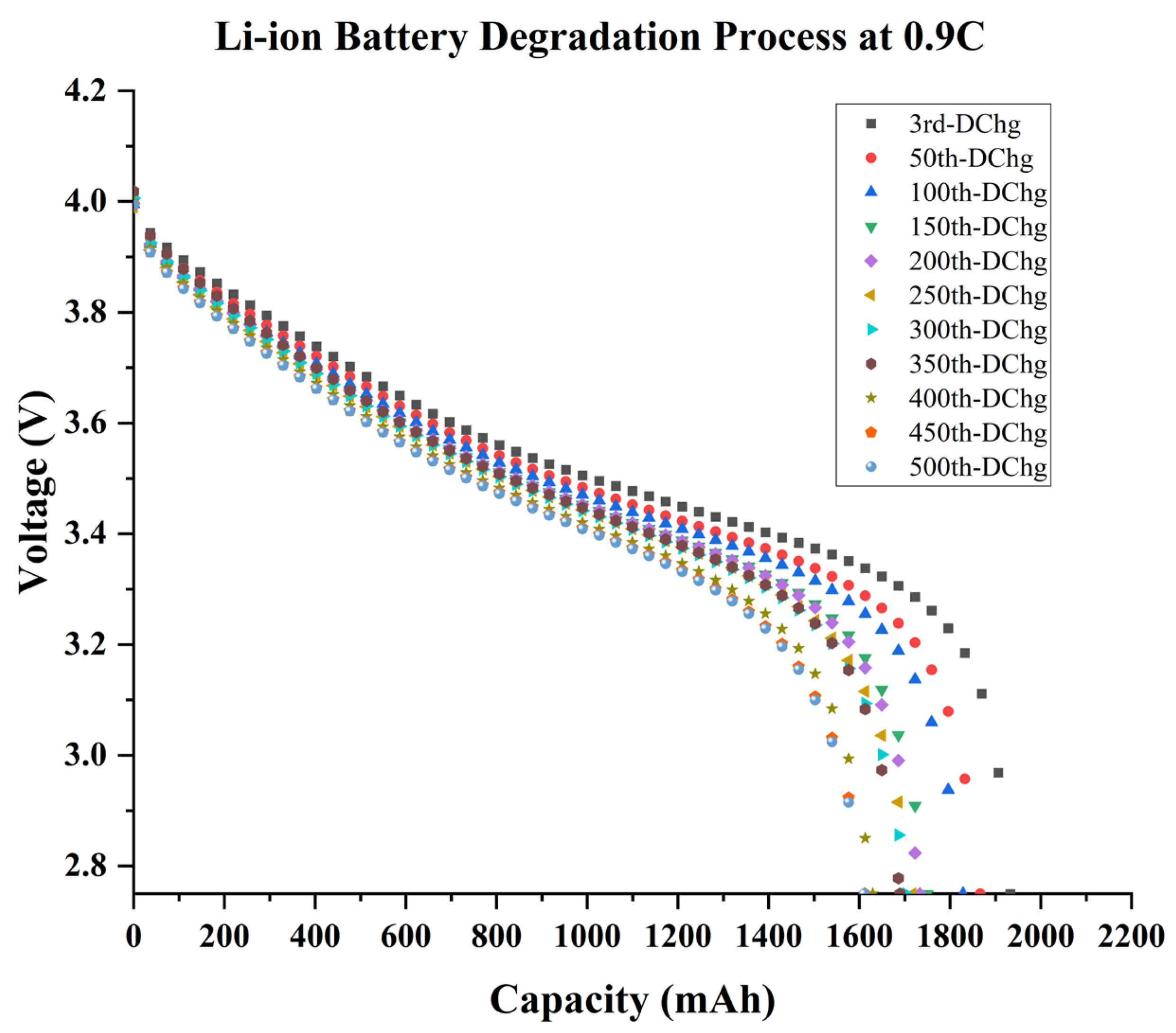
Batteries 09 00093 g004
Figure 5. The battery degradation process at 0.9 C-rate for 500 cycles, where degradation is shown every 50 cycles.
Batteries 09 00093 g005
Figure 6. The battery degradation process at 1.3 C-rate for 500 cycles, where degradation is displayed every 50 cycles.
Batteries 09 00093 g006
Figure 7. The battery degradation process at 1.6 C-rate for 500 cycles, where degradation is shown every 50 cycles.
Batteries 09 00093 g007
Figure 8. Comparison of battery degradation model performance with experimental and simulated data for individual battery capacity fades at 0.9C, 1.3C, and 1.6C.
Batteries 09 00093 g008
Figure 9. Selection of the permanent hidden layer with the FNN network based on the least-error values MAE (%), MSE (%) and RMSE (%) at hidden layers ranged from (3–10).
Batteries 09 00093 g009
Figure 10. The MAE (%), MSE (%), and RMSE (%) values, achieved with the FNN degradation model at three different accelerated discharging rates: 0.9C, 1.3C, and 1.6C.
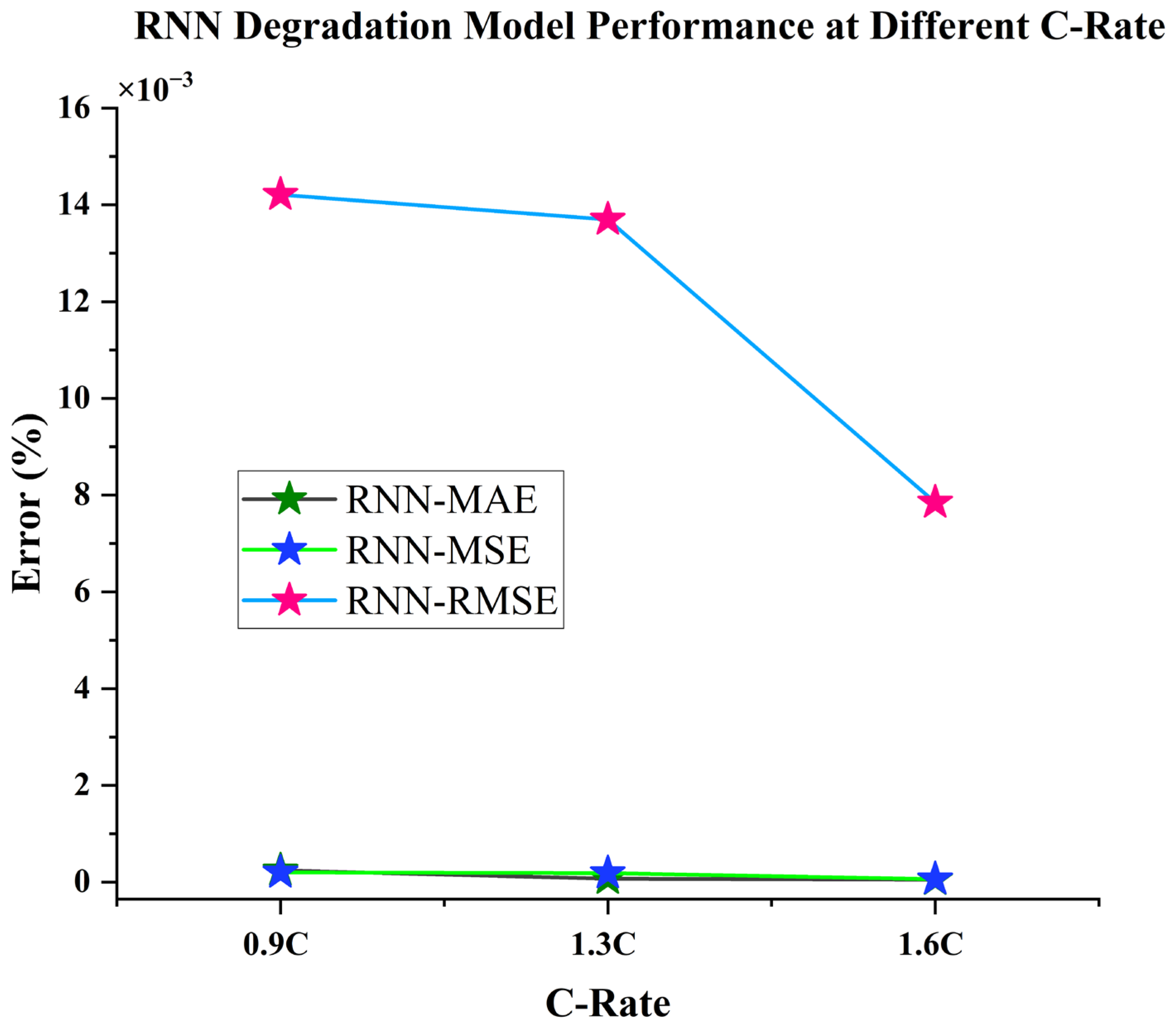
Batteries 09 00093 g010
Figure 11. The performance of the RNN degradation model based on the MAE (%), MSE (%), and RMSE (%) values at 3 separate accelerated discharge rates: 0.9C, 1.3C, and 1.6C.
Batteries 09 00093 g011
Figure 12. Comparison of the performance of RNN and FNN degradation models at 3 separate accelerated discharge rates: 0.9C, 1.3C, and 1.6C on the basis of MAE (%), MSE (%), and RMSE (%) values.
Batteries 09 00093 g012
Table 1. Battery specification of A18650 model of Hongli Li-ion battery.
Battery ParameterSpecification
Cell Voltage3.7 V
Nominal Capacity2200 mAh
Max Voltage4.2 V
Min Voltage2.5 V
Energy8.14 Wh
Table 2. Neware battery tester BTS4000 equipment specification.
Cycling BuilderNEWARE BTS4000
Cycling tester rating5 V/6 A
Test Channels0–8
Accuracy≥1%
Sample frequency10 Hz
Table 3. The degree of capacity fade at 0.9C, 1.3C, and 1.6C for every 50 cycles throughout its lifetime.
Cycle NumberCapacity Fade (%)
0.9C1.3C1.6C
504.081.986.25
1004.944.3320.78
1508.4611.3435.59
20010.4314.2560.87
25010.5722.5172.23
30011.3827.12-
35013.3932.84-
40013.4936.82-
45014.0741.31-
50015.1445.05-
Table 4. The MAE, MSE, and RMSE values with the hidden layers ranged between (3–10).
N.H. LayersMAEMSERMSE
32.26 × 10−81.43 × 10−81.92 × 10⁻⁴
41.21 × 10−63.12 × 10−41.76 × 10⁻⁴
51.64 × 10−71.45 × 10−53.84 × 10⁻³
61.54 × 10−94.51 × 10−82.12 × 10⁻⁴
71.67 × 10−89.92 × 10−83.15 × 10⁻⁴
81.31 × 10−98.17 × 10−99.04 × 10⁻⁵
95.14 × 10−92.77 × 10−61.01 × 10⁻³
104.98 × 10−94.91 × 10−91.67 × 10⁻³
Table 5. FNN degradation model performance based on MAE, MSE, and RMSE values at various discharge rates: 0.9C, 1.3C, and 1.6C.
C-RateMAEMSERMSE
0.9C 2.12 × 10−43.17 × 10−41.78 × 10⁻²
1.3C1.12 × 10−41.62 × 10−41.27 × 10−2
1.6C 4.49 × 10−51.04 × 10−41.02 × 10⁻²
Table 6. RNN degradation model performance based on MAE, MSE, and RMSE values at various discharge rates: 0.9C, 1.3C, and 1.6C.
C-RateMAEMSERMSE
0.9C2.44 × 10−42.02 × 10−41.42 × 10−2
1.3C7.03 × 10−51.88 × 10−41.37 × 10−2
1.6C5.27 × 10−56.16 × 10−57.85 × 10−3
Disclaimer/Publisher’s Note: The statements, opinions and data contained in all publications are solely those of the individual author(s) and contributor(s) and not of MDPI and/or the editor(s). MDPI and/or the editor(s) disclaim responsibility for any injury to people or property resulting from any ideas, methods, instructions or products referred to in the content.

