Article

A K-Value Dynamic Detection Method Based on Machine Learning for Lithium-Ion Battery Manufacturing

1
Sichuan New Energy Vehicle Innovation Center Co., Ltd., Yibin 644000, China
2
School of Vehicle and Mobility, Tsinghua University, Beijing 100084, China
3
SVOLT Energy Technology Co., Ltd., Changzhou 213200, China
4
Dr. Octopus Intelligent Technology (Shanghai) Co., Ltd., Shanghai 201800, China
*
Author to whom correspondence should be addressed.
Batteries 2023, 9(7), 346; https://doi.org/10.3390/batteries9070346
Submission received: 18 May 2023 / Revised: 17 June 2023 / Accepted: 21 June 2023 / Published: 27 June 2023

Abstract

:
During the manufacturing process of the lithium-ion battery, metal foreign matter is likely to be mixed into the battery, which seriously influences the safety performance of the battery. In order to reduce the outflow of such foreign matter defect cells, the production line universally adopted the K-value test process. In the traditional K-value test, the detection threshold is determined empirically, which has poor dynamic characteristics and probably leads to missing or false detection. Based on comparing the screening effect of different machine learning algorithms for the production data of lithium-ion cells, this paper proposes a K-value dynamic screening algorithm for the cell production line based on the local outlier factor algorithm. The analysis results indicate that the proposed method can adaptively adjust the detection threshold. Furthermore, we validated its effectiveness through the metal foreign matter implantation experiment conducted in the pilot manufacturing line. Experiment results show that the proposed method’s detection rate is improved significantly. The increase in the detection rate of foreign matter defects is beneficial to improving battery quality and safety.

1. Introduction

As the global energy shortage and environmental pollution are increasingly severe, electric vehicles that use electric energy as the power source instead of traditional fossil fuels have attracted more and more attention [1]. For the electric vehicle, the core is the battery. The lithium-ion battery is widely used in electric vehicles as the power source due to the advantages of high-energy density and a long cycle life, and so on [2,3]. However, in recent years, safety accidents related to electric vehicle power batteries have occurred frequently, especially battery spontaneous combustion and thermal runaway, which are kinds of accidents with severe consequences [4,5,6,7]. On the one hand, battery thermal runaway is related to battery abuses, such as overcharging, deformation, and high temperature [8,9,10]. On the other hand, it is related to the manufacturing defects of the battery itself. Relevant research shows that even under normal working conditions, manufacturing defects are likely to trigger the “self-induced, sudden-death-type” thermal runaway (SSTR) of lithium-ion batteries [11]. Therefore, the quality control and management of the product during the manufacturing process of lithium-ion batteries plays a significant role.
The lithium-ion cell manufacturing chain contains numerous intermediate stages, such as mixing, coating, drying, calendering, slitting, and stacking. During this complex process, various manufacturing defects are likely to occur [12,13,14,15,16], such as pinholes, agglomerations, and scratches in the electrode surface, significantly influencing the cell’s performance. However, the metal foreign matter defect is also a severe cell manufacturing defect, possibly caused by contaminants in manufacturing raw materials, metal fragments during electrode plate slitting or welding slag during electrode tab welding, etc. The metal foreign matter defect is most likely to cause the internal short circuit (ISC) inside the lithium-ion cell [17,18,19], mainly including two types of short circuits. One is the physical short circuit caused by the metal foreign matter directly puncturing the separator. The other is the chemical dissolution short circuit caused by the connection of the cathode and anode after dissolution-precipitation of metal particle contaminants. When the lithium-ion cell has an internal short circuit, the risk of thermal runaway might increase, and even battery spontaneous combustion would be triggered, endangering people’s lives. Therefore, the research on foreign matter defects of lithium-ion cells is currently a hotspot. Sun et al. investigated the mechanism of ISC caused by metal particle contaminants in the cell and the influences of this kind of defect on the electrical properties of the cell [20]. Qian et al. analyzed the chemical composition of impurity particles in the defective 18650-type cells and possible sources during manufacturing processes. They reported that impurities near the separator could pierce through the separator, potentially triggering ISC and thermal runaway [12]. Mohanty et al. studied the effect of implanted Al foil and Co-powder contaminants on the electrochemical performance of the coin cell. They found that metal particle contaminants may accelerate capacity degradation and lead to poor rate capability [21]. The above literature mainly focuses on the evolution mechanism of metal foreign matter defect cells but does not propose how to detect them.
Currently, there is not much research on detecting foreign matter defect cells. Most researchers concentrate on developing novel algorithms to monitor online whether there is an internal short circuit inside the lithium-ion cell based on real-time data from the vehicle or energy storage power station [22,23,24]. Undoubtedly, online monitoring of the operational status of the cell through the battery management system (BMS), to some degree, could reduce incidences of safety accidents induced by the foreign matter defect cell. However, it is more important to conduct quality control and improve the detection rate of defect cells during manufacturing. At present, there are many state-of-the-art methods for quality verification in lithium-ion cell manufacturing, such as visual checking by scanning electron microscopy (SEM), chemical analysis by energy dispersive X-ray spectroscopy (EDX), and so on [25]. Such destructive evaluations cannot meet the requirement of real-time detection in mass production. Several nondestructive methods are also used for quality inspection, including Raman spectroscopy, X-rays radiography, and computed tomography (CT). However, these methods are mainly applied to check electrode misalignment, electrode folding, coating defects, etc. [26]. So far, there are no relatively perfect and feasible solutions to the issue of detecting the foreign matter defect cell in the production line. Yi et al. attempted to use an ultrasonic nondestructive testing (NDT) technique to detect foreign matter defects inside a cell. However, the ability of this technology is restricted to the thickness and structure of the cell, as well as the morphology of the defect [27]. Fink et al. evaluated the impacts of various metal impurities on the electrochemical and thermal performance of the lithium-ion cell, including Fe, Cu, Mg, Al, and Si. Their findings imply that the coupling of electrochemical and thermal methods can be used to detect specific contaminants. However, the cells used in their study were coin cells and single-layer pouch cells made from the laboratory rather than prismatic lithium-ion cells manufactured from the actual production line [28]. Kong et al. reproduced the sudden spontaneous combustion (SSC) caused by foreign metal matter between the cell jelly roll and cell housing of the prismatic lithium-ion cell. They also discussed the influence of this kind of foreign matter defect on the safety performance of the cell. In addition, they also proposed corresponding warning methods, which could be used in the production line. However, the proposed method is primarily aimed at SSTR, and their research is not involved with the foreign metal matter between electrode plates [11]. Thus, it is necessary to develop a novel method for detecting the foreign matter defect cell and validate its effectiveness in the production line.
With the rapid development of AI technology and big data technology, machine-learning algorithms have also been applied to lithium-ion cells’ operation management and manufacturing management. As intelligent algorithms based on data, machine-learning algorithms have classification and prediction functions, which can be used to realize fault diagnosis and defect detection of the cell, avoiding complex mechanism-based modeling processes. The current researches are mainly about deploying various machine-learning algorithms in the BMS to realize online fault diagnosis of lithium-ion batteries [29,30,31], while there are few studies on applying these algorithms to the detection of defect cells in the production line. Against this backdrop, it is of great significance to make full use of big data of the production line and machine-learning algorithm to detect foreign matter defect cells, which helps to improve the intelligence level of lithium-ion cell manufacturing.
To this end, this paper proposes a novel K-value dynamic detection method based on machine learning and big data of the production line to detect foreign matter defect cells in the production line. The remainder of this paper is organized as follows: Section 2 introduces the relationship between the detection of foreign matter defect cells and K-value and analyzes shortcomings of the traditional K-value test process in the production line. Section 3 compares the performance of different anomaly detection algorithms based on big data of the production line. Section 4 introduces the proposed K-value dynamic detection method and analyses this method’s performances from different perspectives, then validates its effectiveness through the metal foreign matter implantation experiment conducted in the pilot production line. Section 5 provides a conclusion.

2. Foreign Matter Defect and K-Value Test

2.1. Relationship between Foreign Matter Defect and K-Value

It is one of the most common foreign matter defects that metal particle contaminants are introduced between the cathode and separator of lithium-ion cells. In this case, the ISC is likely to be triggered. The metal particle contaminant on the high-potential cathode dissolves and deposits on the anode. Eventually, because metal depositions directly connect the cathode and anode, the ISC occurs. The ISC is likely to cause abnormal self-discharge, namely, that the defect cell tends to have a higher self-discharge rate than the normal cells [20,32]. Therefore, monitoring the self-discharge rate is an effective method for detecting the foreign matter defect cell in the production line.
The K-value is one of the common indicators for evaluating the self-discharge rate of lithium-ion cells, which denotes the open circuit voltage (OCV) drop rate. Since the OCV corresponds with the battery state of charge (SOC), the OCV drop rate can reflect the self-discharge rate. The K-value is calculated as the following equation [33,34]:
K = O C V 1 O C V 2 t 1 t 2
where OCV1 is the open circuit voltage at t1 time, OCV2 is the open circuit voltage at t2 time.
Therefore, during the manufacturing of lithium-ion cells, the K-value test is carried out to detect cells with a high self-discharge rate to reduce the outflow rate of defect cells. The process of testing the K-value in the production line is shown in Figure 1. After the formation process and high-temperature aging process, lithium-ion cells are rested at room temperature (25 °C). In this process, the open circuit voltage of a cell at different times is measured and recorded, then the K-value of this cell is obtained.

2.2. Disadvantages of Traditional K-Value Test

It is generally known that the relationship between OCV and SOC of the lithium-ion cell is not linear, which means that the self-discharge characteristics of a cell at different OCVs are not the same. If a cell starts to self-discharge over a period at different OCVs, the measured K-values are also different. During the actual K-value test process, the OCV of each cell is different. Therefore, besides the K-value, the OCV value also needs to be used, reflecting K-value distributions at different OCVs. Based on this, cells with abnormal K-values are detected as the following steps: (i) Firstly, after obtaining the K-value and OCV value of cells, the upper and lower thresholds of the K-value and OCV value are determined based on the empirical distribution of them; (ii) Then, the cell whose OCV-K-value is beyond the given threshold will be judged as abnormal. Herein, the OCV value refers to the open circuit voltage at the starting time. The schematic diagram of a certain batch of lithium-ion cells’ OCV-K distribution in the pilot cell manufacturing line is shown in Figure 2, in which the ideal detection threshold of OCV-K is marked with the green dashed box. As shown in Figure 2a, it is clear that those points with excessively large K-values and points with excessively large or low OCV are outside the green dashed box and will be judged as outlier points. In this case, there is neither misjudgment nor omission.
In the mass production of lithium-ion cells, due to the effects of various factors such as batch fluctuation of raw materials, wearing of the equipment, fine-tuning of process parameters, change of ambient temperature, adjustment of production line workers, the distribution of OCV-K is not static but dynamic. As a result, although the traditional K-value test based on the static boundary mentioned above is easy to conduct, it has some disadvantages. For instance, as shown in Figure 2b, the mean values of OCV and K both change, but the set threshold remains unchanged. In this case, some outlier points (marked with the pink shadow in Figure 2b) enter into the green dashed box, leading to the omission, while some inlier points (those which are marked with the blue shadow in Figure 2b) move outside the green dashed box, leading to misjudgment. Furthermore, from Figure 2c, it is evident that with the change of production consistency in the production line, the variance values of OCV and K alter. In this case, some outlier points (marked with the pink shadow in Figure 2c) enter into the green dashed box, leading to omission. Therefore, it is necessary to improve this traditional K-value test process.

3. Performance of Different Anomaly Detection Algorithms

3.1. Algorithm Description

From discussions in the previous section, if the distribution of OCV-K changes, the traditional K-value detection method cannot adaptively adjust the detection threshold, which is likely to cause misjudgment and omission. Thus, how to choose the detection threshold to detect these defect cells is vitally important. If the threshold is set to low, the false detection will occur, while if the threshold is set to high, the missing detection will occur. Thus, a dynamic K-value detection mechanism is required. Detecting cells with poor K-values can be regarded as identifying outlier points in the unlabeled dataset. In other words, the unlabeled training dataset contains outliers. Therefore, this is an outlier detection problem, one of the two types of anomaly detection problems. In order to solve this problem, different anomaly detection algorithms are studied in this section, including the Isolation Forest (iForest) algorithm, One-Class Support Vector Machine (OCSVM) algorithm, and Local Outlier Factor (LOF) algorithm, which represent different principles of anomaly detection algorithms. One of the advantages of the three anomaly detection algorithms above is that they are unsupervised machine-learning algorithms and suitable for handling the unlabeled dataset.

3.1.1. Isolation Forest Algorithm

The Isolation Forest algorithm is a model-based anomaly detection algorithm, similar to the Random Forest algorithm in principle [35]. The basic principle of this algorithm is to split the data points using a proper binary tree structure called the isolation tree (iTree) until each data point is separated from the rest of the data points. A proper binary tree means each node has zero or two child nodes. In this process, the less the number of splitting required to isolate a sample, thus the greater the probability that this sample is an outlier. The basic steps of employing the iForest algorithm to screen outliers in dataset X are as follows:
  • Step 1 Training dataset
The iForest is an ensemble of n iTrees. In this stage, the construction process of each iTree is as follows: (i) θ samples are selected randomly from dataset X as the subset X’. Then, this subset is put into the root node. (ii) Randomly select an attribute from a list of attributes in the subset X’ and a split value p between the max and min values of the selected attribute. (iii) The split value p divides subset X’ into two parts. If data is less than p in the selected attribute, it will be moved to the left subtree of the current tree node, or it will be moved to the right subtree. (iv) Repeat the above procedures in the child nodes until each data point lies on a node alone or the height of this iTree reaches the specified value.
  • Step 2 Computing anomaly score
In this step, firstly, let each instance x in dataset X traverse each iTree constructed above. Then, record the path length of x in each iTree, defined as the number of edges x traversing an iTree from the root node to an external node. Based on this, compute the anomaly score s(x, θ) of each data point x in dataset X, according to the following equation [35,36]:
s ( x , θ ) = 2   E ( h ( x ) ) c ( θ )
where θ is the size of the subset X’ used to build an iTree, h(x) is the path length of the data point x, E(h(x)) is the average of h(x) of all iTrees in the iForest, c(θ) is the normalization factor, describing the average path length of the iTree given θ, computed as the following equation [35]:
c ( θ ) = 2 H ( θ 1 ) 2 ( θ 1 ) / θ       i f   θ > 2                               1                                                   i f   θ = 2                               0                                                   o t h e r w i s e
where H(θ − 1) is the harmonic number and can be estimated by ln(θ − 1) + 0.5772156649 (Euler’s constant).
For an outlier point, it will be likely to traverse a shorter path and get a higher anomaly score [37].
  • Step 3 Identifying the outlier point based on the threshold
After computing the anomaly scores of all data points in dataset X, whether the data point x is an outlier point can be determined by the following equation:
f ( x ) = sgn ( s ( x ) Q 100 % contamination )
where f(x) is the decision function (if f(x) = −1, the data point x is the outlier point), contamination is the proportion of outlier points in dataset X, Q100%-contamination is the (100%-contamination)th percentile of anomaly scores of all data points.

3.1.2. One-Class Support Vector Machine Algorithm

As a variant of binary-class Support Vector Machine (SVM), the One-Class Support Vector Machine algorithm (OCSVM) is often used for anomaly detection. Traditional SVM aims to find a linear hyperplane in the feature space that separates positive samples from negative samples with a maximum margin [38]. If original data are not linearly separable, these data can be mapped into higher dimensional feature space via a non-linear kernel function, equivalent to constructing a non-linear classifier in the original data space. In contrast to SVM, OCSVM is trained on the single-class dataset, indicating that all training data points are unlabeled. Therefore, in OCSVM, the origin in the feature space is regarded as the negative sample point. Based on this, the OCSVM algorithm attempts to construct a linear hyperplane that maximizes the separation between the origin and all samples in the feature space [38,39]. Then, whether a data point is an outlier is determined by its location relative to the hyperplane. The main steps of using the OCSVM algorithm to identify outliers in dataset X are as follows:
  • Step 1 Training dataset
In order to find the aforementioned linear hyperplane, we need to solve the following optimization problem [39,40]:
min 1 2 w 2 + 1 ν N i = 1 N ξ i ρ s . t . w ϕ ( x i ) ρ ξ i     ξ i 0
where w and ρ are, respectively, the normal vector and the offset of the hyperplane, N and ν are, respectively, the number of all samples and fraction of outliers in the dataset X, ξi is the slack variable of the ith data point, φ is the mapping function that maps original sample points from X to new feature space.
Similar to binary-class SVM, the quadratic optimization problem of (5) can be solved using Lagrange multipliers and the dual form of the Lagrangian. The detailed solution process can be referred to in [39,40]. In order to construct a non-linear classifier in the original input space, a kernel function is used to map original sample points into a higher dimensional feature space. In this paper, the Gaussian-kernel function is used.
  • Step 2 Identifying the outlier points
Then, after the hyperplane of the OCSVM is calculated, a non-linear boundary is created. The sample points belonging to the normal class will lie within the boundary, whereas the abnormal class will be on the other side. Whether the data point x is an outlier can be determined by the following equation:
f ( x ) = sign ( ( w ϕ ( x i ) ) ρ )
where f(x) is the decision function, if f(x) = −1, the data point x is the outlier point.

3.1.3. Local Outlier Factor Algorithm

The Local Outlier Factor algorithm is an anomaly detection algorithm based on the local density rather than global density, the most distinct advantage of which is that the detected outlier is the local outlier with respect to its neighborhoods [41]. The core idea of the LOF algorithm is to assign to each sample in the dataset a local outlier factor that can quantify the degree of outlier-ness of this sample. If the LOF value of a sample is beyond the specific threshold, it will be classified as an outlier. The main steps of employing the LOF algorithm to detect outliers in dataset X are as follows:
  • Step 1 Computing the local reachability density
The local reachability density of the data point x in dataset X, denoted by lrdk(x), is defined as [41,42]:
l r d k ( x ) = 1 / o N k ( x ) r e a c h _ d i s t k ( o , x ) N k ( x )
where Nk(x) and |Nk(x)| are, respectively, the collection of k-nearest neighbors of the data point x in dataset X and the size of this collection. reach_distk(o,x) is the reachability distance of the data point x with respect to the data point o and defined as:
r e a c h _ d i s t k ( o , x ) = max d k ( o ) , d ( o , x )
where d(o,x) is the Euclidean distance between the data points x and o, dk(o) is the k-distance of the data point o, equal to the maximum Euclidean distance from the data point o to its k-nearest neighbors.
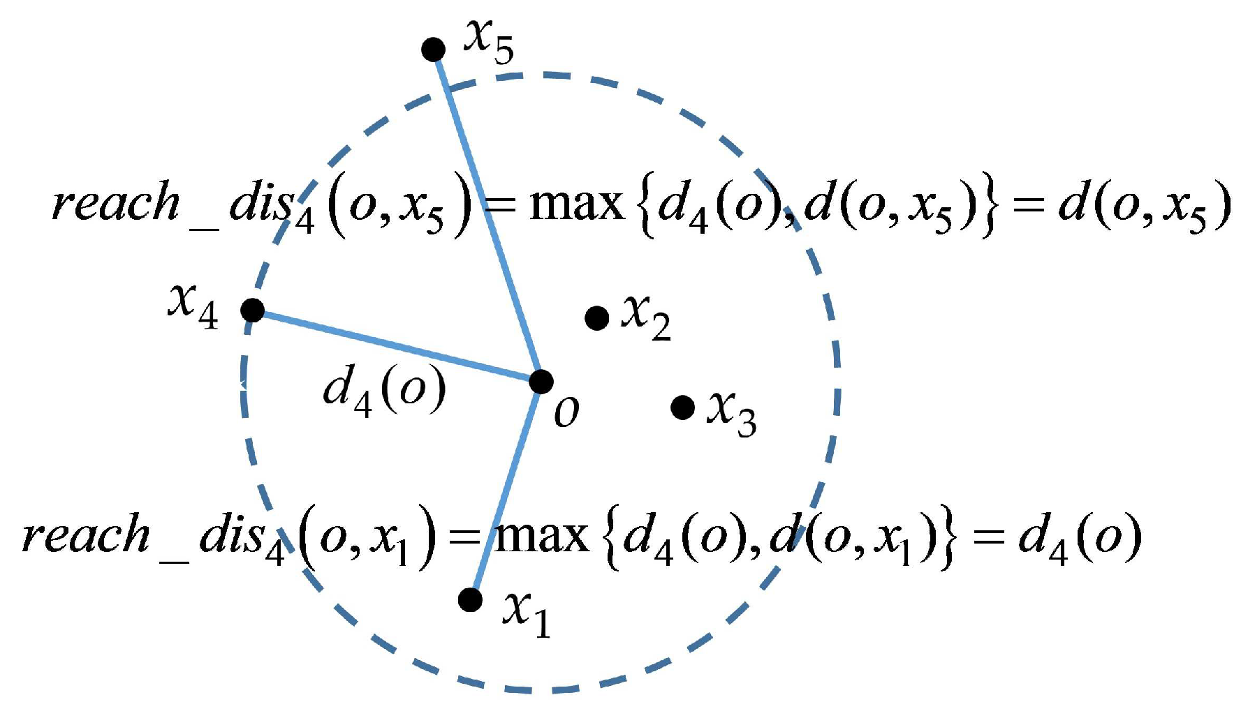
The diagram of the reachability distance is shown in Figure 3. For k = 4, the k-nearest neighbors of the data point o consist of the points in and on the blue circle, so the k-distance of the data point o(d4(o)) is equal to d(o,x4). Clearly, because d(o,x1) is smaller than d4(o), reach_dist4(o,x1) is equal to d4(o), whereas because d(o,x5) is larger than d4(o), reach_dist4(o,x5) is equal to d(o,x5).
  • Step 2 Computing the local outlier factor
The local outlier factor of the data point x is denoted by LOFk(x) and computed by the following equation [41,42]:
L O F k ( x ) = o N k ( x ) l r d k ( o ) l r d k ( x ) N k ( x )
where, lrdk(x) and lrdk(o) are the local reachability density of the data points x and o.
  • Step 3 Identifying the outlier point based on the threshold
After computing the local outlier factors of all data points in dataset X, whether the data point x is an outlier can be determined by the following equation:
f ( x ) = sgn ( L O F k ( x ) Q 100 % contamination )
where f(x) is the decision function.(if f(x) = −1, the data point x is the outlier point), contamination is the proportion of outlier points in dataset X, Q100%-contamination is the (100%-contamination)th percentile of local outlier factors of all data points.

3.2. Comparison of Different Algorithms’ Performance

The cell used in this study is a prismatic lithium-ion cell for electric vehicles, in which the detailed parameters are shown in Table 1. The dataset in this study is the OCV-K dataset for the prismatic lithium-ion cell, which consists of two features, namely, the K-value and OCV value at the starting time of the K-value test. The acquisition process of the above two features is shown in Figure 1. The OCV measurement device measures the OCV values at the beginning and end of room-temperature aging. After that, the K-value is calculated and recorded. With the help of the manufacturing execution system, the K-values and OCV values of 3000 lithium-ion cells are randomly collected to produce an OCV-K dataset. Then, three anomaly detection algorithms are tested on this OCV-K dataset to detect the cells with abnormal K-values.
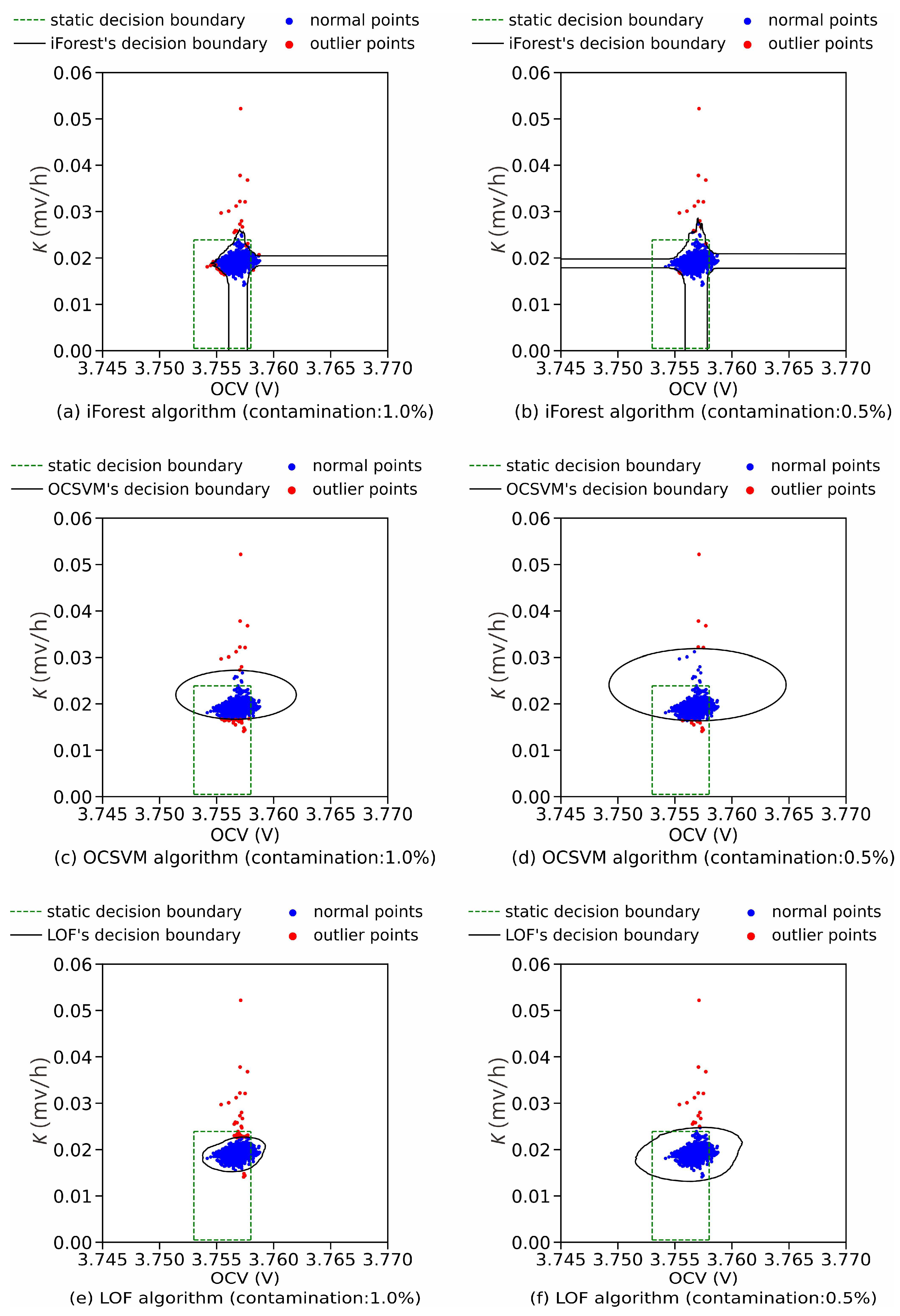
The detection results of three anomaly detection algorithms are shown in Figure 4, where the decision boundaries of different algorithms are also displayed. Herein, the parameter “contamination” denotes the fraction of outlier points in the dataset. As shown in Figure 4a, when the contamination value is set to 1%, those points with a significantly large K-value are outside the decision boundary and detected by the iForest algorithm. However, some points with a large K-value on the top of the normal points’ region, which are expected to be outliers, are inside the decision boundary and wrongly judged as normal. Additionally, some points near the left edge of the normal points’ region, which are expected to be normal, are wrongly judged as outliers. Thus, the phenomena of both omission and misjudgment happen. As shown in Figure 4b, when the contamination value is set to 0.5%, the envelope range of the decision boundary is enlarged, and the points judged as outliers are reduced. At the same time, a few points near the left edge of the normal points’ region are also wrongly judged as outliers.
As shown in Figure 4c, the OCSVM algorithm can also detect those points with a significantly large K-value when the contamination value is set to 1%. However, some points with a large K-value on the top of the normal points’ region, which are expected to be judged as outliers, are wrongly judged as normal. Besides missing detection, many points near the lower edge of the normal points’ region are misjudged as outliers. Figure 4d also shows that when the contamination value decreases to 0.5%, the envelope range of the OCSVM algorithm’s decision boundary is enlarged. In this case, the points judged as outliers become fewer. Although the contamination value is set to lower, some points near the lower edge of the normal points’ region are still misjudged as outliers.
As shown in Figure 4e, the performance of LOF algorithms significantly improves, compared with the two algorithms above. When the contamination value is set to 1%, the decision boundary is very consistent with the boundary formed by the region of ideal inlier points, and those points with a large K-value are almost detected without misjudgment and omission. From Figure 4f, similar to the two algorithms above, the envelope range of the LOF algorithm’s decision boundary is enlarged, and the number of outliers detected by the LOF algorithm is reduced with the decrease in the contamination value.
From the above comparisons, the LOF algorithm has the best performance in detecting the outlier points in the OCV-K dataset with the lowest degree of omission and misjudgment.
The green dashed box in Figure 4 denotes the decision boundary of the traditional K-value testing with the upper limit of the K-value 0.0239 mV/h. From Figure 4, it can be seen that because the decision boundary of the traditional K-value testing process cannot change adaptively as OCV-K distribution alters; many points fall outside the decision boundary, leading to severe false detection. After the anomaly detection algorithms based on machine learning are introduced, the decision boundary can change adaptively, improving the detection method’s dynamic performance.

4. K-Value Dynamic Detection Method Based on LOF

In the above section, the performances of different anomaly detection algorithms were analyzed, and we found that the LOF algorithm based on local density performs best. Therefore, in this section, a novel K-value dynamic detection method based on LOF is proposed for detecting cells with abnormal K-values. Unlike the traditional detection method, this new method can evaluate the outlier degree of each cell in the dataset and adjust the anomaly threshold adaptively.

4.1. Description of K-Value Dynamic Detection Method

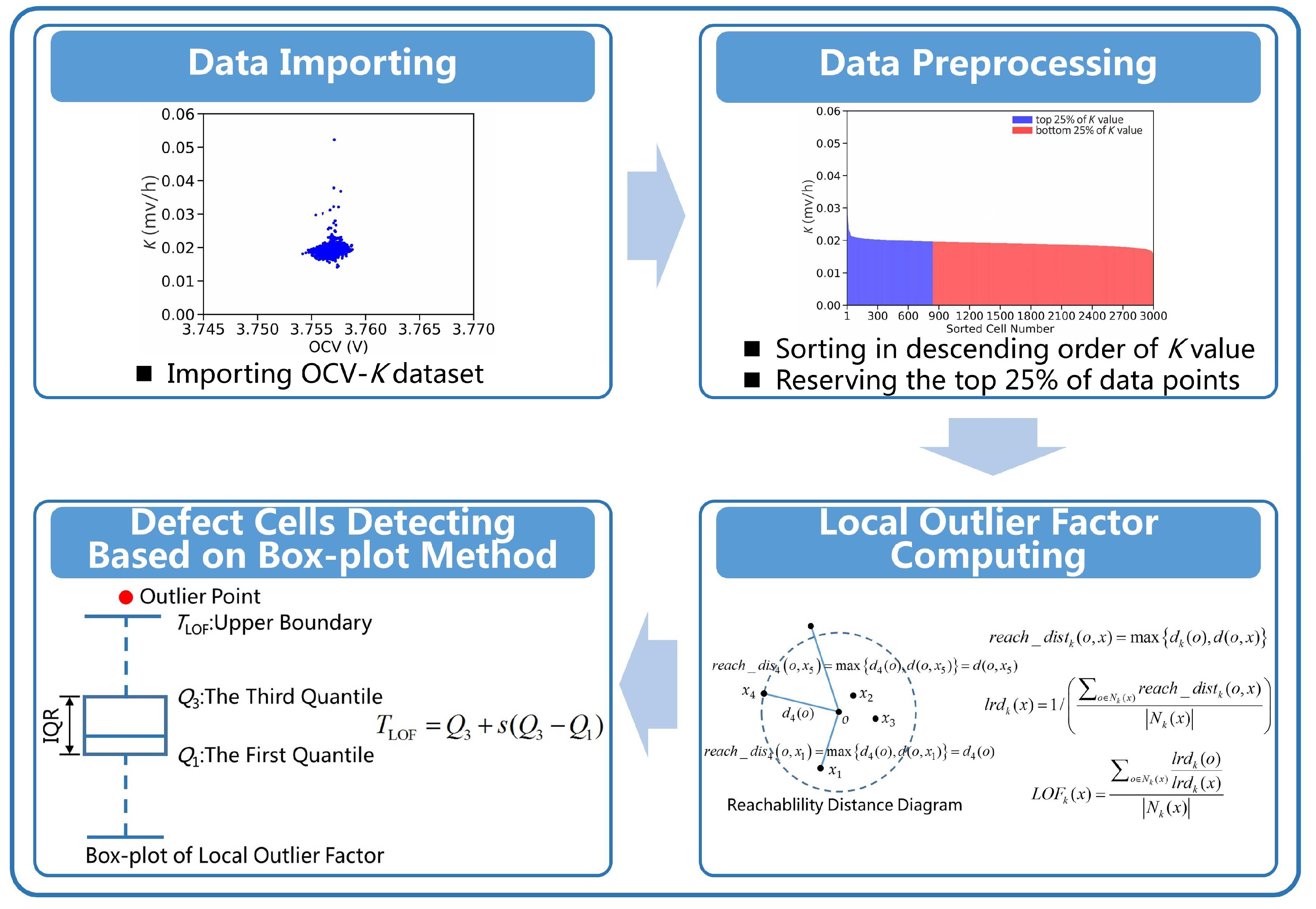
The flowchart of the proposed K-value dynamic detection method is shown in Figure 5. It is generally believed that the cell with a high K-value should be abnormal, while the cell with a low K-value should be normal. Therefore, to prevent false detection, the imported OCV-K dataset of lithium-ion cells needs to be preprocessed. Firstly, sort all samples in the OCV-K dataset in descending order of K-value. Then, the samples in the top 25% of the K-value are reserved as the input for evaluating the outlier degree in the next step. Based on this, the local outlier factors of samples from preprocessed OCV-K dataset are computed by the calculation method in the LOF algorithm. The local outlier factor is an indicator of the outlier degree.
Once the local outlier factor of a sample exceeds the set threshold, the corresponding cell will be considered an abnormal cell. In the previous section, the LOF algorithm is used under the condition that the defect rate is set to a specific value. In this case, the number of detected defect cells is also constant. However, the defect rate is dynamic in the cell manufacturing process, affected by the level of production conformity. If the production conformity is well controlled, outlier points decrease, meaning fewer cells will be judged as abnormal. Similarly, the poor level of production conformity makes outlier points increase, which means that more cells will be judged as abnormal. Therefore, the threshold of the local outlier factor is determined by the box-plot method [43]. As shown in Figure 5, if the local outlier factor of a data point is beyond the upper boundary, this data point is judged as an outlier point. The detection threshold, denoted by TLOF, is computed as the following equation:
T LOF = Q 3 + s ( Q 3 Q 1 )
where Q3 and Q1 are, respectively, the third and first quartile of LOF of all samples from the preprocessed OCV-K dataset; s is the scale factor and the LOF threshold changes with the adjustment of s.

4.2. Performance Analysis of K-Value Dynamic Detection Method

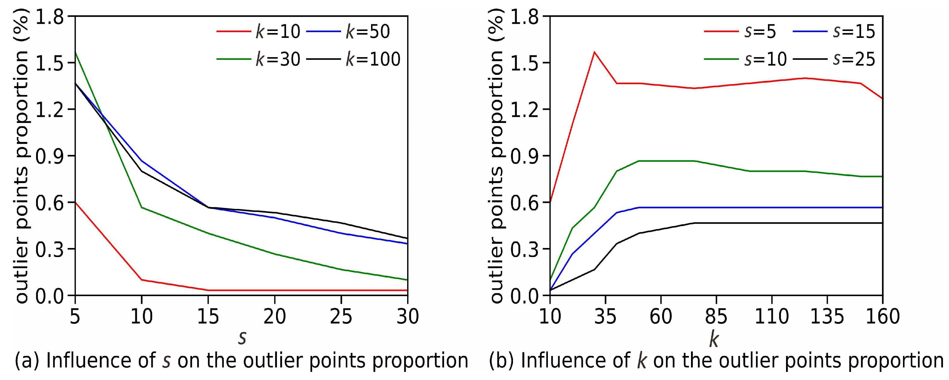
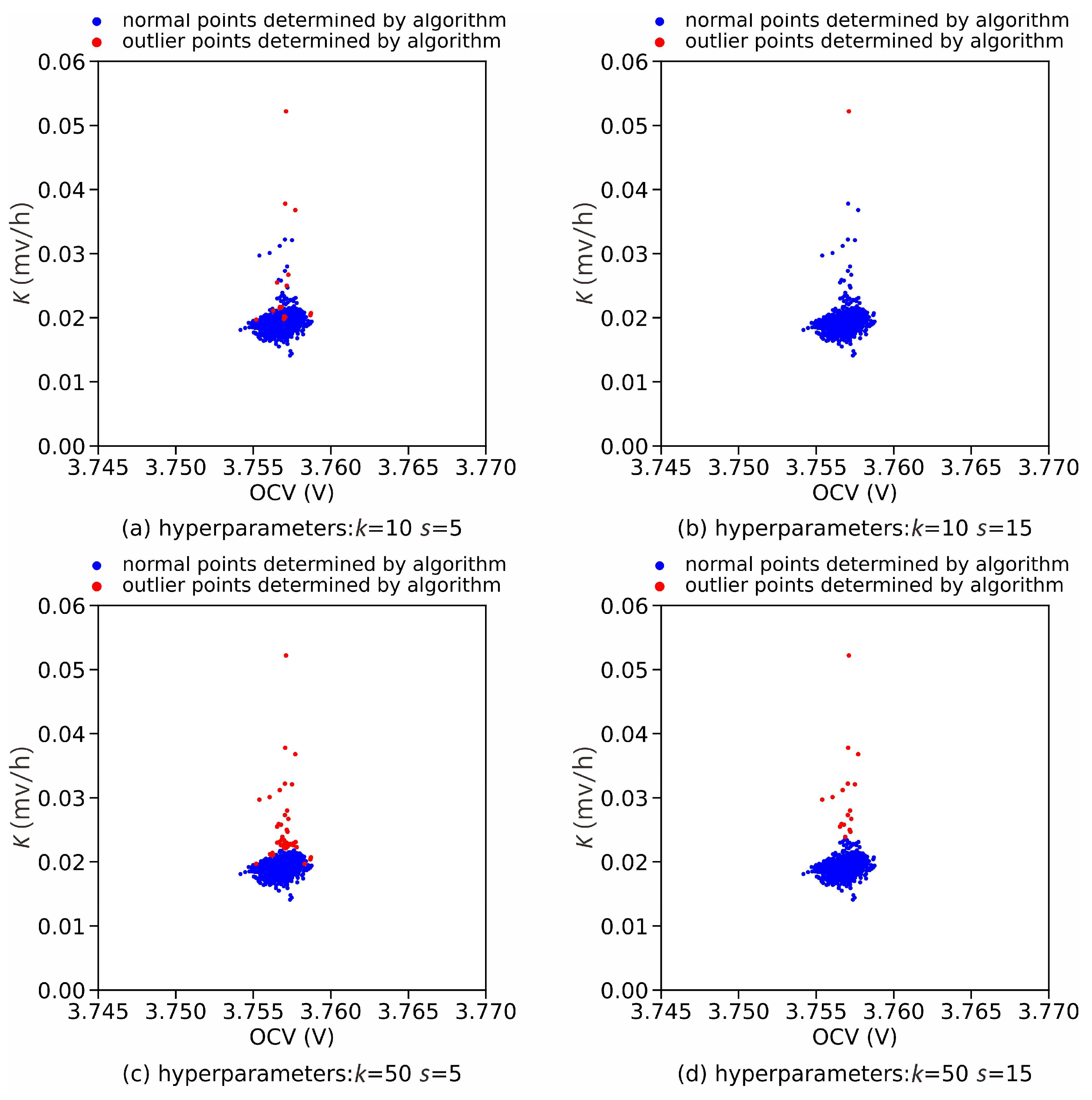
Firstly, the OCV-K dataset of lithium-ion cells, with the size of 3000 in the previous section, was used to analyze the effect of the hyperparameters on the detection results. Equations (9) and (11) show that the detection method has two hyperparameters, k and s. The hyperparameter k means that the LOF of a sample point is calculated based on the k-nearest neighbors of this sample point. The hyperparameter s is a scale factor to adjust the detection threshold. The influence of hyperparameters on outlier points’ proportion is shown in Figure 6. It can be seen that the proportion of cells judged as abnormal declines as the hyperparameter s increases. In contrast, this proportion rises with the hyperparameter k increases and tends to be stable when k increases to around 50.
The detection results of the K-value dynamic detection method with different combination of hyperparameters is shown in Figure 7. From Figure 7a, when s = 5 and k = 10, some data points with high-outlier degrees cannot be detected, resulting in omission. In this case, the performance of the K-value dynamic detection method is poor. Then, s remains constant, and k increases. As shown in Figure 7c,d, when s = 5, k = 50, and s = 5, k = 100, detection results are the same without missing detection. From Figure 7b, when s = 15 and k = 10, the missing detection occurs again. Then, s remains at 15, and k increases. As shown in Figure 7d,f, when s = 15, k = 50, and s = 15, k = 100, there is no missing detection, similar to the results shown in Figure 7c,d. The primary reason for this is because the local outlier factor of one data point is relative to its k-nearest neighbors. For example, suppose cluster A contains several evenly distributed outlier points outside a cluster of normal points. Intuitively, if k is too small, the k-nearest neighbors of a datapoint p in cluster A will all belong to cluster A. Thus, point p is not an outlier relative to its k-nearest neighbors. Therefore, the hyperparameter k cannot be set to a too small value, or severe missing detection will occur. In addition, Figure 7 also shows that when k remains constant and s increases, fewer data points are judged as outliers, which indicates that adjusting the hyperparameter s can change the sensitivity of the K-value dynamic detection method to outlier points.
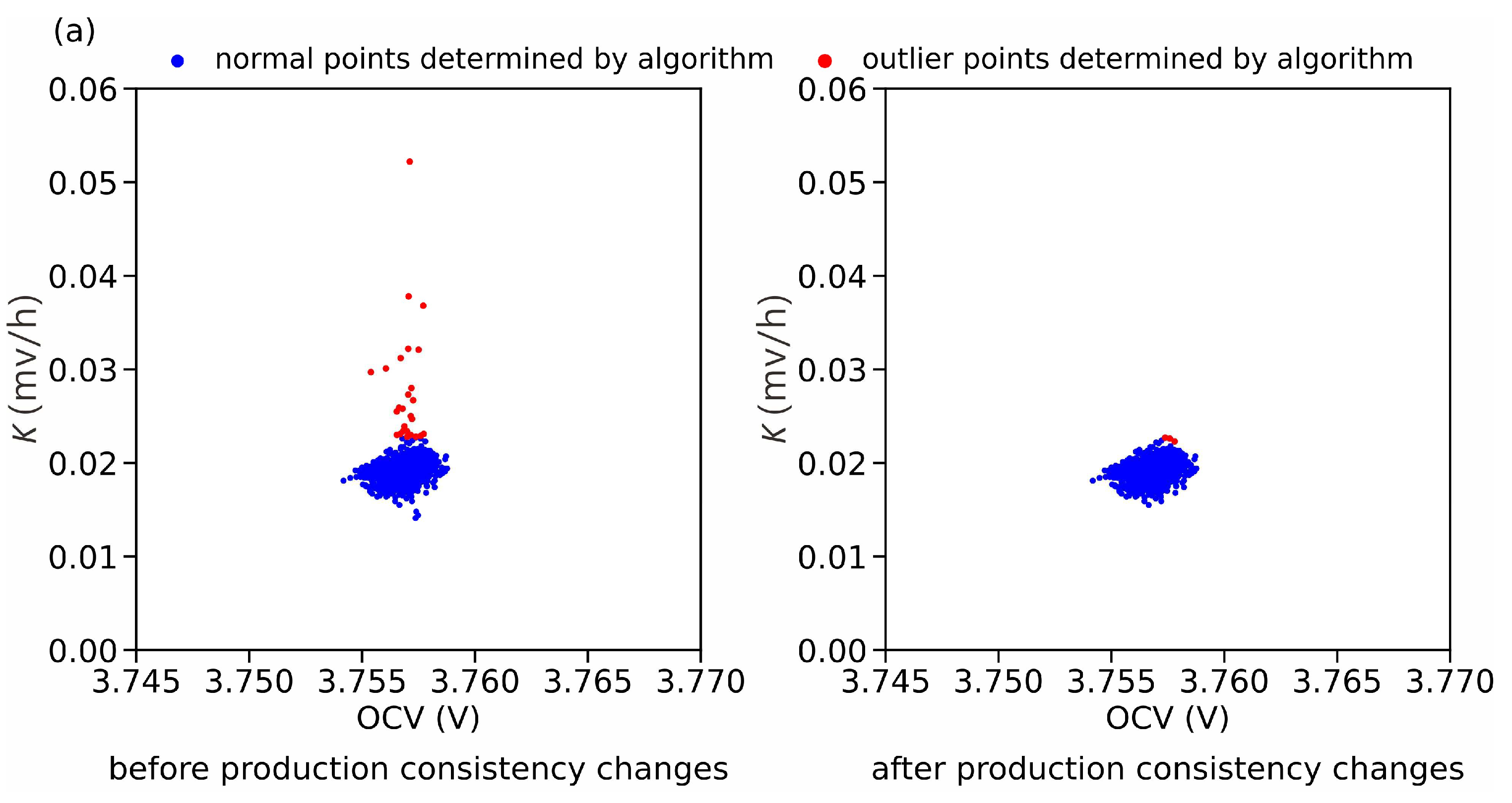
Furthermore, two sets of parallel tests were carried out, respectively, using two OCV-K datasets, with the size of 3000, to test if the proposed K-value dynamic detection method applies to the scenario of the production consistency change. In this study, the hyperparameters k and s are, respectively, set to 75 and 10. In order to simulate OCV-K distribution after the production consistency changes, some outlier points in the OCV-K dataset are screened out. From Figure 8a, production consistency is poor before the change, and 26 cells are judged as defective, accounting for 0.87% of all test samples. In contrast, after production consistency is improved; three cells are judged as defective, accounting for 0.1% of all test samples.
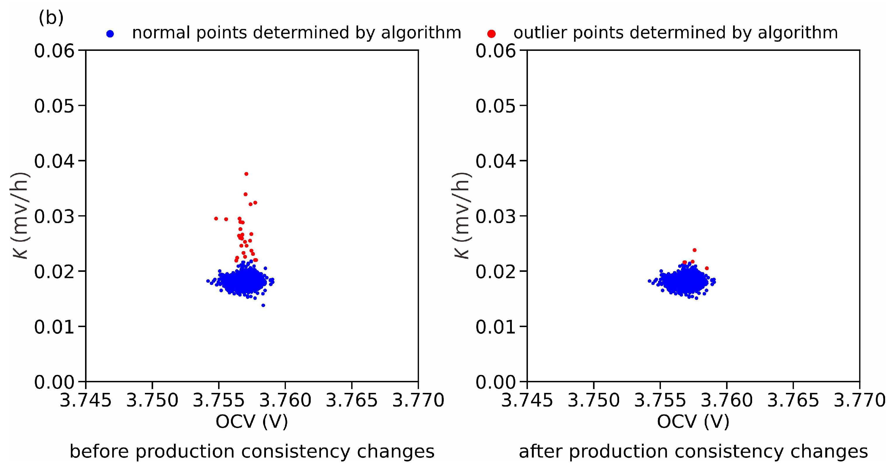
Similarly, as shown in Figure 8b, 28 cells are judged as defective before production consistency changes, accounting for 0.93% of all test samples. In contrast, five cells are judged as defective after the change of production consistency, accounting for 0.17% of all test samples.
The test results above indicate that the proposed K-value dynamic detection method can deal with the case of production consistency change during cell manufacturing, namely, that the number of cells judged as defective decreases adaptively as the level of production consistency rises.

4.3. Experimental Validation

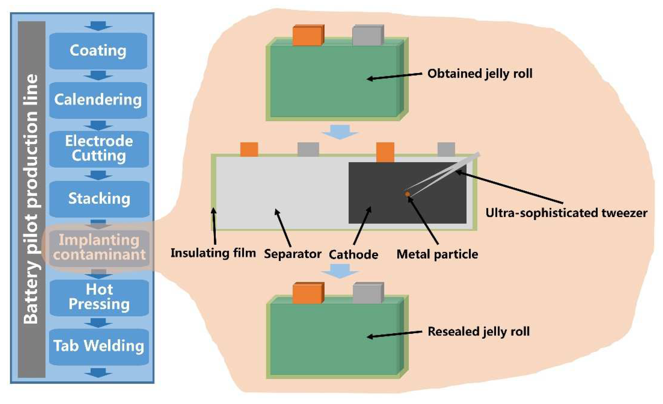
The analysis above is based on the unlabeled OCV-K dataset, so it is necessary to verify further the effectiveness of the proposed K-value dynamic detection method on the labeled OCV-K dataset. In order to generate a labeled OCV-K dataset, the foreign matter defect cells are produced by implanting metal particles into lithium-ion cells in the pilot production line. It is for simulating the generation process of the foreign matter defect cell during the actual manufacturing. Then, through the MES (Manufacturing Execution System) of the production line, the labeled OCV-K dataset is obtained, including 31 foreign matter defect cells and 3351 normal cells. The cell used in the experiment is still a prismatic lithium-ion cell, the detailed information of which is listed in Table 1. The experimental process is shown in Figure 9. After the stacking process, a specific number of jelly rolls are randomly obtained from the pilot production line to conduct the implantation of metal particles with different sizes. Moreover, only one metal particle is implanted on the cathode plate surface of each collected jelly roll with the help of the ultra-sophisticated tweezer. The jelly roll with a metal contaminant is resealed and reintroduced into the pilot production line when implantation is conducted. Some information related to cell state, such as type and size of foreign matter, are recorded in the MES to be traced later. In this study, the material of the metal particle is copper, and its size is measured with a digital microscope. The diameters of all 31 metal particles range from 150 μm to 300 μm.
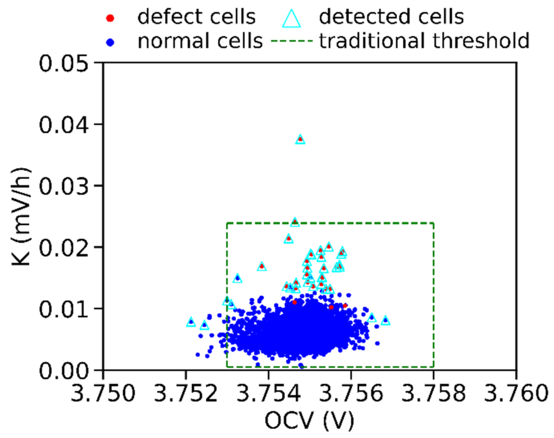
Next, the proposed K-value dynamic detection method is used to test the labeled OCV-K dataset above. The detection results of foreign matter defect cells with different sizes of metal particles are listed in Table 2. It can be seen that the K-value dynamic detection method proposed in this paper detects 28 of the 31 foreign matter defect cells. As shown in Figure 10, in this OCV-K scatter plot, the distribution position of three omitted defect cells (red data points not enclosed by a triangle) is closer to the region of normal cells. Therefore, these three defect cells have lower LOF values, which is the main reason for missing detection.
In this study, the detection rate and accuracy are used as the indicators to evaluate the effectiveness of the method for detecting defect cells, computed as the following equation:
detection   rate = TP TP + FN accuracy = TP + TN TP + TN + FP + FN
where TP is the true positive value, denoting the number of abnormal cells which are correctly classified as abnormal, FN is the false negative value, denoting the number of abnormal cells which are wrongly classified as normal, FP is the false positive value, denoting the number of normal cells which are wrongly classified as abnormal, and TN is the true negative value, denoting the number of normal cells which are correctly classified as normal.
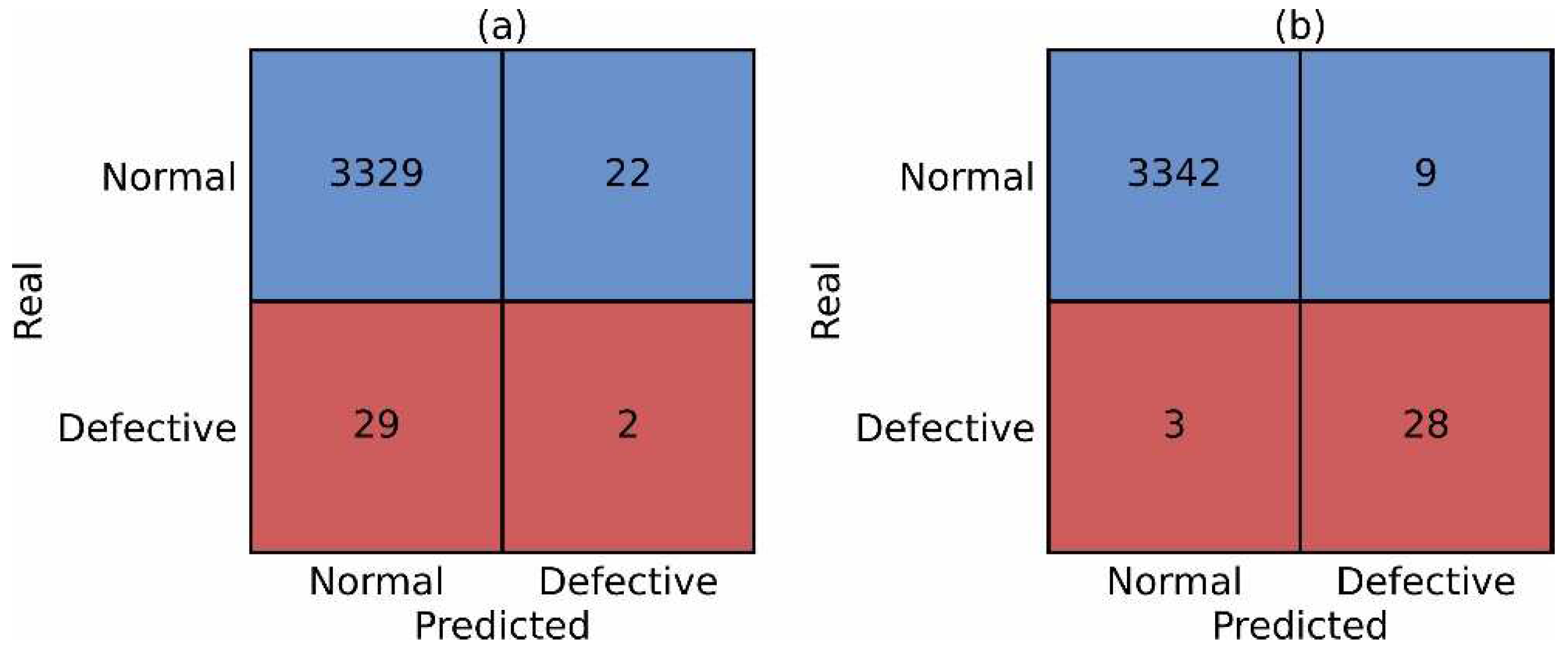
The confusion matrices of traditional K-value detection and K-value dynamic detection method proposed in this paper are shown in Figure 11. From Figure 11a, only two defect cells are detected by the traditional method with a detection rate of 6.5%. From Figure 11b, when the proposed K-value dynamic detection method is used, the TP value increases significantly, and the detection rate reaches 90.3%. Meanwhile, the number of cells incorrectly classified as abnormal decreases to nine, accounting for 0.27% of all cells. According to Equation (11), the accuracy is also calculated as 99.7%. The experiment result indicates that the performance of the proposed K-value dynamic detection method is superior to the traditional detection method.

5. Conclusions

The metal foreign matter mixed into the cell is a stubborn problem in the cell manufacturing process. It is generally believed that metal contaminants in a cell can cause ISC, increasing its self-discharge rate. The K-value test process is widely used in cell production lines to screen defective cells, but this method has shortcomings. The anomaly threshold is empirically set to fixed values, probably leading to omission or misjudgment. Therefore, an adaptive intelligent detection mechanism is needed to deal with complex and changeable cell manufacturing industrial scenarios.
In this paper, the K-value detection is improved by introducing machine learning. Firstly, the screening effects of different machine learning algorithms on defect cells at the production line were compared and analyzed, including the iForest algorithm, the OCSVM algorithm, and the LOF algorithm. The results show that the screening effect of the LOF algorithm is the best, and there is no obvious phenomenon of an erroneous judgment. Then, a novel K-value dynamic detection method based on LOF is proposed for the production line, and the screening effect of the algorithm is verified by using the OCV-K data sets. The analysis results indicate that when the distribution of OCV-K changes, the proposed method can adaptively adjust the detection threshold.
Finally, in order to verify the detection effect of the proposed method on the real foreign matter defect cells, we artificially made some defect cells on the pilot production line. Based on this, we used the real-time production data of the production line to verify the proposed method. The experiment results show that the proposed method’s detection rate reaches 90.3%, which is superior to the traditional detection method. Therefore, the proposed detection method in this paper can more effectively detect the foreign matter defect cells in the production line and reduce erroneous judgment and reword, which is of great significance for improving cell safety, reducing production costs, and increasing productivity.

Author Contributions

Conceptualization, X.K.; methodology, X.K. and H.Z.; software, Y.Y. and H.Z.; validation, Y.Y. and J.H.; investigation, X.H. and H.Z.; resources, Y.L. and X.Z.; data curation, X.Z., Y.Y. and Y.L.; writing—original draft preparation, H.Z.; writing—review and editing, X.K. and X.H.; visualization, H.Z.; supervision, M.O. and L.L.; funding acquisition, X.K. and M.O. All authors have read and agreed to the published version of the manuscript.

Funding

This research was supported by the National Natural Science Foundation of China under Grant No. 52107226, the China Postdoctoral Science Foundation under Grant No. 2020TQ0167, and the Science and Technology Project of Yibin Sanjiang New Area under Grant No. 2023SJXQSXZJ001.

Data Availability Statement

Not applicable.

Conflicts of Interest

The authors declare no conflict of interest.

References

  1. Kong, D.; Wang, G.; Ping, P.; Wen, J. A Coupled Conjugate Heat Transfer and CFD Model for the Thermal Runaway Evolution and Jet Fire of 18650 Lithium-Ion Battery under Thermal Abuse. eTransportation 2022, 12, 100157. [Google Scholar] [CrossRef]
  2. Hu, G.; Huang, P.; Bai, Z.; Wang, Q.; Qi, K. Comprehensively Analysis the Failure Evolution and Safety Evaluation of Automotive Lithium Ion Battery. eTransportation 2021, 10, 100140. [Google Scholar] [CrossRef]
  3. Wang, H.; Xu, H.; Zhang, Z.; Wang, Q.; Jin, C.; Wu, C.; Xu, C.; Hao, J.; Sun, L.; Du, Z.; et al. Fire and Explosion Characteristics of Vent Gas from Lithium-Ion Batteries after Thermal Runaway: A Comparative Study. eTransportation 2022, 13, 100190. [Google Scholar] [CrossRef]
  4. Held, M.; Tuchschmid, M.; Zennegg, M.; Figi, R.; Schreiner, C.; Mellert, L.D.; Welte, U.; Kompatscher, M.; Hermann, M.; Nachef, L. Thermal Runaway and Fire of Electric Vehicle Lithium-Ion Battery and Contamination of Infrastructure Facility. Renew. Sustain. Energy Rev. 2022, 165, 112474. [Google Scholar] [CrossRef]
  5. Wang, Q.; Mao, B.; Stoliarov, S.I.; Sun, J. A Review of Lithium Ion Battery Failure Mechanisms and Fire Prevention Strategies. Prog. Energy Combust. Sci. 2019, 73, 95–131. [Google Scholar] [CrossRef]
  6. Lai, X.; Yao, J.; Jin, C.; Feng, X.; Wang, H.; Xu, C.; Zheng, Y. A Review of Lithium-Ion Battery Failure Hazards: Test Standards, Accident Analysis, and Safety Suggestions. Batteries 2022, 8, 248. [Google Scholar] [CrossRef]
  7. Peiyan, Q.I.; Jie, Z.M.; Da, J.; Kai, Y.; Jianling, L.; Yilin, L.; Fei, G.; Hao, L. Combustion Characteristics of Lithium–Iron–Phosphate Batteries with Different Combustion States. eTransportation 2022, 11, 100148. [Google Scholar] [CrossRef]
  8. Zhou, Z.; Zhou, X.; Cao, B.; Yang, L.; Liew, K.M. Investigating the Relationship between Heating Temperature and Thermal Runaway of Prismatic Lithium-Ion Battery with LiFePO4 as Cathode. Energy 2022, 256, 124714. [Google Scholar] [CrossRef]
  9. Jones, C.; Li, B.; Tomar, V. Determining the Effects of Non-Catastrophic Nail Puncture on the Operational Performance and Service Life of Small Soft Case Commercial Li-Ion Prismatic Cells. eTransportation 2021, 8, 100109. [Google Scholar] [CrossRef]
  10. Liu, J.; Wang, Z.; Bai, J. Influences of Multi Factors on Thermal Runaway Induced by Overcharging of Lithium-Ion Battery. J. Energy Chem. 2022, 70, 531–541. [Google Scholar] [CrossRef]
  11. Kong, X.; Lu, L.; Yuan, Y.; Sun, Y.; Feng, X.; Yang, H.; Zhang, F.; Zhang, J.; Liu, X.; Han, X.; et al. Foreign Matter Defect Battery and Sudden Spontaneous Combustion. eTransportation 2022, 12, 100170. [Google Scholar] [CrossRef]
  12. David, L.; Ruther, R.E.; Mohanty, D.; Meyer, H.M.; Sheng, Y.; Kalnaus, S.; Daniel, C.; Wood, D.L. Identifying Degradation Mechanisms in Lithium-Ion Batteries with Coating Defects at the Cathode. Appl. Energy 2018, 231, 446–455. [Google Scholar] [CrossRef]
  13. Qian, G.; Monaco, F.; Meng, D.; Lee, S.-J.; Zan, G.; Li, J.; Karpov, D.; Gul, S.; Vine, D.; Stripe, B.; et al. The Role of Structural Defects in Commercial Lithium-Ion Batteries. Cell Rep. Phys. Sci. 2021, 2, 100554. [Google Scholar] [CrossRef]
  14. Choudhary, N.; Clever, H.; Ludwigs, R.; Rath, M.; Gannouni, A.; Schmetz, A.; Hülsmann, T.; Sawodny, J.; Fischer, L.; Kampker, A.; et al. Autonomous Visual Detection of Defects from Battery Electrode Manufacturing. Adv. Intell. Syst. 2022, 4, 2200142. [Google Scholar] [CrossRef]
  15. Li, Y.; Fu, X.; Wang, Y.; Zhong, W.-H.; Li, R. “See” the Invisibles: Inspecting Battery Separator Defects via Pressure Drop. Energy Storage Mater. 2019, 16, 589–596. [Google Scholar] [CrossRef]
  16. Kim, N.; Byun, S.; Jin, D.; Dzakpasu, C.B.; Park, S.H.; Lee, H.; Hong, S.-T.; Lee, Y.M. Electrode Alignment: Ignored but Important Design Parameter in Assembling Coin-Type Full Lithium-Ion Cells. J. Electrochem. Soc. 2022, 169, 023502. [Google Scholar] [CrossRef]
  17. Zhang, G. Internal Short Circuit Mechanisms, Experimental Approaches and Detection Methods of Lithium-Ion Batteries for Electric Vehicles: A Review. Renew. Sustain. Energy Rev. 2021, 141, 110790. [Google Scholar] [CrossRef]
  18. Nakajima, H.; Kitahara, T. Diagnosis Method to Detect the Incorporation of Metallic Particles in a Lithium Ion Battery. ECS Trans. 2015, 68, 59–74. [Google Scholar] [CrossRef]
  19. Grabow, J.; Klink, J.; Benger, R.; Hauer, I.; Beck, H.-P. Particle Contamination in Commercial Lithium-Ion Cells—Risk Assessment with Focus on Internal Short Circuits and Replication by Currently Discussed Trigger Methods. Batteries 2022, 9, 9. [Google Scholar] [CrossRef]
  20. Sun, Y.; Yuan, Y.; Lu, L.; Han, X.; Kong, X.; Wang, H.; Ouyang, M.; Gao, P.; Zheng, H.; Wang, K. A Comprehensive Research on Internal Short Circuits Caused by Copper Particle Contaminants on Cathode in Lithium-Ion Batteries. eTransportation 2022, 13, 100183. [Google Scholar] [CrossRef]
  21. Mohanty, D.; Hockaday, E.; Li, J.; Hensley, D.K.; Daniel, C.; Wood, D.L. Effect of Electrode Manufacturing Defects on Electrochemical Performance of Lithium-Ion Batteries: Cognizance of the Battery Failure Sources. J. Power Source 2016, 312, 70–79. [Google Scholar] [CrossRef] [Green Version]
  22. Yuan, H. Early Stage Internal Short Circuit Fault Diagnosis for Lithium-Ion Batteries Based on Local-Outlier Detection. J. Energy Storage 2023, 57, 106196. [Google Scholar] [CrossRef]
  23. Feng, X. Detecting the Internal Short Circuit in Large-Format Lithium-Ion Battery Using Model-Based Fault-Diagnosis Algorithm. J. Energy Storage 2018, 18, 26–39. [Google Scholar] [CrossRef]
  24. Chen, A.; Zhang, W.; Zhang, C.; Wang, Z.; Fan, X. A Novel Al–Cu Internal Short Circuit Detection Method for Lithium-Ion Batteries Based on on-Board Signal Processing. J. Energy Storage 2022, 52, 104748. [Google Scholar] [CrossRef]
  25. Kong, L.; Aalund, R.; Alipour, M.; Stoliarov, S.I.; Pecht, M. Evaluating the Manufacturing Quality of Lithium Ion Pouch Batteries. J. Electrochem. Soc. 2022, 169, 040541. [Google Scholar] [CrossRef]
  26. McGovern, M.E.; Bruder, D.D.; Huemiller, E.D.; Rinker, T.J.; Bracey, J.T.; Sekol, R.C.; Abell, J.A. A Review of Research Needs in Nondestructive Evaluation for Quality Verification in Electric Vehicle Lithium-Ion Battery Cell Manufacturing. J. Power Source 2023, 561, 232742. [Google Scholar] [CrossRef]
  27. Yi, M.; Jiang, F.; Lu, L.; Hou, S.; Ren, J.; Han, X.; Huang, L. Ultrasonic Tomography Study of Metal Defect Detection in Lithium-Ion Battery. Front. Energy Res. 2021, 9, 806929. [Google Scholar] [CrossRef]
  28. Fink, K.E.; Polzin, B.J.; Vaughey, J.T.; Major, J.J.; Dunlop, A.R.; Trask, S.E.; Jeka, G.T.; Spangenberger, J.S.; Keyser, M.A. Influence of Metallic Contaminants on the Electrochemical and Thermal Behavior of Li-Ion Electrodes. J. Power Source 2022, 518, 230760. [Google Scholar] [CrossRef]
  29. Zhao, Y.; Liu, P.; Wang, Z.; Zhang, L.; Hong, J. Fault and Defect Diagnosis of Battery for Electric Vehicles Based on Big Data Analysis Methods. Appl. Energy 2017, 207, 354–362. [Google Scholar] [CrossRef]
  30. Jiang, J.; Li, T.; Chang, C.; Yang, C.; Liao, L. Fault Diagnosis Method for Lithium-Ion Batteries in Electric Vehicles Based on Isolated Forest Algorithm. J. Energy Storage 2022, 50, 104177. [Google Scholar] [CrossRef]
  31. Samanta, A.; Chowdhuri, S.; Williamson, S.S. Machine Learning-Based Data-Driven Fault Detection/Diagnosis of Lithium-Ion Battery: A Critical Review. Electronics 2021, 10, 1309. [Google Scholar] [CrossRef]
  32. Liu, Z.; He, H.; Xie, J.; Wang, K.; Huang, W. Self-Discharge Prediction Method for Lithium-Ion Batteries Based on Improved Support Vector Machine. J. Energy Storage 2022, 55, 105571. [Google Scholar] [CrossRef]
  33. Zimmerman, A.H. Self-Discharge Losses in Lithium-Ion Cells. IEEE Aerosp. Electron. Syst. Mag. 2004, 19, 19–24. [Google Scholar] [CrossRef]
  34. Shan, H.; Cao, H.; Xu, X.; Xiao, T.; Hou, G.; Cao, H.; Tang, Y.; Zheng, G. Investigation of Self-Discharge Properties and a New Concept of Open-Circuit Voltage Drop Rate in Lithium-Ion Batteries. J. Solid State Electrochem. 2022, 26, 163–170. [Google Scholar] [CrossRef]
  35. Liu, F.T.; Ting, K.M.; Zhou, Z.-H. Isolation-Based Anomaly Detection. ACM Trans. Knowl. Discov. Data 2012, 6, 3. [Google Scholar] [CrossRef]
  36. Tao, X.; Peng, Y.; Zhao, F.; Zhao, P.; Wang, Y. A Parallel Algorithm for Network Traffic Anomaly Detection Based on Isolation Forest. Int. J. Distrib. Sens. Netw. 2018, 14, 155014771881447. [Google Scholar] [CrossRef] [Green Version]
  37. Chabchoub, Y.; Togbe, M.U.; Boly, A.; Chiky, R. An In-Depth Study and Improvement of Isolation Forest. IEEE Access 2022, 10, 10219–10237. [Google Scholar] [CrossRef]
  38. Mahadevan, S.; Shah, S.L. Fault Detection and Diagnosis in Process Data Using One-Class Support Vector Machines. J. Process Control 2009, 19, 1627–1639. [Google Scholar] [CrossRef]
  39. Schölkopf, B.; Platt, J.C.; Shawe-Taylor, J.; Smola, A.J.; Williamson, R.C. Estimating the Support of a High-Dimensional Distribution. Neural Comput. 2001, 13, 1443–1471. [Google Scholar] [CrossRef]
  40. Huang, G.; Chen, J.; Liu, L. One-Class SVM Model-Based Tunnel Personnel Safety Detection Technology. Appl. Sci. 2023, 13, 1734. [Google Scholar] [CrossRef]
  41. Breunig, M.M.; Kriegel, H.-P.; Ng, R.T.; Sander, J. LOF: Identifying Density-Based Local Outliers. In Proceedings of the 2000 ACM SIGMOD International Conference on Management of Data, Dallas, TX, USA, 15–18 May 2000; pp. 93–104. [Google Scholar] [CrossRef]
  42. Fan, Z.; Zi-xuan, X.; Ming-hu, W. Fault Diagnosis Method for Lithium-Ion Batteries in Electric Vehicles Using Generalized Dimensionless Indicator and Local Outlier Factor. J. Energy Storage 2022, 52, 104963. [Google Scholar] [CrossRef]
  43. Morales, C.; Giraldo, R.; Torres, M. Boxplot Fences in Proficiency Testing. Accredit. Qual. Assur. 2021, 26, 193–200. [Google Scholar] [CrossRef]
Figure 1. The process of testing the K-value in the cell production line.
Batteries 09 00346 g001
Figure 2. The schematic diagram of lithium-ion cells’ OCV-K distribution in the pilot cell manufacturing line: (a) case 1, (b) case 2, (c) case 3.
Batteries 09 00346 g002
Figure 3. The diagram of the reachability distance (for k = 4).
Batteries 09 00346 g003
Figure 4. The detection results of three anomaly detection algorithms.
Batteries 09 00346 g004
Figure 5. The flowchart of the K-value dynamic detection method.
Batteries 09 00346 g005
Figure 6. Influence of hyperparameters on outlier points proportion.
Batteries 09 00346 g006
Figure 7. Detection results of the K-value dynamic detection method with different combinations of hyperparameters.
Batteries 09 00346 g007aBatteries 09 00346 g007b
Figure 8. Detection results of the K-value dynamic detection method before and after production consistency changes: (a) test 1, (b) test 2.
Batteries 09 00346 g008aBatteries 09 00346 g008b
Figure 9. Illustration of the process of implanting metal particle contaminant into the cell.
Batteries 09 00346 g009
Figure 10. OCV-K scatter plot of the labeled experiment dataset.
Batteries 09 00346 g010
Figure 11. Confusion matrices of (a) the traditional K-value detection method and (b) the proposed K-value dynamic detection method.
Batteries 09 00346 g011
Table 1. Parameters of the prismatic lithium-ion cell.
ParametersValues
Nominal capacity (Ah)114
Cathode materialNCM
Anode materialGraphite
Charging cutoff voltage (V)4.2
Discharging cutoff voltage (V)2.8
Energy density (Wh/kg)227
Length/Height/Thickness (mm)147.5/105.8/2.3
Table 2. Detection result of defect cells with different diameters of metal particles.
The Diameter of the Metal Particle150 μm200 μm250 μm300 μm
Number of defect cells8887
Number of detected defect cells6886
Disclaimer/Publisher’s Note: The statements, opinions and data contained in all publications are solely those of the individual author(s) and contributor(s) and not of MDPI and/or the editor(s). MDPI and/or the editor(s) disclaim responsibility for any injury to people or property resulting from any ideas, methods, instructions or products referred to in the content.