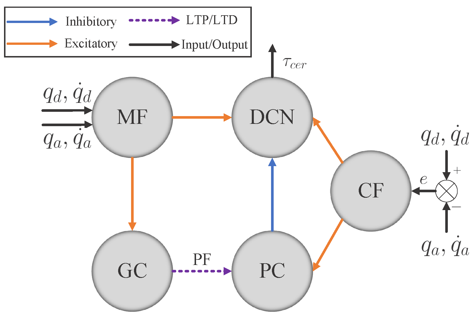
3.2.1. Cerebellum-like SNN
In this paper, the cerebellum module is implemented with SpikingJelly [
31], which is an open-source deep learning framework for SNN and has been used for exploring the applications of bio-inspired SNN in many aspects [
32,
33,
34]. The cerebellum-like SNN described in
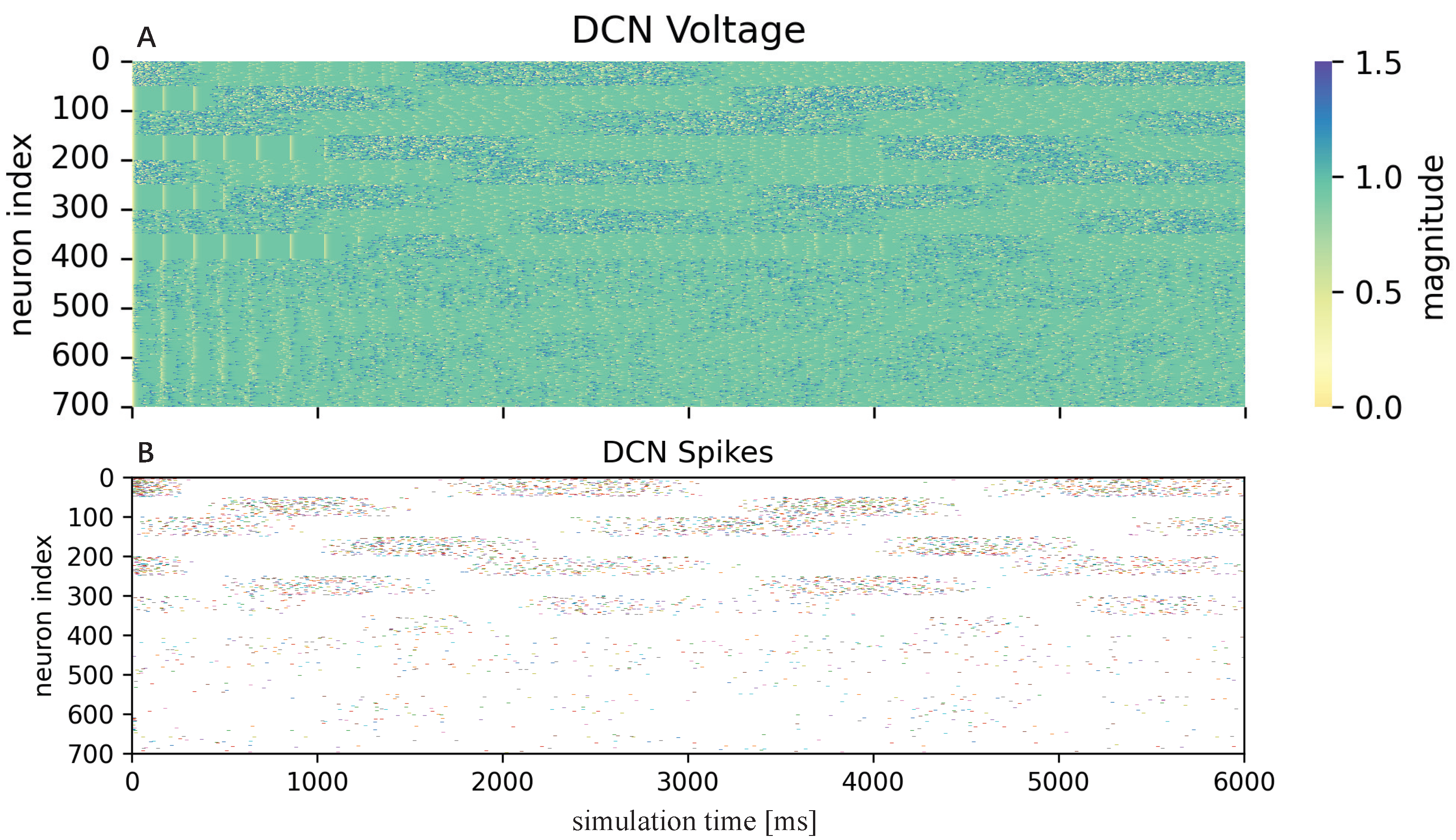
Figure 2 consists of five layers: MFs, GCs, PCs, CFs, and DCN. All of them are divided into seven microcomplexes, each one for controlling a robot joint. In the MF–GC, CF–PC, CF–DCN, and PC–DCN connections, the seven microcomplexes are indeed independent, where the MF–GC, CF–PC, and CF–DCN connections act like encoders. However, the neurons from MFs to DCN and GCs to PCs are all fully connected, which means the seven microcomplexes are dependent. The MF–DCN connection generates a constant membrane voltage changing to both positive and negative torque neurons in DCN, which helps in reducing the noise influence. The GC–PC connection is where STDP learns the dynamic mechanism of the robot from the command information encoded in MF and the error information encoded in CF and improves the control effects of the cerebellum-like SNN. The following part will introduce how to implement the five layers in detail.
The MF layer has 40 spiking neurons per microcomplex, 280 in total, translating the analog information to spikes. For each joint, the 40 neurons are divided into four subgroups for encoding feedback and desired joint positions and velocities, respectively, with ten neurons each. For an analog value
a with interval
, one spike
among the 10 neurons will be fired when
Therefore, 4 neurons per joint and 28 in total will be active at each time step. Every combination of four spikes is uniquely connected to one of 10,000 neurons per microcomplex in the GC layer with the excitatory synapse, represented by a positive weight
. All the neurons in the MF layer are concatenated together, fully connecting to the neurons in the DCN layer with excitatory synapse weight
.
CF layer modifies the error between the desired and actual trajectories per joint to spikes with 100 spiking neurons per microcomplex. The front half of the 100 neurons are dedicated to the forward movement of each joint, and the back half are for joint reversing, which mimics the interaction between agonist and antagonist muscles in human movement. The normalized error value
of each joint is given as
where
are the desired and actual joint position and velocity, respectively, and
are the upper and lower bounds of
j-th joint position and velocity. Poisson encoding is applied depending on the error value of each joint to obtain the spikes
, which can be expressed as
In order to be consistent with the joint movement, only up to half of the neurons of the CF layer will be active per microcomplex, which means if
,
; otherwise,
. Each neuron in the CF layer is connected one-to-one with each neuron in the PC layer and DCN layer with excitatory synapse weights
and
, respectively, also indicating the two other layers have the same number of neurons with the CF layer.
Neurons in the GC, PC, and DCN layers are all modeled as discrete-time LIF neurons to approximate the dynamics of the continuous-time LIF neurons. The membrane potential discrete-time charging function of the LIF neuron is
where
is the voltage leaking time constant and
is the input from synapses. To avoid confusion,
is used to represent the membrane potential after neuronal charging but before neuronal firing at time
t,
is the membrane potential after neuronal firing, and
is the reset value of membrane potential. The reset function of the membrane potential
depending on the firing state is
The firing state of the LIF neuron is described as
where
is the firing threshold. Therefore, a LIF neuron will fire a spike when the membrane potential
reaches the firing threshold. All the configuration parameters of LIF neurons are summarized in
Table 1.
The control mechanism of the cerebellum module is learned at the GC–PC connections by adjusting the synapses in PFs with the STDP mechanism. The trace method [
35] is used to implement STDP and avoid recording all the firing times of presynaptic and postsynaptic neurons described in Equation (
4). The update of synapse weight at time
t with the trace method is
where indices
indicate the presynaptic and postsynaptic neurons, respectively,
are functions constraining how weight changes, and
are the traces of the presynaptic and postsynaptic neurons that track their firing. The updated functions of the traces are
where
are the time constants of the presynaptic and postsynaptic neurons, similar to the leakage of LIF neurons.
in both Equations (
16) and (
17) are the firing states of the presynaptic and postsynaptic neurons.
Receiving excitatory synapses from the GC and CF layers, the neurons in the PC layer are activated and then one-to-one connected to the neurons in the DCN layer but with an inhibitory synapse, represented by a negative weight
.
Table 2 summarizes all the synapse weights. Finally, combining all the excitatory synapses from MF and CF layers and inhibitory synapses from the CF layer, the neurons in the DCN layer generate spikes, and then those spikes are mapped to joint torques
. The decode function of each microcomplex is as follows
where
is corresponding to the joint number,
is the mapping factor transforming the spikes to torques and is set as
.
3.2.2. CMCM with Deep Deterministic Policy Gradient
In this project, deep deterministic policy gradient (DDPG) [
36] algorithm as the RL implementation in CMCM is adopted to supervise the cerebellum module, based on a deep reinforcement learning library PFRL [
37]. DDPG is a model-free algorithm that learns the deterministic policy to the continuous action domain, as
where
is the action vector,
is the state vector, and
is the parameter of the policy network. The actions are interpreted as additional desired joint positions and added to the original position targets from the trajectory generator. The state vector
is spliced by the desired and actual joint positions and velocities.
In addition, an action-value function
is used in DDPG for describing the expected reward in Equation (
9) after taking an action
in state
. Considering the function approximators parameterized by
, one target of the DDPG is minimizing the Bellman residual
where
Here,
is the reward function and
is the discount factor,
are target networks. Another target of the DDPG is learning the policy, which is evaluated by maximizing the performance objective
For the trajectory-tracking tasks, the total reward
f in one simulation step is a weighted sum of the punishment of the joint errors and Cartesian position error as
where
A constant punishment is given if the desired and actual joint velocity direction are not the same. Otherwise, we punish the joint position errors. Here,
denotes the Cartesian position of the end-effector, and the punishment is set as the distance from the target to the estimated Cartesian position.
The whole training process is divided into two stages. First, the cerebellum module is pre-trained without the CMCM, then it is fixed, and the agent explores the tuning policy to the cerebellum module with the aid of the reward mechanism. The learning algorithm of CMCM is as shown in Algorithm 1.
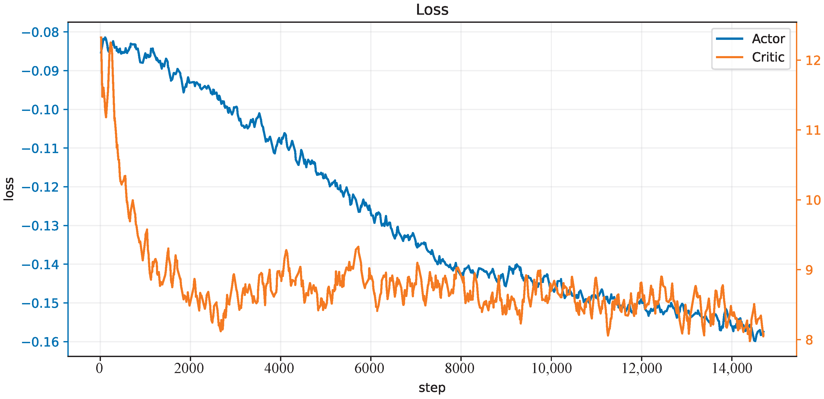
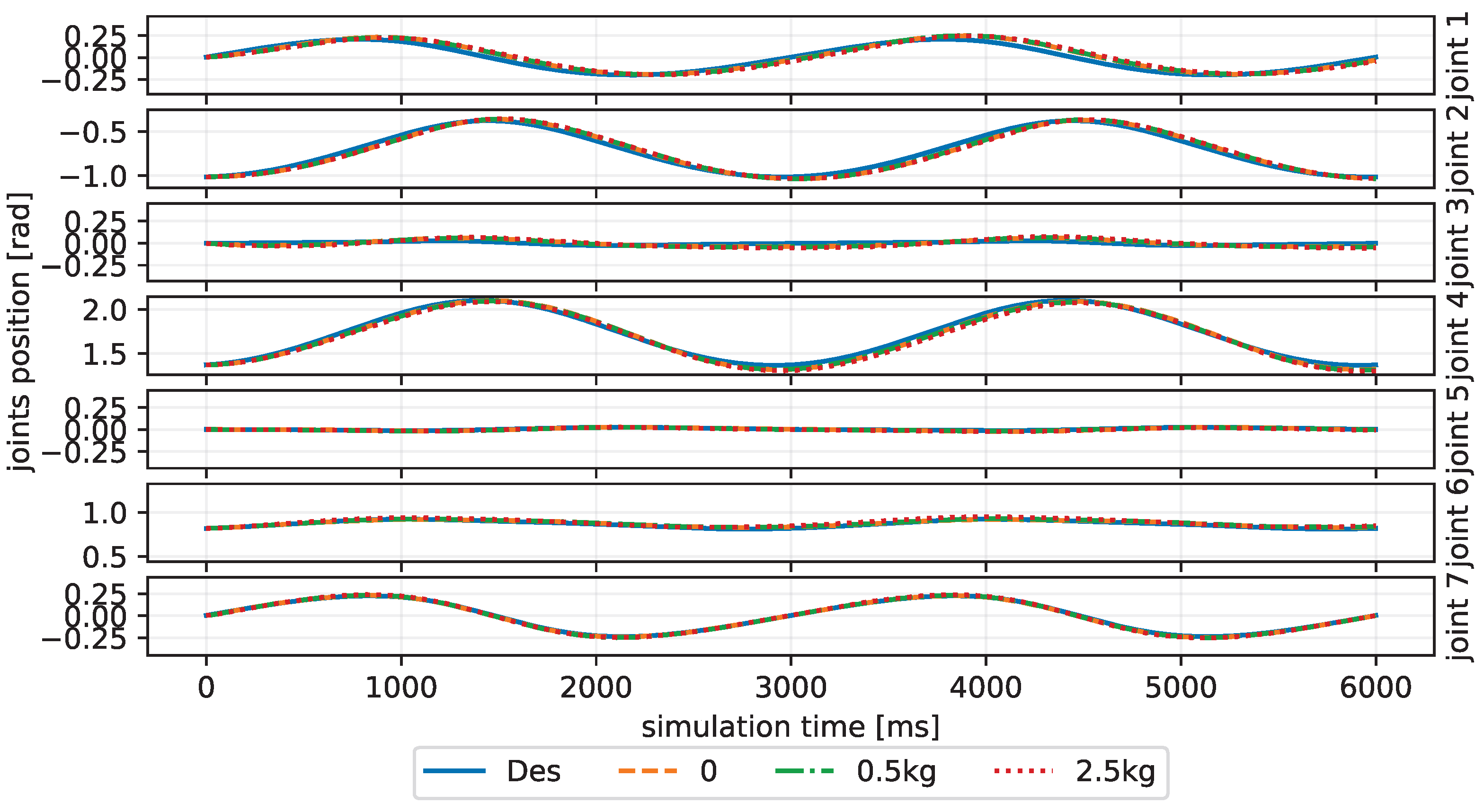
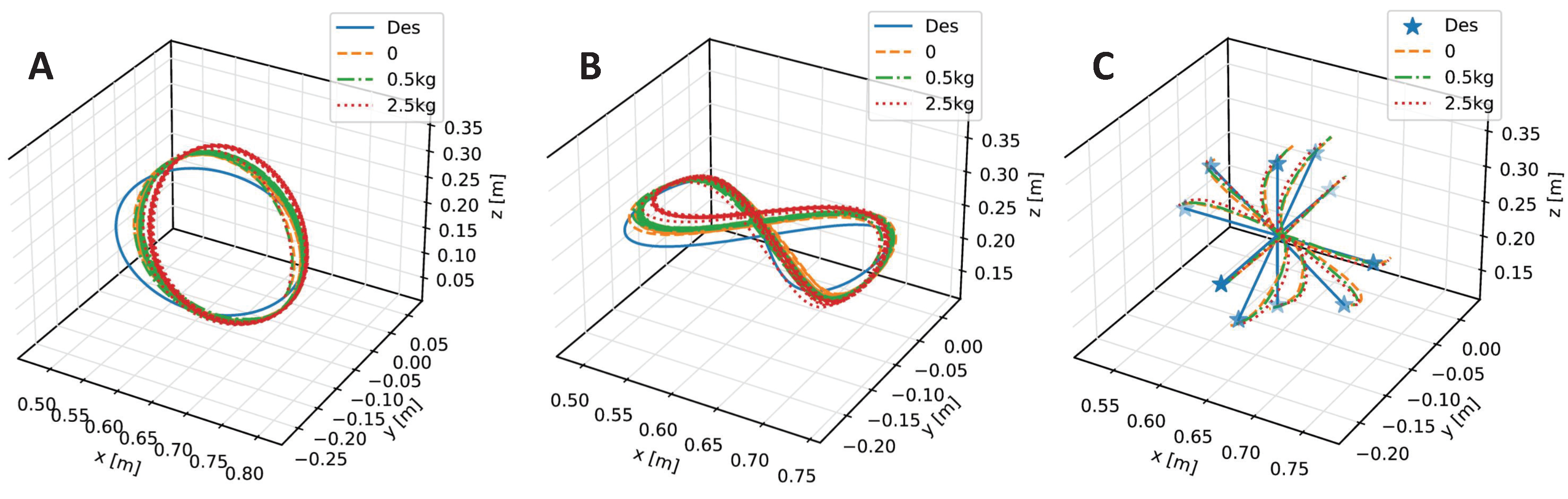
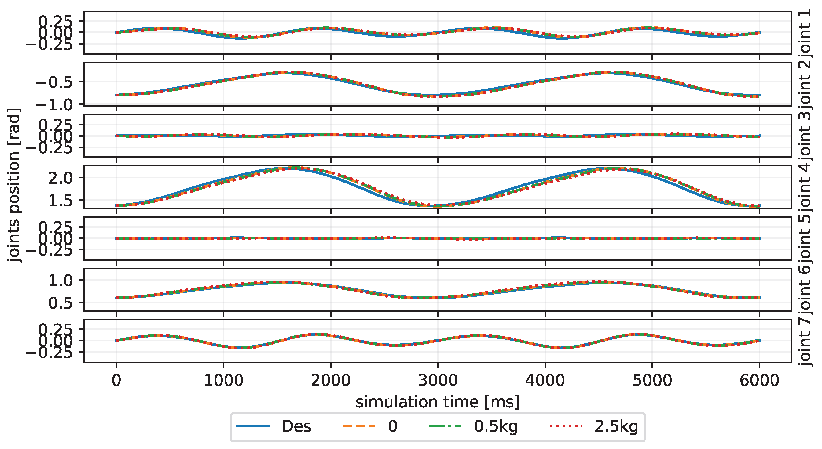
We train our CBMC with a specific trajectory target, which is an inclined circle as described in Equation (
25), and without payload on the end-effector in the PyBullet physics simulator [
38], and 150 trials in each epoch. The initial state of the robot is not on the trajectory at the beginning. One hundred epochs, thus 15 k trials, are performed, and the learning curves of the actor network and critic network are shown in
Figure 4. After this learning process, the controller is applied to different trajectory-tracking tasks and is faced with unknown payloads on the end-effector.
| Algorithm 1 Learning algorithm of CBMC |
- 1:
Load the cerebellum-like SNN - 2:
Initialize main critic network, actor network, target networks, and replay buffer - 3:
Initialize relative frequency F between cerebellum module and CMCM - 4:
for epoch to N do - 5:
Initialize the neurons states - 6:
Initialize the robot states - 7:
Initialize the period reward - 8:
for to M do - 9:
if (t Mod F) == 1 then - 10:
Generate action according to current policy and states - 11:
Update cerebellum-like SNN - 12:
end if - 13:
Calculate torque commands from CBMC - 14:
Execute torque commands and observe new states - 15:
Compute reward f and accumulate the period reward - 16:
if (t Mod F) == 1 and then - 17:
Store transition in replay buffer - 18:
Reset the period reward - 19:
Update the critic and actor networks by training on a small batch of samples from the replay buffer - 20:
Update the target networks - 21:
end if - 22:
end for - 23:
end for
|


