
Application of Machine Learning to Predict COVID-19 Spread via an Optimized BPSO Model


 , ,
, ,  and
and 
Abstract
:1. Introduction
2. Related Work
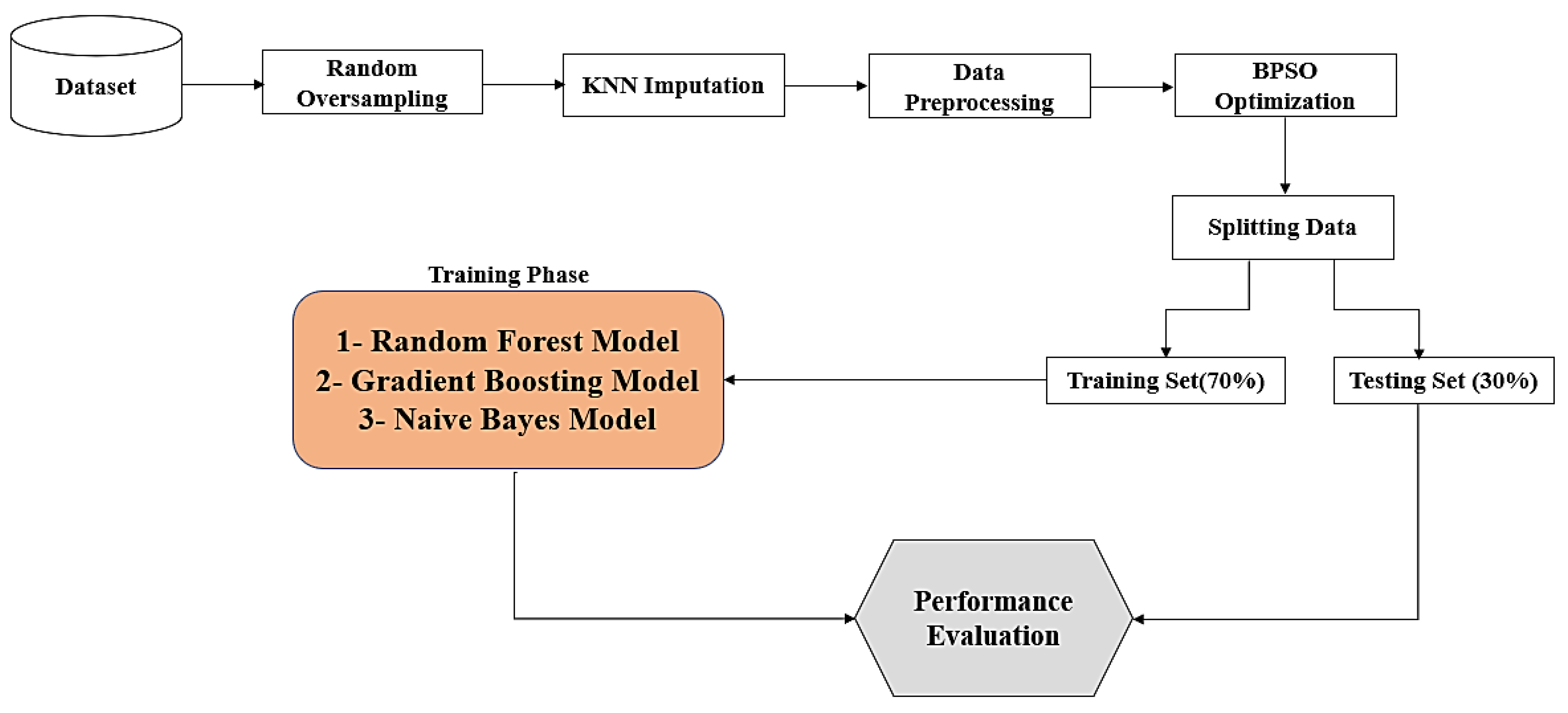
3. Materials and Methods
3.1. Database Collection and Description
3.2. Random Oversampling
3.3. K Nearest Neighbor (KNN) Imputation Algorithm
- Missing completely at random (MCAR): In this case, the dataset contains missing values that are fully independent of any observed variables in the dataset. When data is MCAR, the data analysis performed is unbiased.
- Missing at random (MAR): This means that missing values in the dataset are dependent on observed variables in the dataset. This type of missing data can introduce bias in the analysis, potentially unbalancing the data due to a large number of missing values in one category.
- Missing not at random (MNAR): In this case, missing values in the dataset are dependent on the missing values themselves and do not depend on any other observed variable. Dealing with missing values that are MNAR can be challenging because it is difficult to implement an imputation algorithm that relies on unobserved data.
3.4. Data Preprocessing
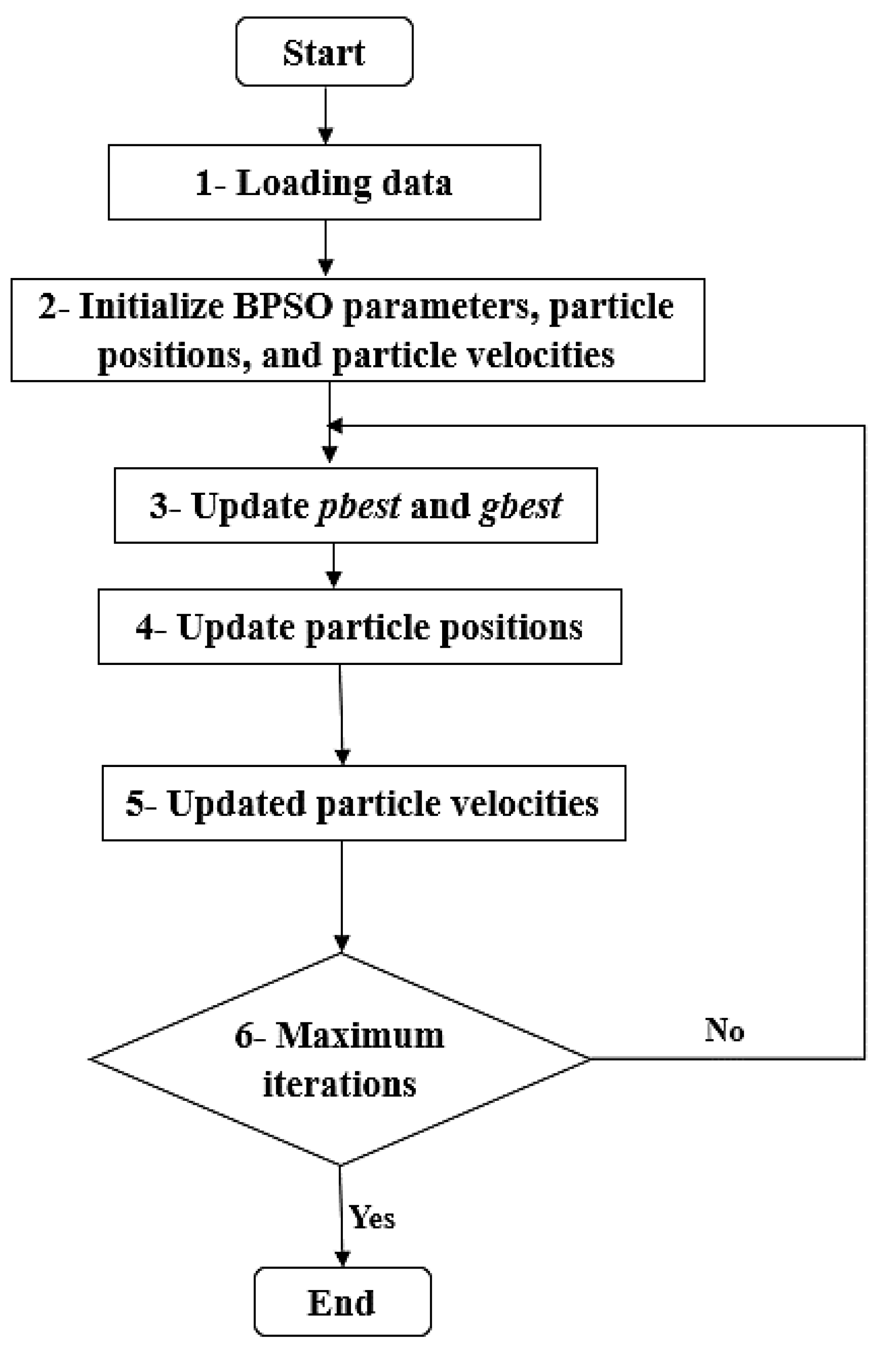
3.5. Particle Swarm Optimization (PSO)
Binary Particle Swarm Optimization (BPSO)
3.6. Machine Learning Models
3.6.1. Random Forest Model
3.6.2. Gradient Boosting Model
3.6.3. Naive Bayes Classifier Model
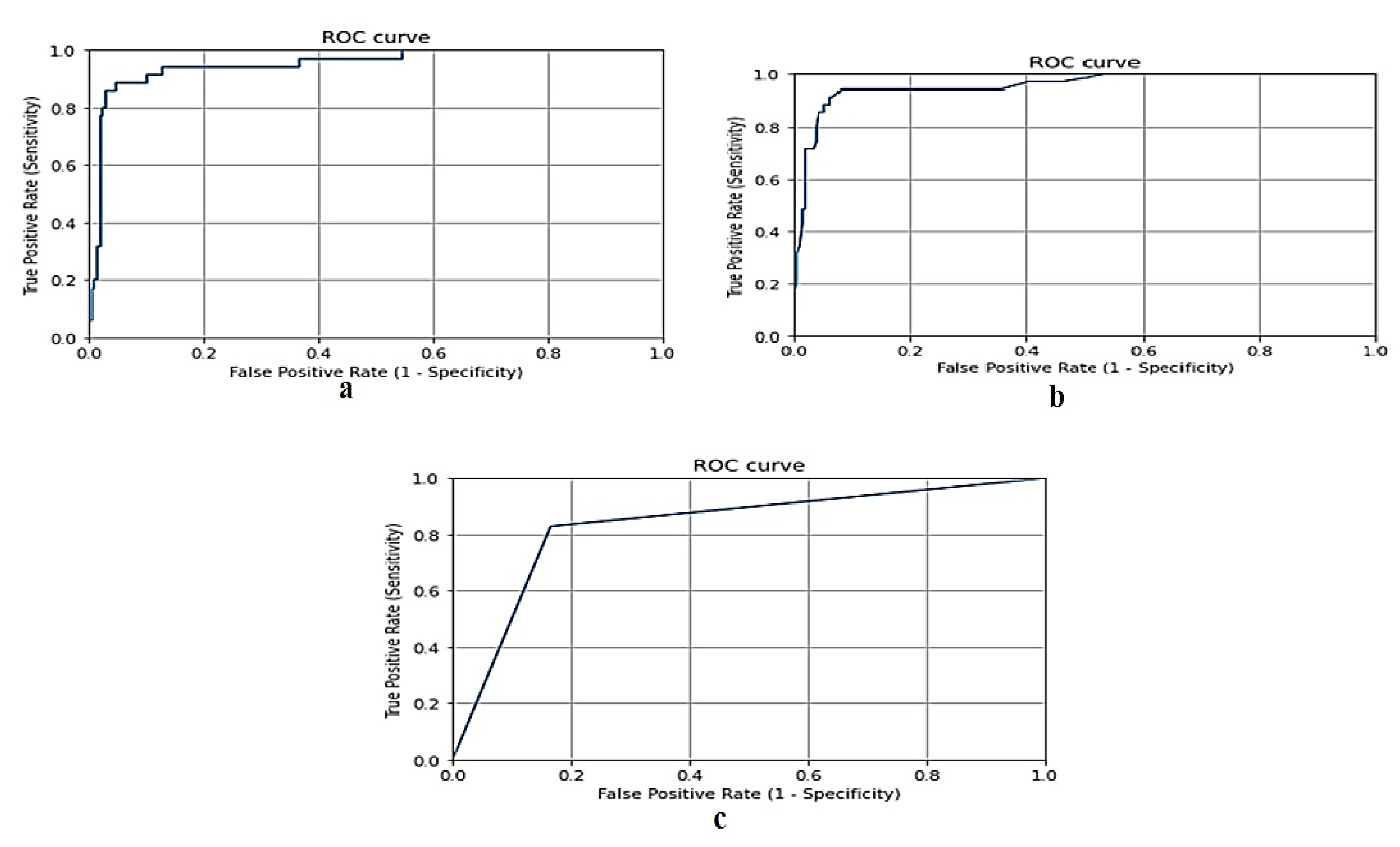
3.7. Evaluation Metrics
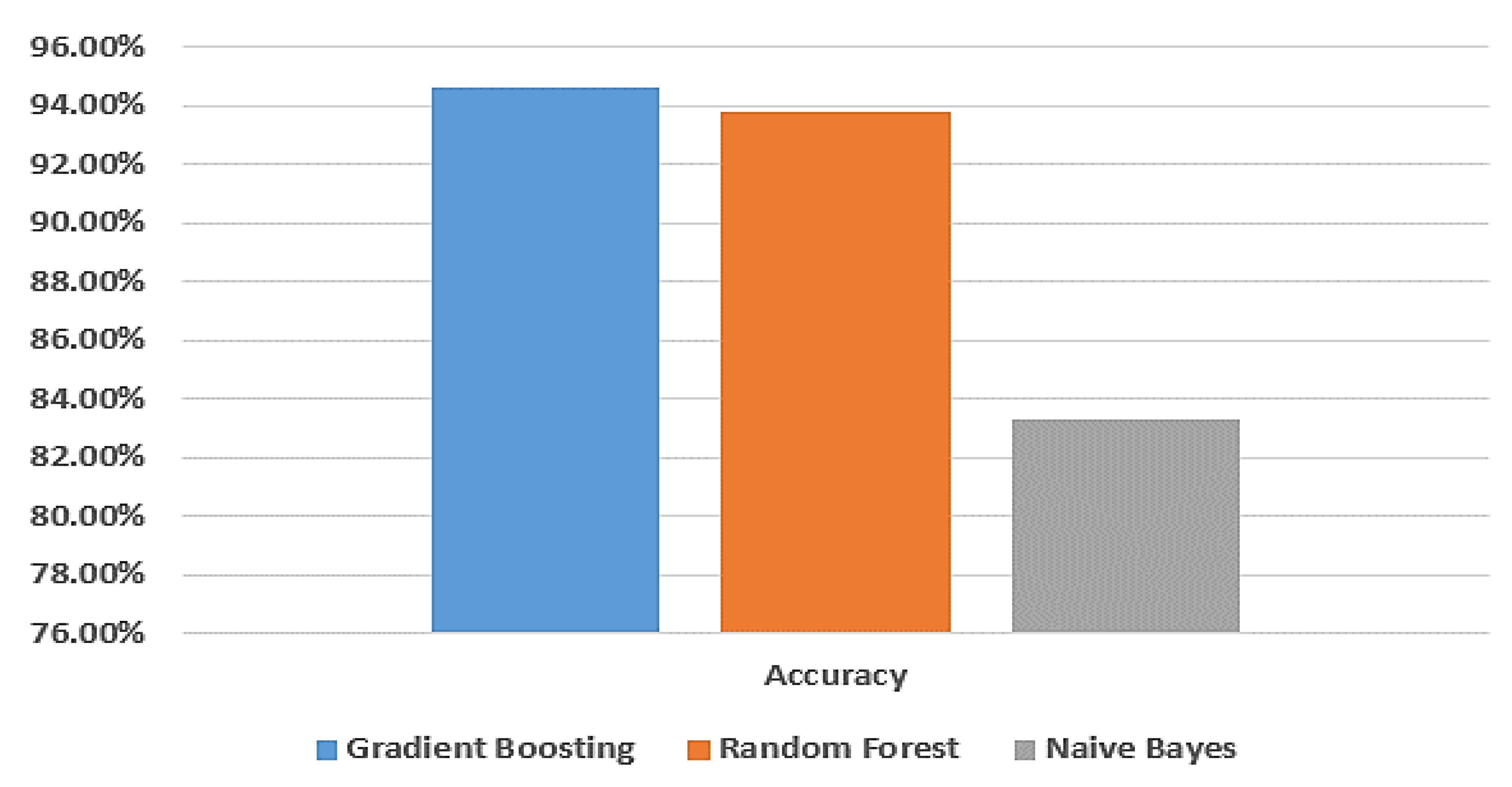
4. Results and Discussion
- Random oversampling was used to balance the data before the training process.
- The KNN imputation algorithm was applied to handle missing data in the dataset.
- Binary Particle Swarm Optimization (BPSO) was utilized as an optimization algorithm to select important features for training, aiming for improved prediction results.
5. Conclusions and Future Work
Author Contributions
Funding
Institutional Review Board Statement
Data Availability Statement
Acknowledgments
Conflicts of Interest
References
- Abdelsalam, M.; Althaqafi, R.M.; Assiri, S.A.; Althagafi, T.M.; Althagafi, S.M.; Fouda, A.Y.; Ramadan, A.; Rabah, M.; Ahmed, R.M.; Ibrahim, Z.S.; et al. Clinical and laboratory findings of COVID-19 in high-altitude inhabitants of Saudi Arabia. Front. Med. 2021, 8, 670195. [Google Scholar] [CrossRef] [PubMed]
- Snuggs, S.; McGregor, S. Food & meal decision making in lockdown: How and who has COVID-19 affected? Food Qual. Prefer. 2021, 89, 104145. [Google Scholar] [PubMed]
- Galanakis, C.M. The food systems in the era of the coronavirus (COVID-19) pandemic crisis. Foods 2020, 9, 523. [Google Scholar] [CrossRef] [PubMed]
- CDC. Novel Coronavirus Reports: Morbidity and Mortality Weekly Report (MMWR); CDC: Atlanta, GA, USA, 2020. [Google Scholar]
- Arias-Reyes, C.; Zubieta-DeUrioste, N.; Poma-Machicao, L.; Aliaga-Raduan, F.; Carvajal-Rodriguez, F.; Dutschmann, M.; Schneider-Gasser, E.M.; Zubieta-Calleja, G.; Soliz, J. Does the pathogenesis of SARS-CoV-2 virus decrease at high-altitude? Respir. Physiol. Neurobiol. 2020, 277, 103443. [Google Scholar] [CrossRef] [PubMed]
- Castagnetto Mizuaray, J.M.; Segovia Juárez, J.L.; Gonzales, G.F. COVID-19 Infections Do Not Change with Increasing Altitudes from 1,000 to 4,700 m. High Alt. Med. Biol. 2020, 21, 428–430. [Google Scholar] [CrossRef] [PubMed]
- Intimayta-Escalante, C.; Rojas-Bolivar, D.; Hancco, I. influence of altitude on the prevalence and case fatality rate of COVID-19 in Peru. High Alt. Med. Biol. 2020, 21, 426–427. [Google Scholar] [CrossRef] [PubMed]
- Lin, E.M.; Goren, A.; Wambier, C. Environmental Effects on Reported Infections and Death Rates of COVID-19 Across 91 Major Brazilian Cities. High Alt. Med. Biol. 2020, 21, 431–433. [Google Scholar] [CrossRef]
- Segovia-Juarez, J.; Castagnetto, J.M.; Gonzales, G.F. High altitude reduces infection rate of COVID-19 but not case-fatality rate. Respir. Physiol. Neurobiol. 2020, 281, 103494. [Google Scholar] [CrossRef]
- Woolcott, O.O.; Bergman, R.N. Mortality attributed to COVID-19 in high-altitude populations. High Alt. Med. Biol. 2020, 21, 409–416. [Google Scholar] [CrossRef]
- Shams, M.Y.; Elzeki, O.M.; Abouelmagd, L.M.; Hassanien, A.E.; Abd Elfattah, M.; Salem, H. HANA: A healthy artificial nutrition analysis model during COVID-19 pandemic. Comput. Biol. Med. 2021, 135, 104606. [Google Scholar] [CrossRef]
- Ferri, M. Why topology for machine learning and knowledge extraction? Mach. Learn. Knowl. Extr. 2019, 1, 115–120. [Google Scholar] [CrossRef]
- De Castro, Y.; Gamboa, F.; Henrion, D.; Hess, R.; Lasserre, J.B. Approximate optimal designs for multivariate polynomial regression. Ann. Stat. 2019, 47, 127–155. [Google Scholar] [CrossRef]
- Hao, Y.; Xu, T.; Hu, H.; Wang, P.; Bai, Y. Prediction and analysis of corona virus disease 2019. PLoS ONE 2020, 15, e0239960. [Google Scholar] [CrossRef] [PubMed]
- Yang, Z.; Zeng, Z.; Wang, K.; Wong, S.S.; Liang, W.; Zanin, M.; Liu, P.; Cao, X.; Gao, Z.; Mai, Z.; et al. Modified SEIR and AI prediction of the epidemics trend of COVID-19 in China under public health interventions. J. Thorac. Dis. 2020, 12, 165. [Google Scholar] [CrossRef] [PubMed]
- Adnan, M.; Altalhi, M.; Alarood, A.A.; Uddin, M.I. Modeling the Spread of COVID-19 by Leveraging Machine and Deep Learning Models. Intell. Autom. Soft Comput. 2022, 31, 1857–1872. [Google Scholar] [CrossRef]
- Batista, A.; Miraglia, J.; Donato, T.; Chiavegatto, F.A. COVID-19 diagnosis prediction in emergency care patients: A machine learning approach. medRxiv 2020. [Google Scholar] [CrossRef]
- Sun, L.; Song, F.; Shi, N.; Liu, F.; Li, S.; Li, P.; Zhang, W.; Jiang, X.; Zhang, Y.; Sun, L.; et al. Combination of four clinical indicators predicts the severe/critical symptom of patients infected COVID-19. J. Clin. Virol. 2020, 128, 104431. [Google Scholar] [CrossRef]
- Salama, A.; Darwsih, A.; Hassanien, A.E. Artificial intelligence approach to predict the COVID-19 patient’s recovery. In Digital Transformation and Emerging Technologies for Fighting COVID-19 Pandemic: Innovative Approaches; Springer: Cham, Switzerland, 2021; pp. 121–133. [Google Scholar]
- Laatifi, M.; Douzi, S.; Bouklouz, A.; Ezzine, H.; Jaafari, J.; Zaid, Y.; El Ouahidi, B.; Naciri, M. Machine learning approaches in COVID-19 severity risk prediction in Morocco. J. Big Data 2022, 9, 5. [Google Scholar] [CrossRef]
- Banoei, M.M.; Dinparastisaleh, R.; Zadeh, A.V.; Mirsaeidi, M. Machine-learning-based COVID-19 mortality prediction model and identification of patients at low and high risk of dying. Crit. Care 2021, 25, 328. [Google Scholar] [CrossRef]
- Iwendi, C.; Bashir, A.K.; Peshkar, A.; Sujatha, R.; Chatterjee, J.M.; Pasupuleti, S.; Mishra, R.; Pillai, S.; Jo, O. COVID-19 patient health prediction using boosted random forest algorithm. Front. Public Health 2020, 8, 357. [Google Scholar] [CrossRef]
- JHU CSSE. Novel Coronavirus (COVID-19) Cases Data; Johns Hopkins University Center for Systems Science and Engineering (JHU CCSE): Baltimore, MD, USA, 2020. [Google Scholar]
- Pourhomayoun, M.; Shakibi, M. Predicting mortality risk in patients with COVID-19 using machine learning to help medical decision-making. Smart Health 2021, 20, 100178. [Google Scholar] [CrossRef] [PubMed]
- Yadaw, A.S.; Li, Y.C.; Bose, S.; Iyengar, R.; Bunyavanich, S.; Pandey, G. Clinical predictors of COVID-19 mortality. medRxiv 2020. [Google Scholar] [CrossRef]
- Moulaei, K.; Shanbehzadeh, M.; Mohammadi-Taghiabad, Z.; Kazemi-Arpanahi, H. Comparing machine learning algorithms for predicting COVID-19 mortality. BMC Med. Inform. Decis. Mak. 2022, 22, 2. [Google Scholar] [CrossRef] [PubMed]
- Hu, C.; Liu, Z.; Jiang, Y.; Shi, O.; Zhang, X.; Xu, K.; Suo, C.; Wang, Q.; Song, Y.; Yu, K.; et al. Early prediction of mortality risk among patients with severe COVID-19, using machine learning. Int. J. Epidemiol. 2020, 49, 1918–1929. [Google Scholar] [CrossRef] [PubMed]
- Chae, S.; Kwon, S.; Lee, D. Predicting infectious disease using deep learning and big data. Int. J. Environ. Res. Public Health 2018, 15, 1596. [Google Scholar] [CrossRef]
- Ezzat, D.; Ella, H.A. GSA-DenseNet121-COVID-19: A hybrid deep learning architecture for the diagnosis of COVID-19 disease based on gravitational search optimization algorithm. arXiv 2020, arXiv:2004.05084. [Google Scholar]
- Yang, Y.; Yang, M.; Shen, C.; Wang, F.; Yuan, J.; Li, J.; Zhang, M.; Wang, Z.; Xing, L.; Wei, J.; et al. Evaluating the accuracy of different respiratory specimens in the laboratory diagnosis and monitoring the viral shedding of 2019-nCoV infections. medRxiv 2020. [Google Scholar]
- Hayaty, M.; Muthmainah, S.; Ghufran, S.M. Random and synthetic over-sampling approach to resolve data imbalance in classification. Int. J. Artif. Intell. Res. 2020, 4, 86–94. [Google Scholar] [CrossRef]
- Brennan, P. A Comprehensive Survey of Methods for Overcoming the Class Imbalance Problem in Fraud Detection; Institute of technology Blanchardstown: Dublin, Ireland, 2012. [Google Scholar]
- Huang, J.; Keung, J.W.; Sarro, F.; Li, Y.F.; Yu, Y.T.; Chan, W.K.; Sun, H. Cross-validation based K nearest neighbor imputation for software quality datasets: An empirical study. J. Syst. Softw. 2017, 132, 226–252. [Google Scholar] [CrossRef]
- Malarvizhi, R.; Thanamani, A.S. K-nearest neighbor in missing data imputation. Int. J. Eng. Res. Dev. 2012, 5, 5–7. [Google Scholar]
- Alkhammash, E.H.; Hadjouni, M.; Elshewey, A.M. A Hybrid Ensemble Stacking Model for Gender Voice Recognition Approach. Electronics 2022, 11, 1750. [Google Scholar] [CrossRef]
- García, S.; Luengo, J.; Herrera, F. Data Preprocessing in Data Mining; Springer International Publishing: Cham, Switzerland, 2015. [Google Scholar]
- Rodríguez, C.K. A Computational Environment for Data Preprocessing in Supervised Classification; University of Puerto Rico, Mayaguez: San Juan, Puerto Rico, 2004. [Google Scholar]
- Li, A.D.; Xue, B.; Zhang, M. Improved binary particle swarm optimization for feature selection with new initialization and search space reduction strategies. Appl. Soft Comput. 2021, 106, 107302. [Google Scholar] [CrossRef]
- Too, J.; Abdullah, A.R.; Mohd Saad, N. A new co-evolution binary particle swarm optimization with multiple inertia weight strategy for feature selection. Informatics 2019, 6, 21. [Google Scholar] [CrossRef]
- Cervante, L.; Xue, B.; Zhang, M.; Shang, L. Binary particle swarm optimisation for feature selection: A filter based approach. In Proceedings of the 2012 IEEE Congress on Evolutionary Computation, Brisbane, Australia, 10–15 June 2012; pp. 1–8. [Google Scholar]
- Nguyen, B.H.; Xue, B.; Andreae, P.; Zhang, M. A new binary particle swarm optimization approach: Momentum and dynamic balance between exploration and exploitation. IEEE Trans. Cybern. 2019, 51, 589–603. [Google Scholar] [CrossRef] [PubMed]
- Tarek, Z.; Elshewey, A.M.; Shohieb, S.M.; Elhady, A.M.; El-Attar, N.E.; Elseuofi, S.; Shams, M.Y. Soil Erosion Status Prediction Using a Novel Random Forest Model Optimized by Random Search Method. Sustainability 2023, 15, 7114. [Google Scholar] [CrossRef]
- Shams, M.Y.; El-kenawy, E.S.; Ibrahim, A.; Elshewey, A.M. A hybrid dipper throated optimization algorithm and particle swarm optimization (DTPSO) model for hepatocellular carcinoma (HCC) prediction. Biomed. Signal Process. Control. 2023, 85, 104908. [Google Scholar] [CrossRef]
- Natekin, A.; Knoll, A. Gradient boosting machines, a tutorial. Front. Neurol. 2013, 7, 21. [Google Scholar] [CrossRef]
- Konstantinov, A.; Utkin, L.; Muliukha, V. Gradient boosting machine with partially randomized decision trees. In Proceedings of the 2021 28th Conference of Open Innovations Association (FRUCT), Moscow, Russia, 27–29 January 2021; pp. 167–173. [Google Scholar]
- Elshewey, A.M.; Shams, M.Y.; El-Rashidy, N.; Elhady, A.M.; Shohieb, S.M.; Tarek, Z. Bayesian optimization with support vector machine model for parkinson disease classification. Sensors 2023, 23, 2085. [Google Scholar] [CrossRef]
- Berrar, D. Bayes’ theorem and naive Bayes classifier. Encycl. Bioinform. Comput. Biol. ABC Bioinform. 2018, 403, 412. [Google Scholar]
- Zhang, H.; Li, D. Naïve Bayes text classifier. In Proceedings of the 2007 IEEE International Conference on Granular Computing (GRC 2007), San Jose, CA, USA, 2–4 November 2007; p. 708. [Google Scholar]
- Fouad, Y.; Osman, A.M.; Hassan, S.A.; El-Bakry, H.M.; Elshewey, A.M. Adaptive Visual Sentiment Prediction Model Based on Event Concepts and Object Detection Techniques in Social Media. Int. J. Adv. Comput. Sci. Appl. 2023, 14, 252–256. [Google Scholar] [CrossRef]
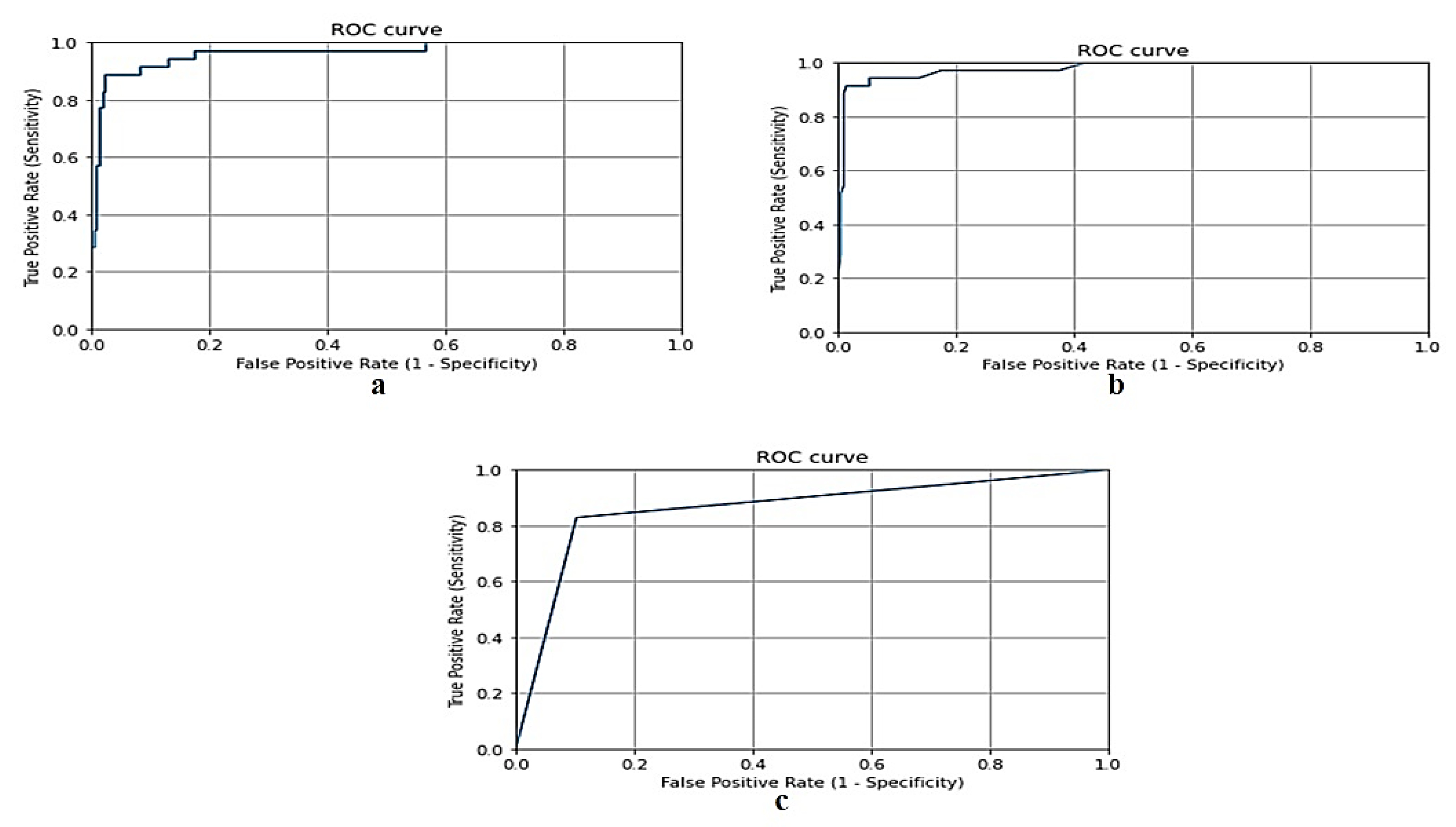
- Hoo, Z.H.; Candlish, J.; Teare, D. What is an ROC curve? Emerg. Med. J. 2017, 34, 357–359. [Google Scholar] [CrossRef]

| Sociodemographic Data and Comorbidities | Possible Infection Source | ||||
|---|---|---|---|---|---|
| Mean age | 39.4 | ±15.9 | Known history of positive contact | 378 | 32.7% |
| Male patients (n) | 788 | 63.3% | Health care worker | 127 | 11.3% |
| Female patients (n) | 456 | 36.7% | Laboratory investigations | ||
| Taif city patients (n) | 1036 | 83.3% | Mean Red blood cell count (RBCs) | 7.2 | ±2.09 |
| Jeddah city patients (n) | 208 | 16.7% | Mean Hemoglobin | 15.6 | ±6.99 |
| Positive COVID-19 PCR results | 1013 | 81.5% | Mean Hematocrit | 46.5 | ±15.63 |
| Negative COVID-19 PCR results | 230 | 18.5% | Mean MCV | 82.8 | ±38.81 |
| Diabetes mellites | 228 | 18.4% | Mean MCH | 28.5 | ±8.67 |
| Hypertension | 184 | 14.8% | Mean MCHC | 31.9 | ±10.48 |
| Asthma | 46 | 3.7% | Mean RDW (%) | 29.4 | ±66.87 |
| Deep venous thrombosis (DVT) | 7 | 0.6% | Mean Platelet Count | 250.9 | ±94.23 |
| Pulmonary embolism (PE) | 10 | 0.8% | Mean Total WBCs | 10.92 | ±13.46 |
| Myocardial infarction (MI) | 13 | 1% | Mean Neutrophil | 51.56 | ±22.04 |
| Ischemic stroke | 20 | 1.6% | Mean Lymphocyte | 27.70 | ±16.64 |
| Acute respiratory distress syndrome (ARDS) | 25 | 2% | Mean basophil | 3.07 | ±9.75 |
| Acute large vessel occlusion | 3 | 0.2% | Mean Eosinophil | 2.12 | ±3.00 |
| Coronary disease | 29 | 2.3% | Mean Monocyte | 7.32 | ±6.05 |
| Tumors | 9 | 0.7% | Mean INR | 4.51 | ±9.04 |
| Chronic kidney disease | 26 | 2.1% | Mean PT | 16.32 | ±10.11 |
| Hospital course | Mean aPTT | 26.36 | ±13.62 | ||
| Mean days of hospitalization | 6.25 | ±6.25 | Mean D-dimer | 10.07 | ±123.48 |
| Patient was admitted to the intensive care unit | 273 | 23.1% | Mean ESR | 28.4 | ±176.27 |
| Discharged due to recovery | 1009 | 81.2% | Mean CRP | 49.8 | ±144.4 |
| Discharged due to death | 45 | 4.2% | Mean Ferritin | 269.1 | ±359.69 |
| Discharged upon the patients’ request (DAMA) | 25 | 2.3% | Mean ALT | 47.9 | ±111.75 |
| Presenting symptoms | Mean AST | 30.6 | ±28.31 | ||
| Fever | 794 | 68.2% | Mean ALP | 66.4 | ±54.2 |
| Cough | 646 | 52% | Mean Albumin | 30.9 | ±18.06 |
| Shortness of Breath | 575 | 49.4% | Mean Bilirubin | 6.35 | ±8.03 |
| GIT symptoms | 312 | 26.8% | Mean Serum Creatinine test | 36.18 | ±53.62 |
| Headache, sore throat, or rhinorrhea | 259 | 22.6% | Mean Blood urea nitrogen (BUN) | 14.28 | ±22.38 |
| Smell loss | 201 | 20% | Mean troponin T | 9.70 | ±12.70 |
| Models | Accuracy | Training Score | Testing Score | F-Measure | Recall | Precision |
|---|---|---|---|---|---|---|
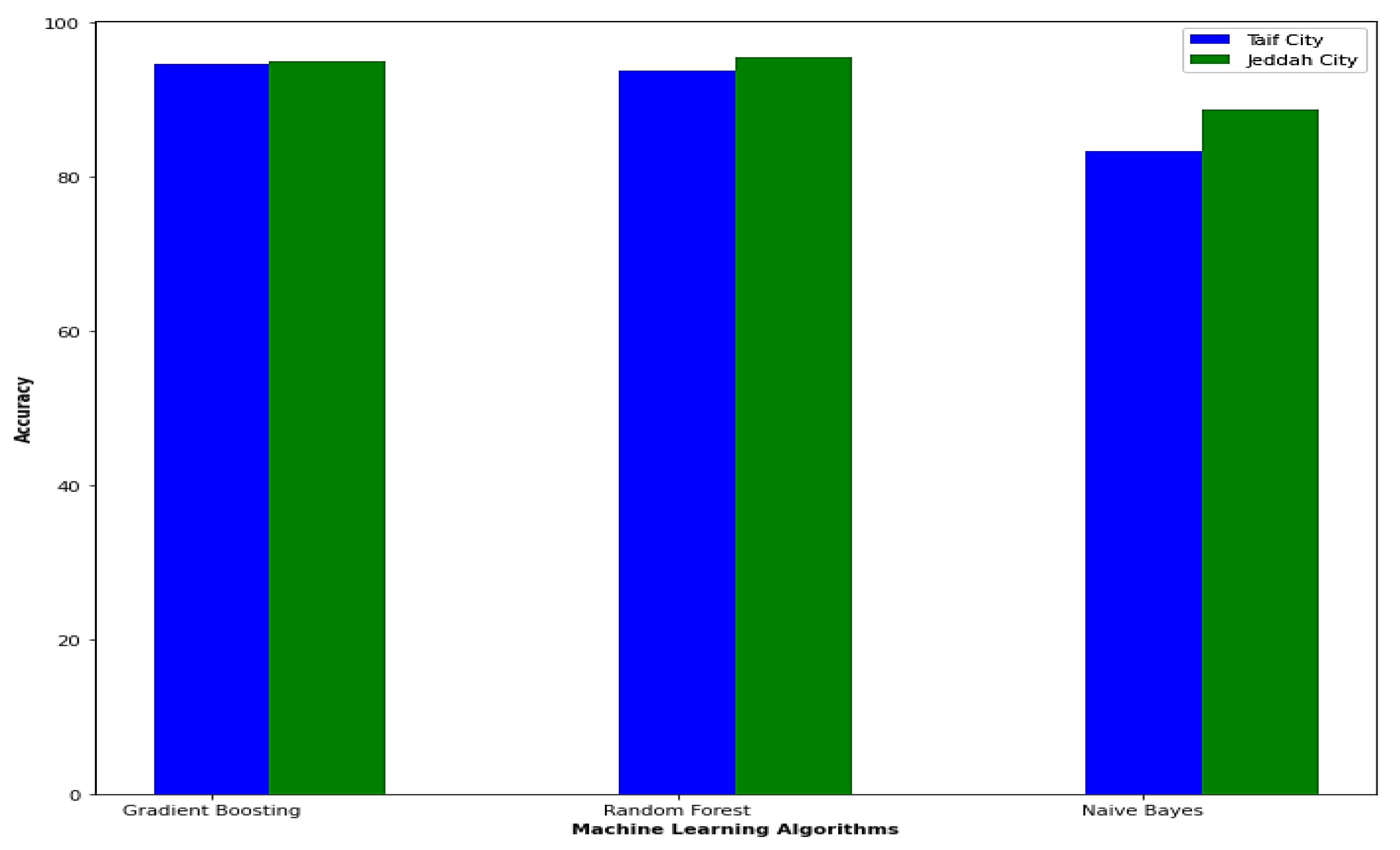
| Gradient Boosting | 94.6% | 100% | 94.5% | 94.5% | 94.6% | 94.6% |
| Random Forest | 93.8% | 100% | 93.7% | 93.6% | 93.7% | 93.7% |
| Naive Bayes | 83.3% | 87.7% | 83.4% | 83.3% | 83.3% | 83.3% |
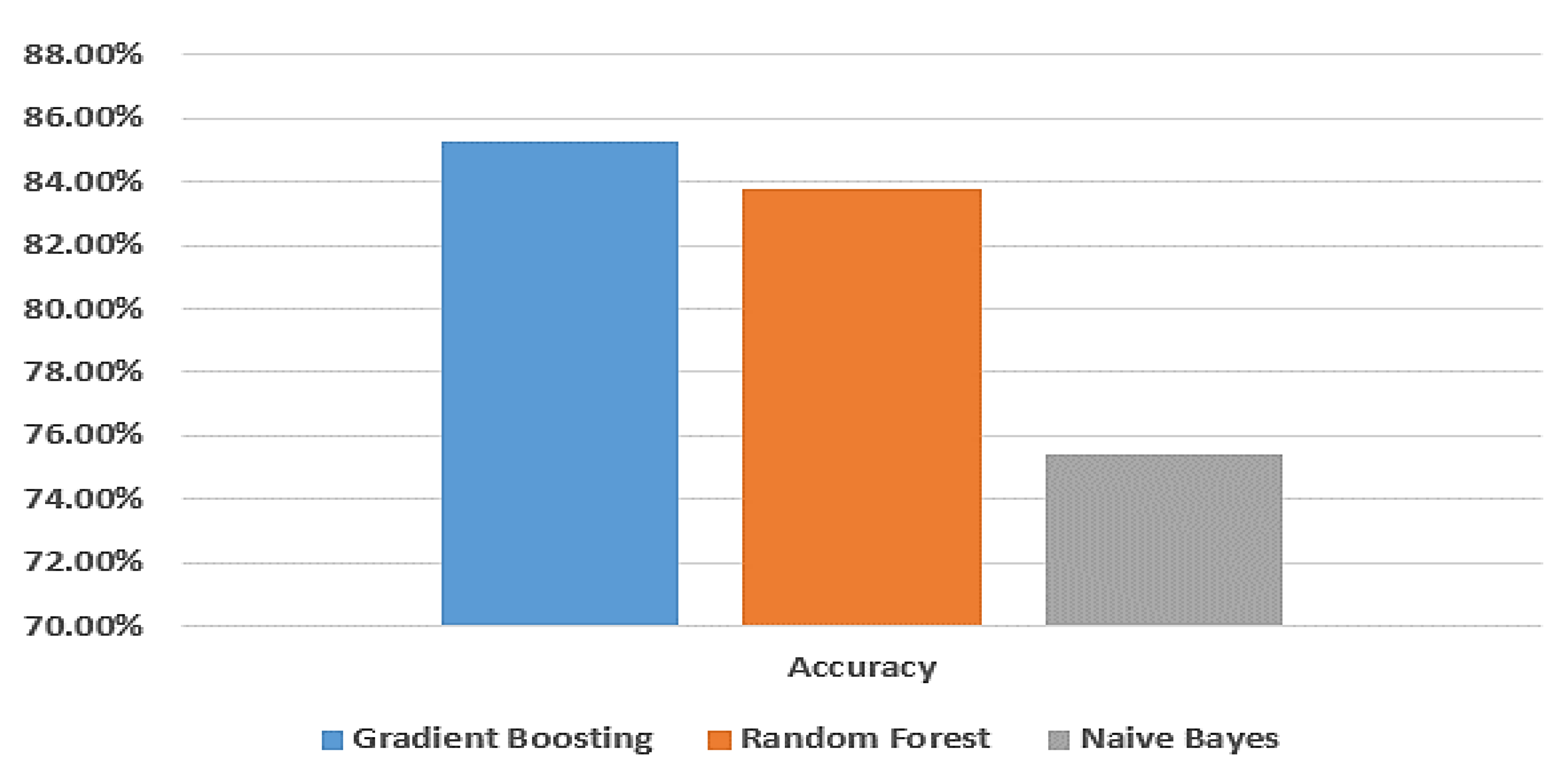
| Models | Accuracy | Training Score | Testing Score | F-Measure | Recall | Precision |
|---|---|---|---|---|---|---|
| Gradient Boosting | 85.3% | 95.2% | 85.4% | 85.2% | 85.6% | 85.6% |
| Random Forest | 83.8% | 94.7% | 83.7% | 83.5% | 83.8% | 83.8% |
| Naive Bayes | 75.4% | 80.3% | 75.3% | 75.6% | 75.6% | 75.6% |
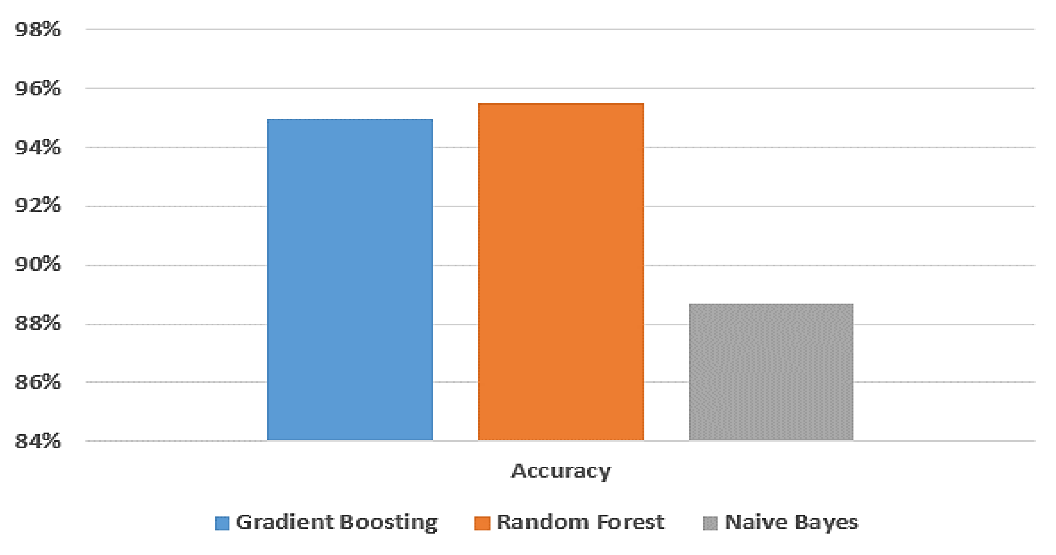
| Models | Accuracy | Training Score | Testing Score | F-Measure | Recall | Precision |
|---|---|---|---|---|---|---|
| Gradient Boosting | 95% | 100% | 95.1% | 95% | 95% | 95% |
| Random Forest | 95.5% | 100% | 95.4% | 95.5% | 95.5% | 95.5% |
| Naive Bayes | 88.7% | 88.4% | 88.1% | 88.7% | 88.6% | 88.6% |
| Studies | Model | Accuracy |
|---|---|---|
| Ref [19] | SVM | 85% |
| Ref [24] | ANN | 89.98% |
| Ref [26] | RF | 95.03% |
| Proposed Work for high-altitude area | BPSO with gradient boosting | 94.6% |
| Proposed Work for sea-level area | BPSO with random forest | 95.5% |
| Model | Accuracy |
|---|---|
| BPSO | 95.5% |
| GA | 91.3% |
| SA | 90.6% |
| DE | 90.4% |
Disclaimer/Publisher’s Note: The statements, opinions and data contained in all publications are solely those of the individual author(s) and contributor(s) and not of MDPI and/or the editor(s). MDPI and/or the editor(s) disclaim responsibility for any injury to people or property resulting from any ideas, methods, instructions or products referred to in the content. |
© 2023 by the authors. Licensee MDPI, Basel, Switzerland. This article is an open access article distributed under the terms and conditions of the Creative Commons Attribution (CC BY) license (https://creativecommons.org/licenses/by/4.0/).
Share and Cite
Alkhammash, E.H.; Assiri, S.A.; Nemenqani, D.M.; Althaqafi, R.M.M.; Hadjouni, M.; Saeed, F.; Elshewey, A.M. Application of Machine Learning to Predict COVID-19 Spread via an Optimized BPSO Model. Biomimetics 2023, 8, 457. https://doi.org/10.3390/biomimetics8060457
Alkhammash EH, Assiri SA, Nemenqani DM, Althaqafi RMM, Hadjouni M, Saeed F, Elshewey AM. Application of Machine Learning to Predict COVID-19 Spread via an Optimized BPSO Model. Biomimetics. 2023; 8(6):457. https://doi.org/10.3390/biomimetics8060457
Chicago/Turabian StyleAlkhammash, Eman H., Sara Ahmad Assiri, Dalal M. Nemenqani, Raad M. M. Althaqafi, Myriam Hadjouni, Faisal Saeed, and Ahmed M. Elshewey. 2023. "Application of Machine Learning to Predict COVID-19 Spread via an Optimized BPSO Model" Biomimetics 8, no. 6: 457. https://doi.org/10.3390/biomimetics8060457
APA StyleAlkhammash, E. H., Assiri, S. A., Nemenqani, D. M., Althaqafi, R. M. M., Hadjouni, M., Saeed, F., & Elshewey, A. M. (2023). Application of Machine Learning to Predict COVID-19 Spread via an Optimized BPSO Model. Biomimetics, 8(6), 457. https://doi.org/10.3390/biomimetics8060457