
Effects of Different Motion Parameters on the Interaction of Fish School Subsystems

Abstract
:1. Introduction
2. Methods
2.1. Fluid Systems—The Lattice Boltzmann Method
2.2. Non-Iterative IBM of the Fluid Interactions with Fish Bodies
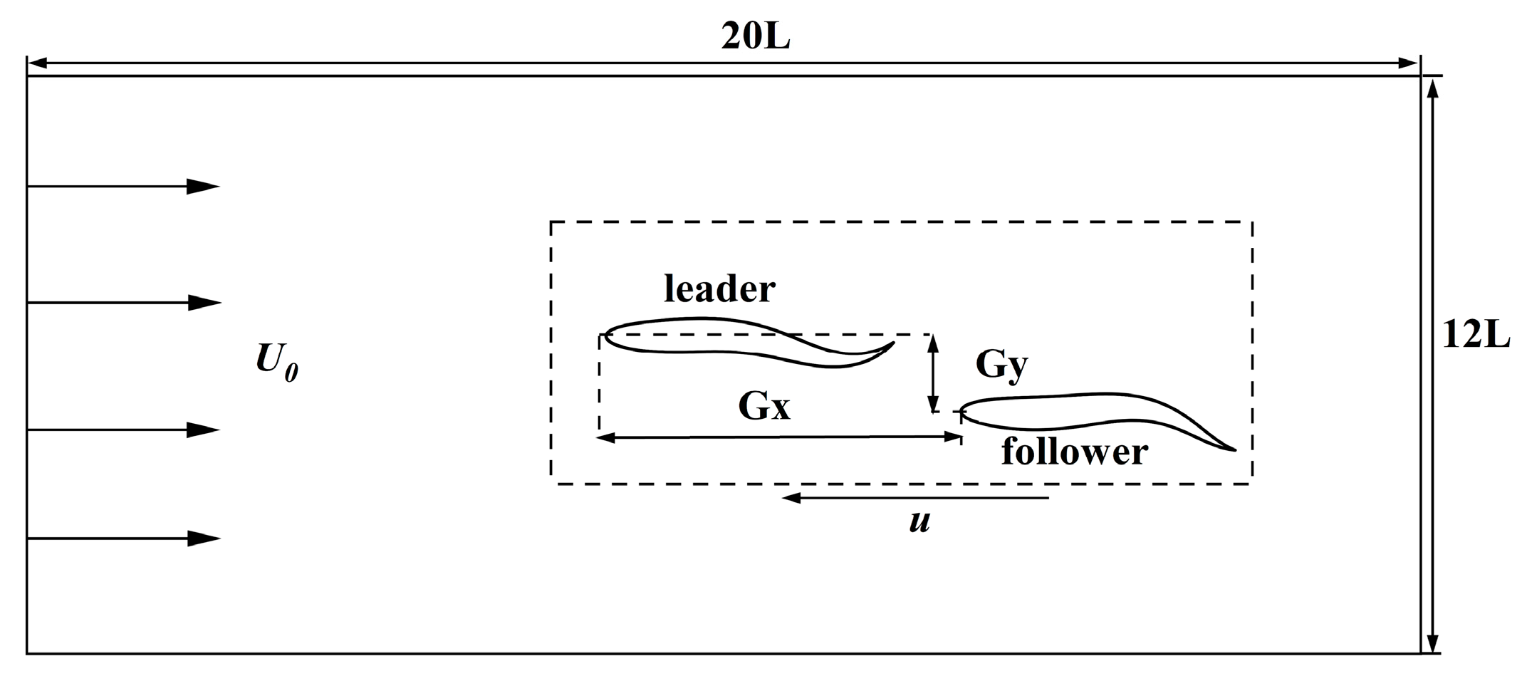
2.3. Configuration Scheme
2.4. Performance Parameters
3. Results
3.1. Verification of the Fluid–Structure Coupling System
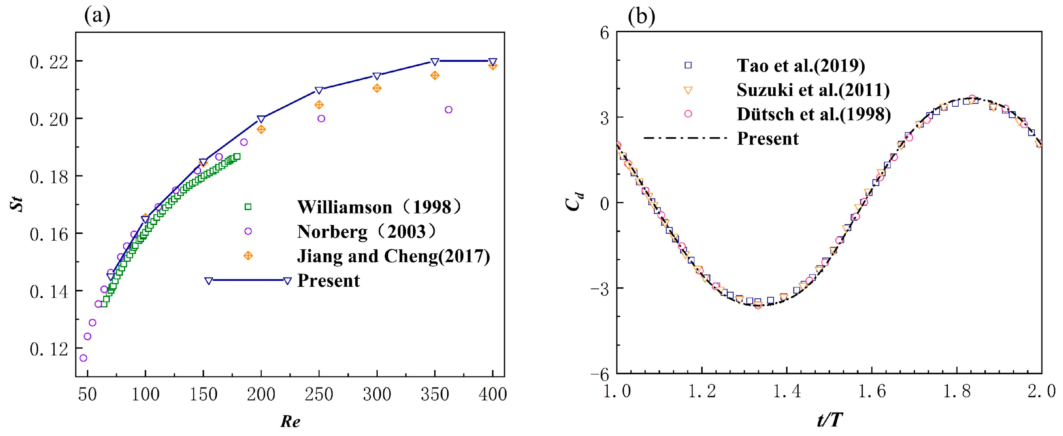
3.1.1. Cylinder Fixed in a Uniform Incoming Flow

| Re | 40 | 100 | 200 | |||
|---|---|---|---|---|---|---|
| ΔCL | ΔCL | ΔCL | ||||
| Present | 1.582 | - | 1.345 | 0.67 | 1.339 | 1.41 |
| Linnick [46] | 1.61 | - | 1.38 | 0.674 | 1.37 | 1.40 |
| Liu et al. [47] | - | - | 1.35 | 0.678 | 1.31 | 1.38 |
| Rosis [48] | 1.50–1.71 | - | 1.28–1.46 | 0.56–0.78 | 1.31–1.45 | 1.20–1.56 |
| Russell [49] | 1.60 | - | 1.43 | 0.644 | 1.45 | 1.26 |
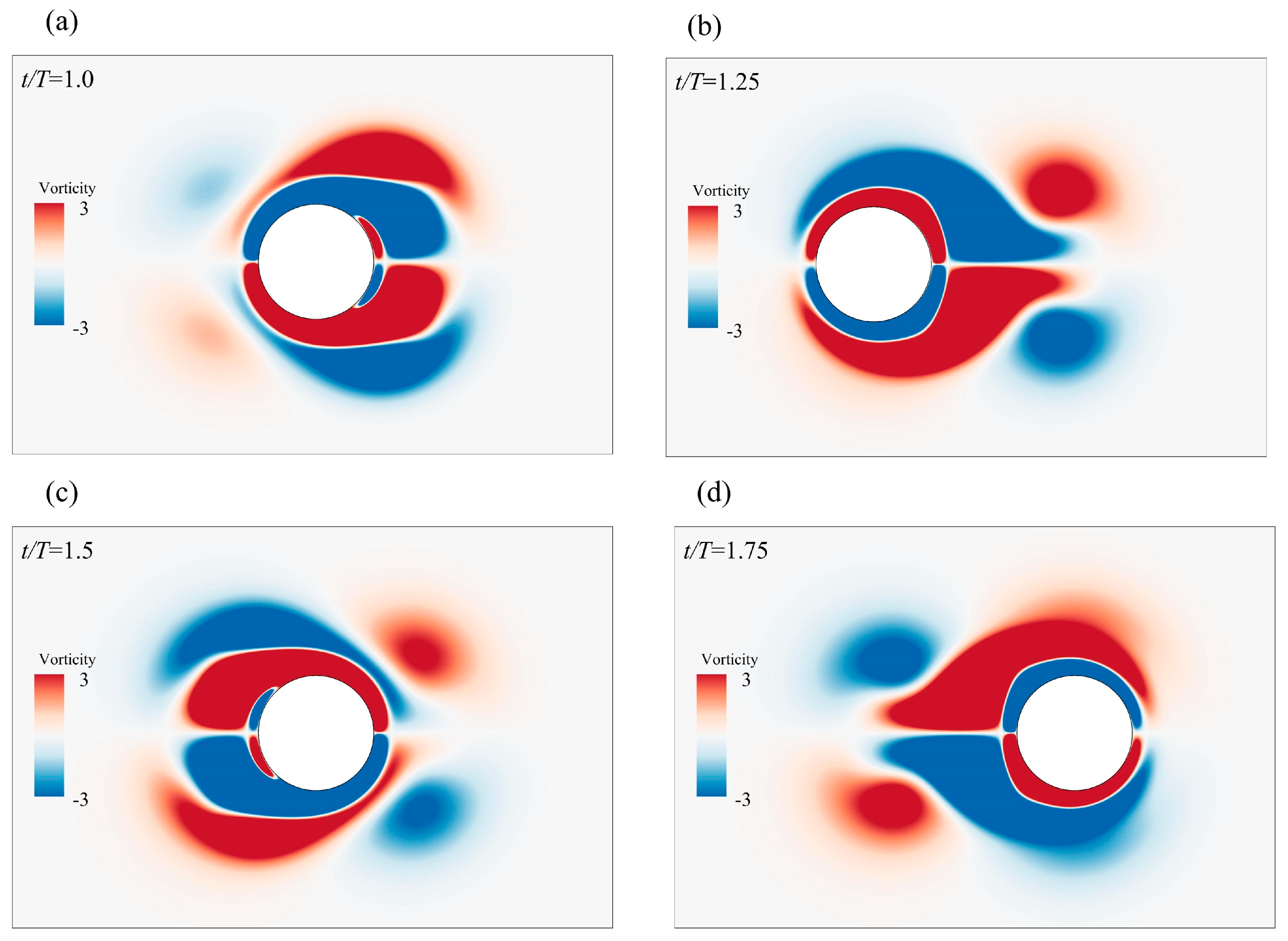
3.1.2. Simulating a Cylinder Oscillating in a Stationary Fluid
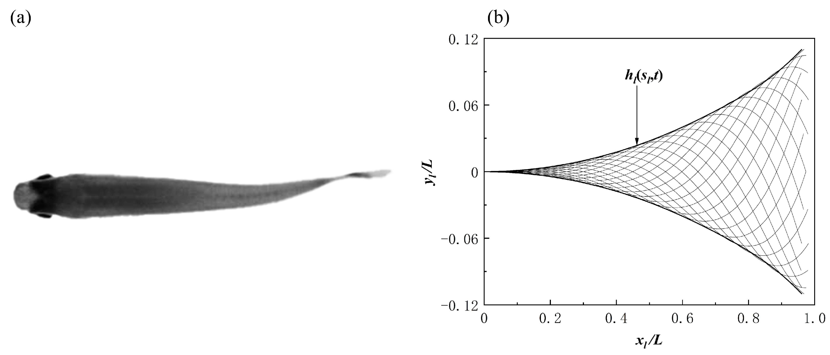
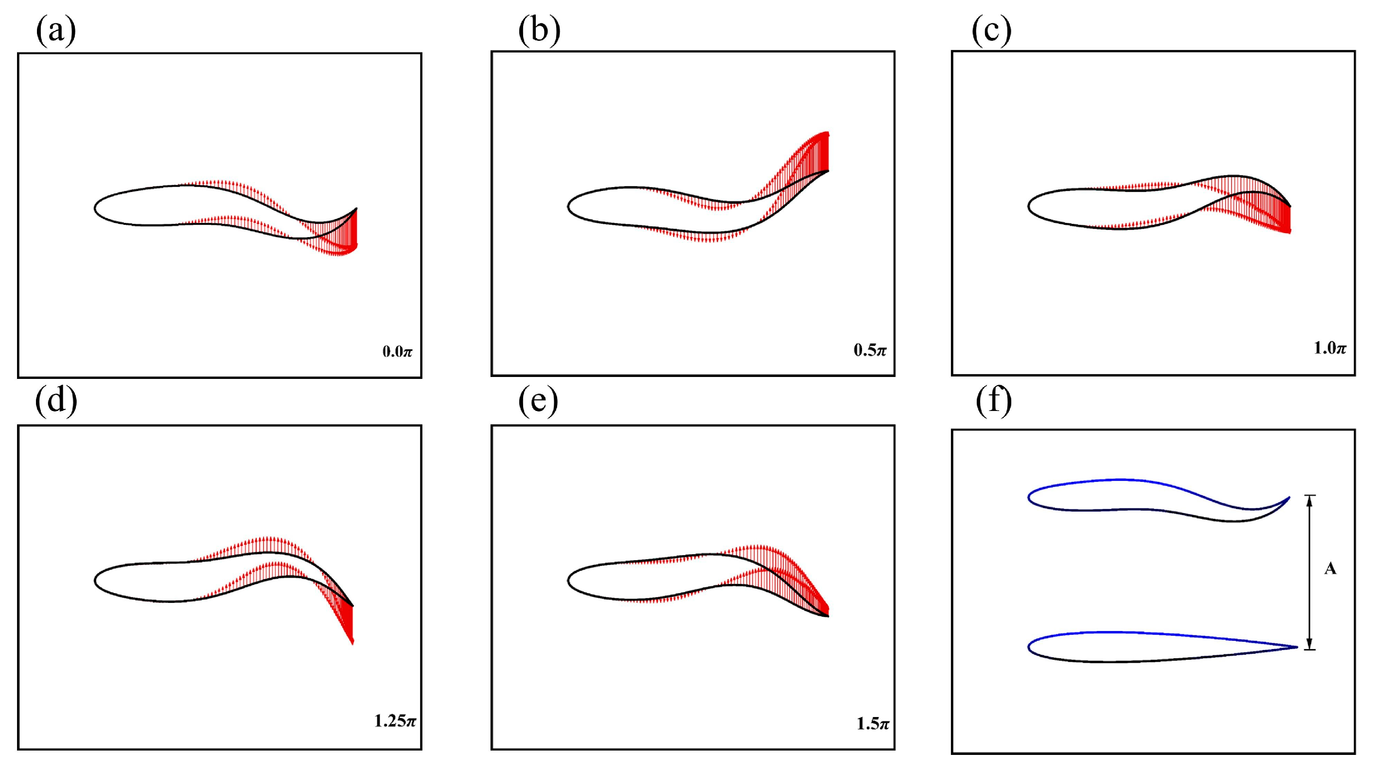
3.1.3. Simulation of the Autonomous Propulsion of Anguilliform Swimmers in Stationary Fluids
3.2. Simulation Results
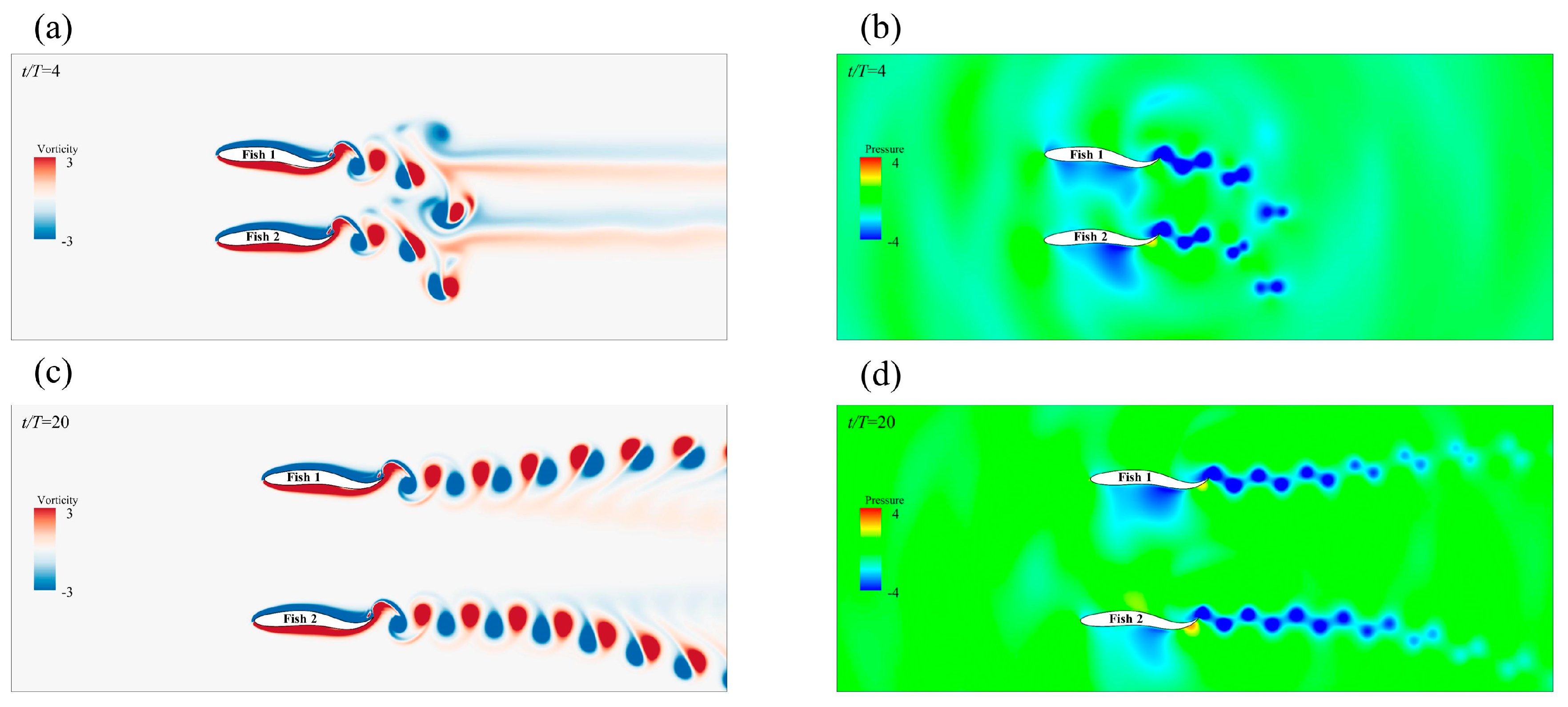
3.2.1. The Side−by−Side Formation
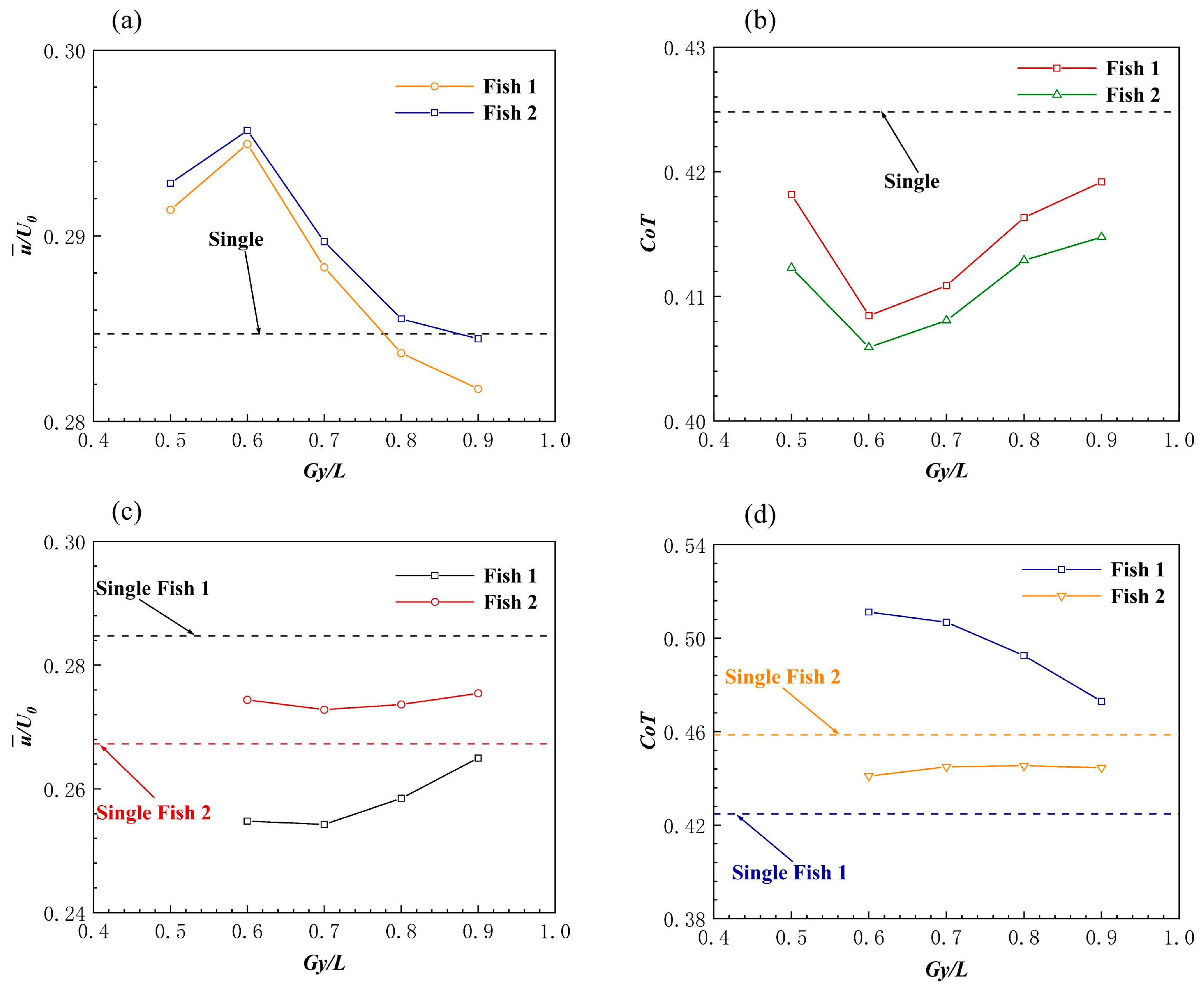
Effect of the Side-by-Side Formation on Swimming Speed
Effect of the Side-by-Side Formation on Energy Efficiency
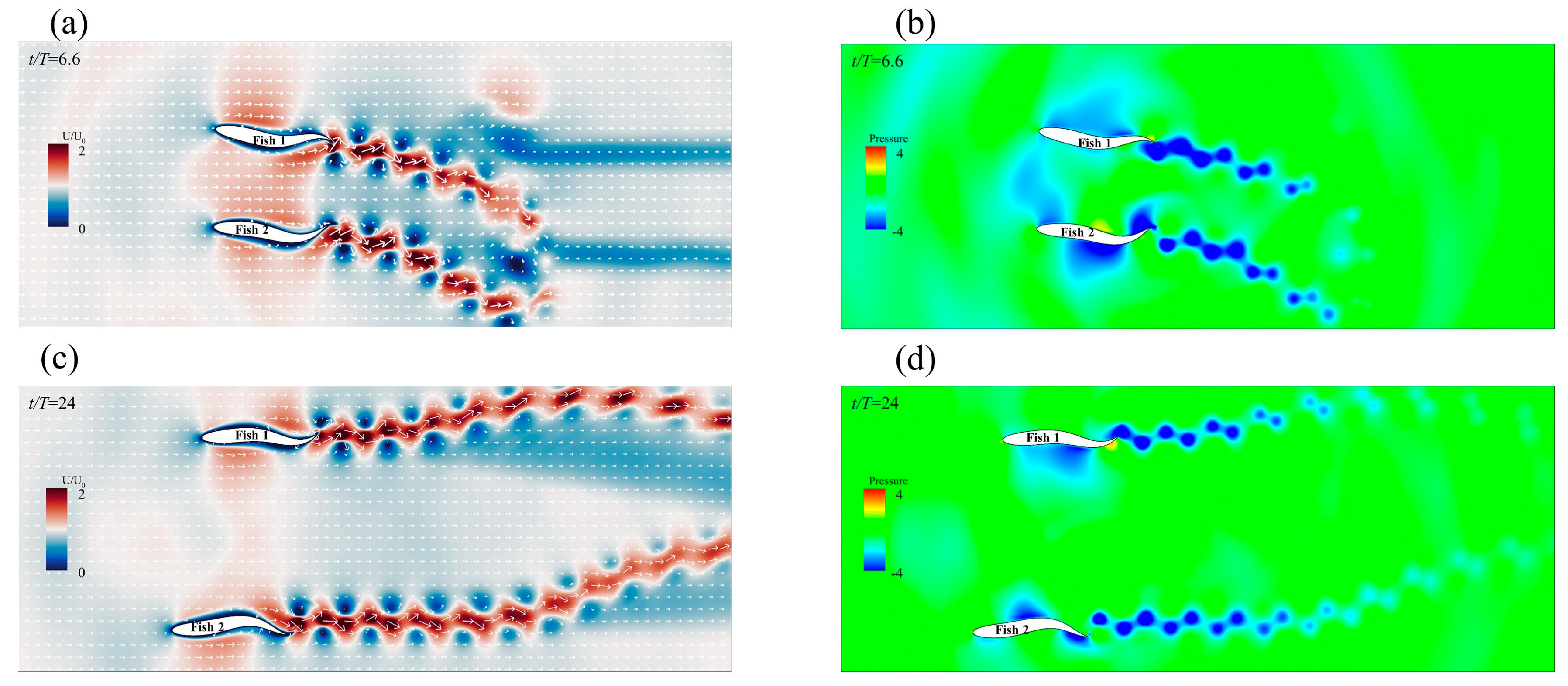
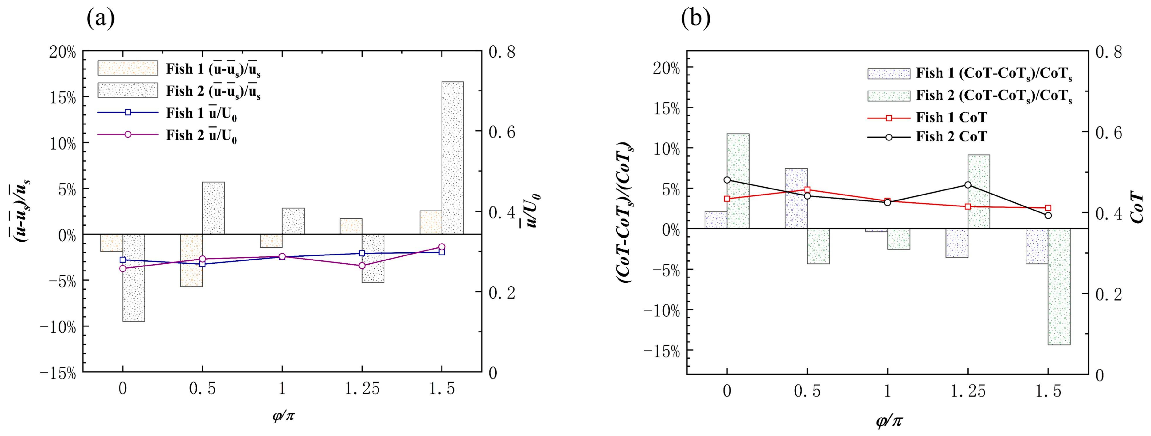
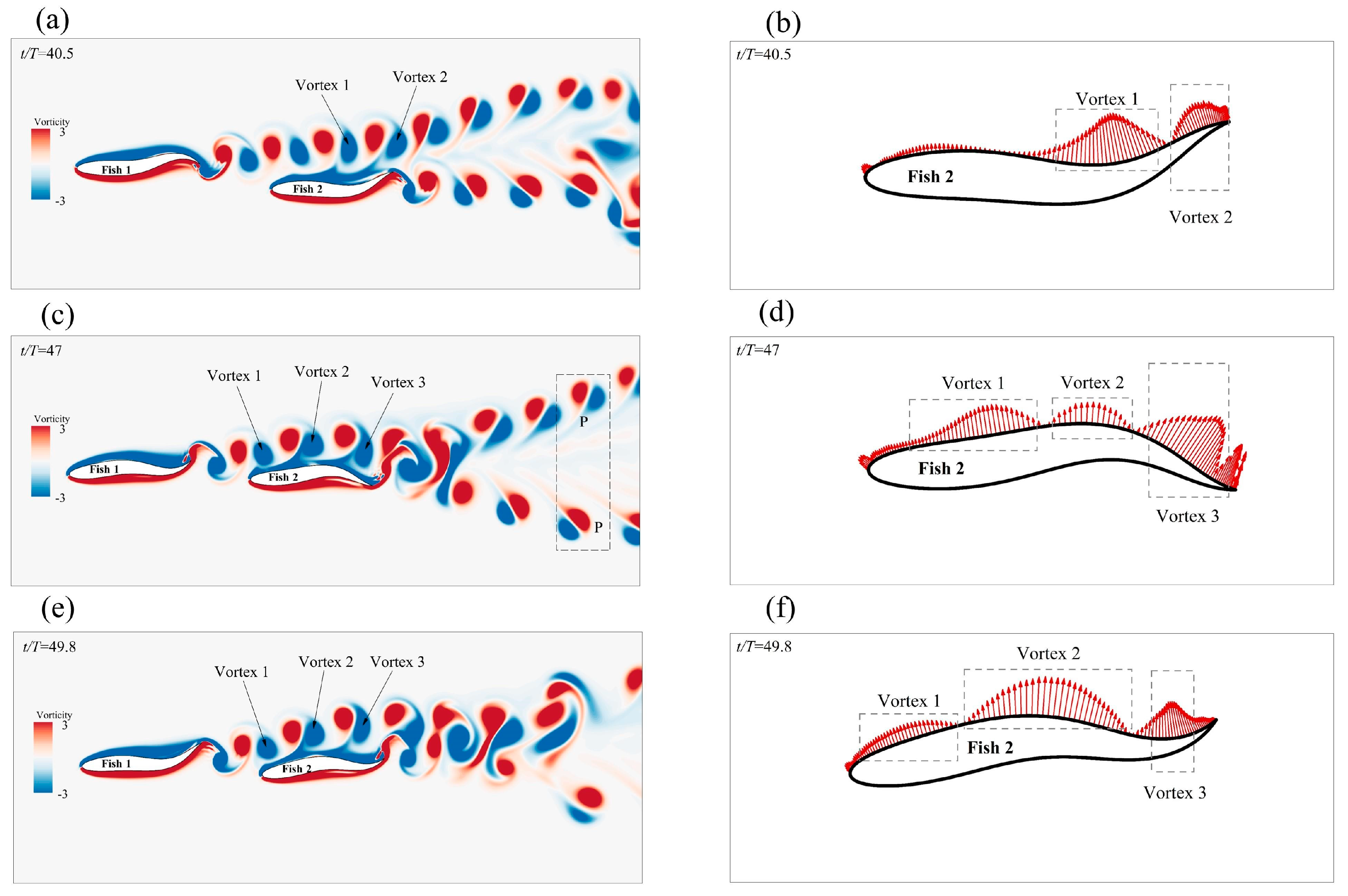
3.2.2. The Staggered Formation
Effects of the Staggered Formation on Swimming Speed
Effect of the Staggered Formation on Energy Efficiency
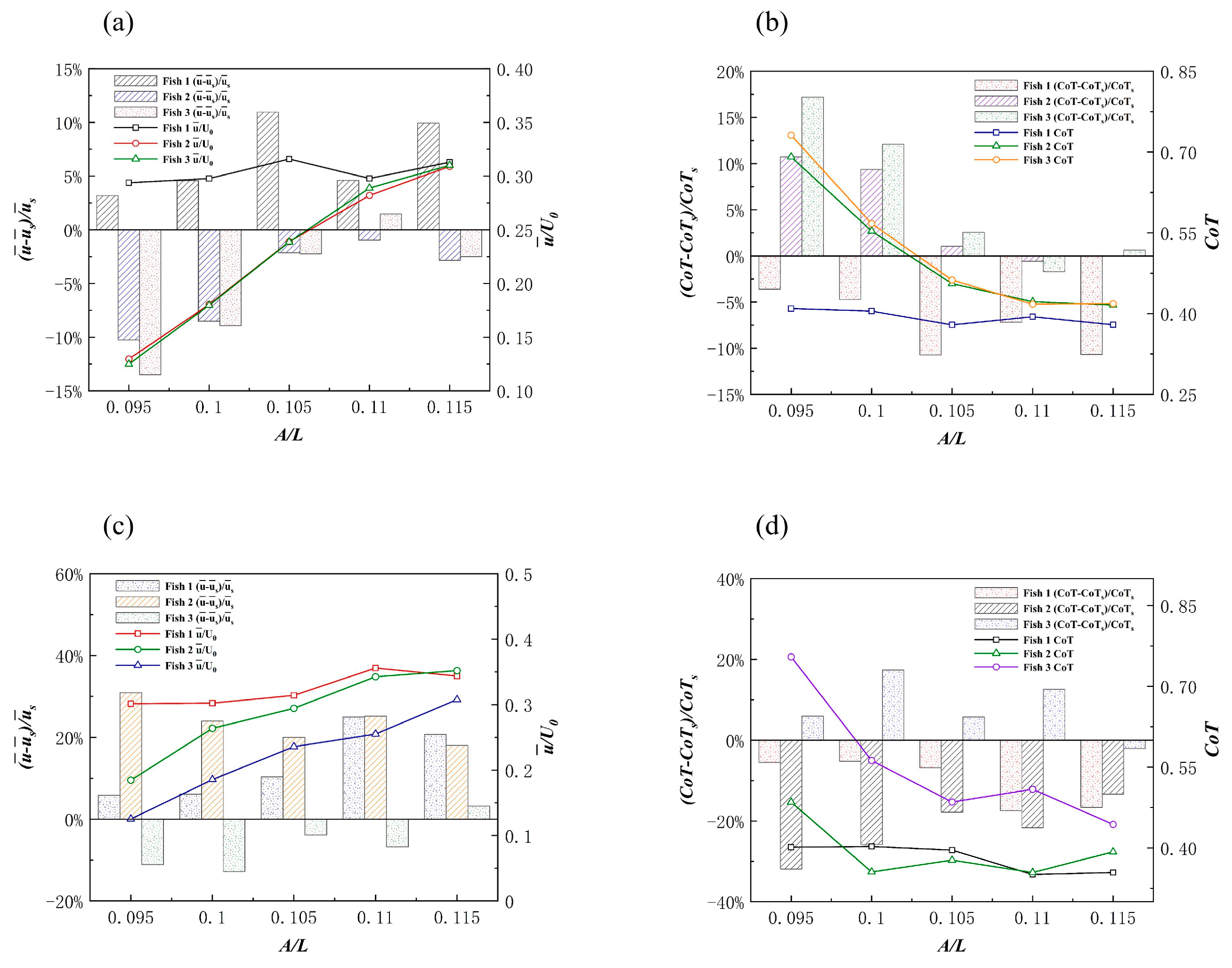
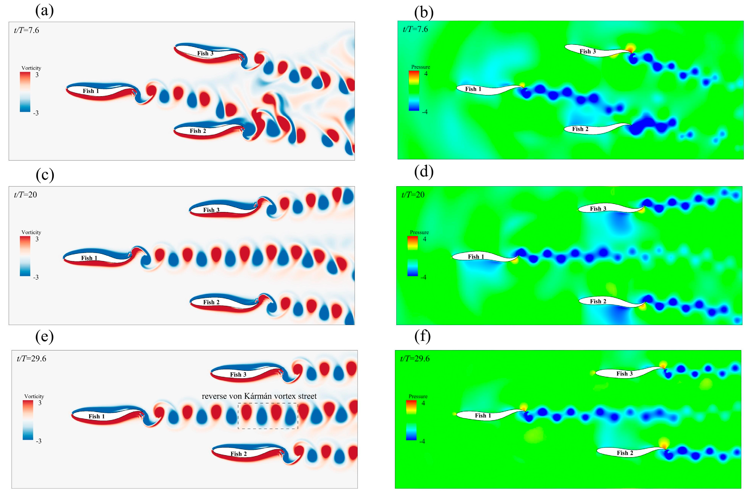
3.2.3. The Triangle Formation
Effects of the Triangle Formation on Swimming Speed
Effects of the Triangle Formation on Energy Efficiency
3.3. Discussion on the Simulation Results
4. Conclusions
Author Contributions
Funding
Data Availability Statement
Conflicts of Interest
References
- Larsson, M. Why do fish school? Curr. Zool. 2012, 58, 116–128. [Google Scholar] [CrossRef]
- Pitcher, T.J.; Magurran, A.E.; Winfield, I.J. Fish in larger shoals find food faster. Behav. Ecol. Sociobiol. 1982, 10, 149–151. [Google Scholar] [CrossRef]
- Parker, F.R., Jr. Reduced Metabolic Rates in Fishes as a Result of Induced Schooling. Trans. Am. Fish. Soc. 1973, 102, 125–131. [Google Scholar] [CrossRef]
- Fish, F. Energetics of swimming and flying in formation. Comments Theor. Biol. 1999, 5, 283–304. [Google Scholar]
- Killen, S.S.; Marras, S.; Steffensen, J.F.; McKenzie, D.J. Aerobic capacity influences the spatial position of individuals within fish schools. Proc. Biol. Sci. 2012, 279, 357–364. [Google Scholar] [CrossRef] [PubMed]
- Marras, S.; Killen, S.S.; Lindström, J.; McKenzie, D.J.; Steffensen, J.F.; Domenici, P. Fish swimming in schools save energy regardless of their spatial position. Behav. Ecol. Sociobiol. 2015, 69, 219–226. [Google Scholar] [CrossRef]
- Becker, A.D.; Masoud, H.; Newbolt, J.W.; Shelley, M.; Ristroph, L. Hydrodynamic schooling of flapping swimmers. Nat. Commun. 2015, 6, 8514. [Google Scholar] [CrossRef] [PubMed]
- Weihs, D. Hydromechanics of Fish Schooling. Nature 1973, 241, 290–291. [Google Scholar] [CrossRef]
- Verma, S.; Novati, G.; Koumoutsakos, P. Efficient collective swimming by harnessing vortices through deep reinforcement learning. Proc. Natl. Acad. Sci. USA 2018, 115, 5849–5854. [Google Scholar] [CrossRef]
- Liao, J.C.; Beal, D.N.; Lauder, G.V.; Triantafyllou, M.S. Fish exploiting vortices decrease muscle activity. Science 2003, 302, 1566–1569. [Google Scholar] [CrossRef]
- Svendsen, J.C.; Skov, J.; Bildsoe, M.; Steffensen, J.F. Intra-school positional preference and reduced tail beat frequency in trailing positions in schooling roach under experimental conditions. J. Fish Biol. 2003, 62, 834–846. [Google Scholar] [CrossRef]
- Dong, G.-J.; Lu, X.-Y. Characteristics of flow over traveling wavy foils in a side-by-side arrangement. Phys. Fluids 2007, 19, 057107. [Google Scholar] [CrossRef]
- Zheng, H.; Xie, F.; Zheng, Y.; Ji, T.; Zhu, Z. Propulsion performance of a two-dimensional flapping airfoil with wake map and dynamic mode decomposition analysis. Phys. Rev. E 2019, 99, 063109. [Google Scholar] [CrossRef]
- Zhu, Y.; Tian, F.-B.; Young, J.; Liao, J.C.; Lai, J.C.S. A numerical study of fish adaption behaviors in complex environments with a deep reinforcement learning and immersed boundary–lattice Boltzmann method. Sci. Rep. 2021, 11, 1691. [Google Scholar] [CrossRef]
- Arranz, G.; Flores, O.; García-Villalba, M. Flow interaction of three-dimensional self-propelled flexible plates in tandem. J. Fluid Mech. 2022, 931, A5. [Google Scholar] [CrossRef]
- Yu, H.; Liu, B.; Wang, C.; Liu, X.; Lu, X.Y.; Huang, H. Deep-reinforcement-learning-based self-organization of freely undulatory swimmers. Phys. Rev. E 2022, 105, 045105. [Google Scholar] [CrossRef] [PubMed]
- Li, S.; Chao, L.; Xu, L.; Yang, W.; Chen, X. Numerical Simulation and Analysis of Fish-Like Robots Swarm. Appl. Sci. 2019, 9, 1652. [Google Scholar] [CrossRef]
- Pan, Y.; Dong, H. Effects of phase difference on hydrodynamic interactions and wake patterns in high-density fish schools. Phys. Fluids 2022, 34, 111902. [Google Scholar] [CrossRef]
- Oza, A.U.; Ristroph, L.; Shelley, M.J. Lattices of Hydrodynamically Interacting Flapping Swimmers. Phys. Rev. X 2019, 9, 041024. [Google Scholar] [CrossRef]
- Heathcote, S.; Gursul, I. Flexible Flapping Airfoil Propulsion at Low Reynolds Numbers. AIAA J. 2007, 45, 1066–1079. [Google Scholar] [CrossRef]
- Lin, T.; Xia, W.; Hu, S. Effect of chordwise deformation on propulsive performance of flapping wings in forward flight. Aeronaut. J. 2021, 125, 430–451. [Google Scholar] [CrossRef]
- Lin, T.; Xia, W.; Pecora, R.; Wang, K.; Hu, S. Performance improvement of flapping propulsions from spanwise bending on a low-aspect-ratio foil. Ocean Eng. 2023, 284, 115305. [Google Scholar] [CrossRef]
- Afra, B.; Karimnejad, S.; Amiri Delouei, A.; Tarokh, A. Flow control of two tandem cylinders by a highly flexible filament: Lattice spring IB-LBM. Ocean Eng. 2022, 250, 111025. [Google Scholar] [CrossRef]
- Afra, B.; Delouei, A.A.; Tarokh, A. Flow-Induced Locomotion of a Flexible Filament in the Wake of a Cylinder in Non-Newtonian Flows. Int. J. Mech. Sci. 2022, 234, 107693. [Google Scholar] [CrossRef]
- Wei, C.; Hu, Q.; Li, S.; Shi, X. Hydrodynamic interactions and wake dynamics of fish schooling in rectangle and diamond formations. Ocean Eng. 2023, 267, 113258. [Google Scholar] [CrossRef]
- Kurt, M.; Ormonde, P.C.; Mivehchi, A.; Moored, K.W. Two-dimensionally stable self-organization arises in simple schooling swimmers through hydrodynamic interactions. arXiv 2021, arXiv:2102.03571. [Google Scholar]
- Kang, Q.; Lichtner, P.; Janecky, D. Lattice Boltzmann Method for Reacting Flows in Porous Media. Adv. Appl. Math. Mech. 2010, 2, 545–563. [Google Scholar] [CrossRef]
- Aidun, C.K.; Clausen, J.R. Lattice-Boltzmann method for complex flows. Annu. Rev. Fluid Mech. 2010, 42, 439–472. [Google Scholar] [CrossRef]
- Tao, S.; Zhang, H.; Guo, Z.; Wang, L.-P. Numerical investigation of dilute aerosol particle transport and deposition in oscillating multi-cylinder obstructions. Adv. Powder Technol. 2018, 29, 2003–2018. [Google Scholar] [CrossRef]
- Lallemand, P.; Luo, L.S. Theory of the lattice boltzmann method: Dispersion, dissipation, isotropy, galilean invariance, and stability. Phys. Rev. E Stat. Phys. Plasmas Fluids Relat. Interdiscip. Top. 2000, 61 Pt A, 6546–6562. [Google Scholar] [CrossRef]
- Tao, S.; He, Q.; Chen, J.; Chen, B.; Yang, G.; Wu, Z. A non-iterative immersed boundary-lattice Boltzmann method with boundary condition enforced for fluid–solid flows. Appl. Math. Model. 2019, 76, 362–379. [Google Scholar] [CrossRef]
- Tao, S.; Wang, L.; He, Q.; Chen, J.; Luo, J. Lattice Boltzmann simulation of complex thermal flows via a simplified immersed boundary method. J. Comput. Sci. 2022, 65, 101878. [Google Scholar] [CrossRef]
- Karimnejad, S.; Amiri Delouei, A.; Nazari, M.; Shahmardan, M.M.; Mohamad, A.A. Sedimentation of elliptical particles using Immersed Boundary—Lattice Boltzmann Method: A complementary repulsive force model. J. Mol. Liq. 2018, 262, 180–193. [Google Scholar] [CrossRef]
- Xu, L.; Wang, L.; Tian, F.-B.; Young, J.; Lai, J.C. A geometry-adaptive immersed boundary–lattice Boltzmann method for modelling fluid–structure interaction problems. In IUTAM Symposium on Recent Advances in Moving Boundary Problems in Mechanics; Springer: Berlin/Heidelberg, Germany, 2019; pp. 143–153. [Google Scholar]
- Lin, X.; Wu, J.; Zhang, T.; Yang, L. Phase difference effect on collective locomotion of two tandem autopropelled flapping foils. Phys. Rev. Fluids 2019, 4, 054101. [Google Scholar] [CrossRef]
- Ashraf, I.; Godoy-Diana, R.; Halloy, J.; Collignon, B.; Thiria, B. Synchronization and collective swimming patterns in fish (Hemigrammus bleheri). J. R. Soc. Interface 2016, 13, 20160734. [Google Scholar] [CrossRef]
- Pan, Y.; Dong, H. Computational analysis of hydrodynamic interactions in a high-density fish school. Phys. Fluids 2020, 32, 121901. [Google Scholar] [CrossRef]
- Yang, D.; Wu, J. Hydrodynamic Interaction of Two Self-Propelled Fish Swimming in a Tandem Arrangement. Fluids 2022, 7, 208. [Google Scholar] [CrossRef]
- Li, G.; Kolomenskiy, D.; Liu, H.; Thiria, B.; Godoy-Diana, R. On the energetics and stability of a minimal fish school. PLoS ONE 2019, 14, e0215265. [Google Scholar] [CrossRef]
- Videler, J.J. Fish Swimming; Chapman & Hall: London, UK, 1993; Volume 10. [Google Scholar]
- Tian, F.-B.; Lu, X.-Y.; Luo, H. Propulsive performance of a body with a traveling-wave surface. Phys. Rev. E 2012, 86, 016304. [Google Scholar] [CrossRef]
- Zhu, Y.; Pang, J.-H.; Gao, T.; Tian, F.-B. Learning to school in dense configurations with multi-agent deep reinforcement learning. Bioinspir. Biomim. 2023, 18, 015003. [Google Scholar] [CrossRef]
- Williamson, C.H.K. Defining a universal and continuous Strouhal–Reynolds number relationship for the laminar vortex shedding of a circular cylinder. Phys. Fluids 1988, 31, 2742–2744. [Google Scholar] [CrossRef]
- Norberg, C. Fluctuating lift on a circular cylinder: Review and new measurements. J. Fluids Struct. 2003, 17, 57–96. [Google Scholar] [CrossRef]
- Jiang, H.; Cheng, L. Strouhal–Reynolds number relationship for flow past a circular cylinder. J. Fluid Mech. 2017, 832, 170–188. [Google Scholar] [CrossRef]
- Linnick, M.N.; Fasel, H.F. A high-order immersed interface method for simulating unsteady incompressible flows on irregular domains. J. Comput. Phys. 2005, 204, 157–192. [Google Scholar] [CrossRef]
- Liu, C.; Zheng, X.; Sung, C.H. Preconditioned Multigrid Methods for Unsteady Incompressible Flows. J. Comput. Phys. 1998, 139, 35–57. [Google Scholar] [CrossRef]
- De Rosis, A.; Lévêque, E. Central-moment lattice Boltzmann schemes with fixed and moving immersed boundaries. Comput. Math. Appl. 2016, 72, 1616–1628. [Google Scholar] [CrossRef]
- Russell, D.; Wang, Z.J. A cartesian grid method for modeling multiple moving objects in 2D incompressible viscous flow. J. Comput. Phys. 2003, 191, 177–205. [Google Scholar] [CrossRef]
- Suzuki, K.; Inamuro, T. Effect of internal mass in the simulation of a moving body by the immersed boundary method. Comput. Fluids 2011, 49, 173–187. [Google Scholar] [CrossRef]
- DÜTsch, H.; Durst, F.; Becker, S.; Lienhart, H. Low-Reynolds-number flow around an oscillating circular cylinder at low Keulegan–Carpenter numbers. J. Fluid Mech. 1998, 360, 249–271. [Google Scholar] [CrossRef]
- Liao, C.-C.; Chang, Y.-W.; Lin, C.-A.; McDonough, J.M. Simulating flows with moving rigid boundary using immersed-boundary method. Comput. Fluids 2010, 39, 152–167. [Google Scholar] [CrossRef]
- Kern, S.; Koumoutsakos, P. Simulations of optimized anguilliform swimming. J. Exp. Biol. 2006, 209 Pt 24, 4841–4857. [Google Scholar] [CrossRef] [PubMed]
- Gazzola, M.; Chatelain, P.; van Rees, W.M.; Koumoutsakos, P. Simulations of single and multiple swimmers with non-divergence free deforming geometries. J. Comput. Phys. 2011, 230, 7093–7114. [Google Scholar] [CrossRef]
- Wei, C.; Hu, Q.; Zhang, T.; Zeng, Y. Passive hydrodynamic interactions in minimal fish schools. Ocean Eng. 2022, 247, 110574. [Google Scholar] [CrossRef]
- Novati, G.; Verma, S.; Alexeev, D.; Rossinelli, D.; van Rees, W.M.; Koumoutsakos, P. Synchronisation through learning for two self-propelled swimmers. Bioinspiration Biomim. 2017, 12, 036001. [Google Scholar] [CrossRef] [PubMed]
- Hemelrijk, C.; Reid, D.; Hildenbrandt, H.; Padding, J. The increased efficiency of fish swimming in a school. Fish Fish. 2013, 16, 511–521. [Google Scholar] [CrossRef]
- Ren, K.; Yu, J.; Chen, Z.; Li, H.; Feng, H.; Liu, K. Numerical investigation on energetically advantageous formations and swimming modes using two self-propelled fish. Ocean Eng. 2023, 267, 113288. [Google Scholar] [CrossRef]
- Son, Y.; Lee, J.H. Flapping dynamics of coupled flexible flags in a uniform viscous flow. J. Fluids Struct. 2017, 68, 339–355. [Google Scholar] [CrossRef]


| Formation Type | Geometric Figure | Gx (L) | Gy (L) | φ (π) | A (L) |
|---|---|---|---|---|---|
| Side-by-side |  | 0 | 0.5, 0.6, 0.7, 0.8, 0.9 | 0, 1.5 | 0.11 |
| Interlace |  | 1.6 | 0.6 | 0, 0.5, 1.0, 1.25, 1.5 | 0.11 |
| Triangle | 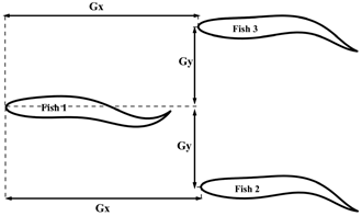 | 1.4 | 0.4 | 0, 1.5 | 0.095, 0.10, 0.105, 0.11, 0.115 |
Disclaimer/Publisher’s Note: The statements, opinions and data contained in all publications are solely those of the individual author(s) and contributor(s) and not of MDPI and/or the editor(s). MDPI and/or the editor(s) disclaim responsibility for any injury to people or property resulting from any ideas, methods, instructions or products referred to in the content. |
© 2023 by the authors. Licensee MDPI, Basel, Switzerland. This article is an open access article distributed under the terms and conditions of the Creative Commons Attribution (CC BY) license (https://creativecommons.org/licenses/by/4.0/).
Share and Cite
Zhang, F.; Pang, J.; Wu, Z.; Liu, J.; Zhong, Y. Effects of Different Motion Parameters on the Interaction of Fish School Subsystems. Biomimetics 2023, 8, 510. https://doi.org/10.3390/biomimetics8070510
Zhang F, Pang J, Wu Z, Liu J, Zhong Y. Effects of Different Motion Parameters on the Interaction of Fish School Subsystems. Biomimetics. 2023; 8(7):510. https://doi.org/10.3390/biomimetics8070510
Chicago/Turabian StyleZhang, Feihu, Jianhua Pang, Zongduo Wu, Junkai Liu, and Yifei Zhong. 2023. "Effects of Different Motion Parameters on the Interaction of Fish School Subsystems" Biomimetics 8, no. 7: 510. https://doi.org/10.3390/biomimetics8070510
APA StyleZhang, F., Pang, J., Wu, Z., Liu, J., & Zhong, Y. (2023). Effects of Different Motion Parameters on the Interaction of Fish School Subsystems. Biomimetics, 8(7), 510. https://doi.org/10.3390/biomimetics8070510