
A Reinforcement Learning-Based Bi-Population Nutcracker Optimizer for Global Optimization


Abstract

1. Introduction
- An RL-based bi-population nutcracker optimizer algorithm (RLNOA) is developed to solve complex optimization problems;
- The foraging strategy of the NOA is enhanced using ROBL, improving its ability to search for feasible solutions;
- Q-learning is utilized to control the selection of the most appropriate exploitation strategy for each iteration, dynamically improving the refinement of the optimal solution.
2. Preliminaries
2.1. Nutcracker Optimization Algorithm
2.1.1. Foraging and Storage Strategies
2.1.2. Cache Search and Recovery Strategies
2.2. Reinforcement Learning
3. The Development of the Proposed Algorithm
3.1. Overview
| Algorithm 1: The pseudocode of the RLNOA |
| Learning rate Discount factor , , . Set the initial Q-table: Q(s, a) = 0 Set t = 1 While t < Tmax do Acquire sub-population by Equation (19) belong to exploration sub-population by Equation (16) Else Determine the state of the exploitation sub-population by Equations (20) and (21) Choose the best a for the current s from Q-table Switch action Case 1: Storage by Equation (4) Case 2: Recovery by Equation (13) End Switch Set the reward by Equation (25) End if if its fitness is improved End for Calculate the relative changes of fitness and local diversity for the population Update Q-table by the exploitation sub-population t = t + 1 End While Return results Terminate |
3.2. ROBL-Based Foraging Strategy
3.3. Q-Learning-Based Exploitation Behavior
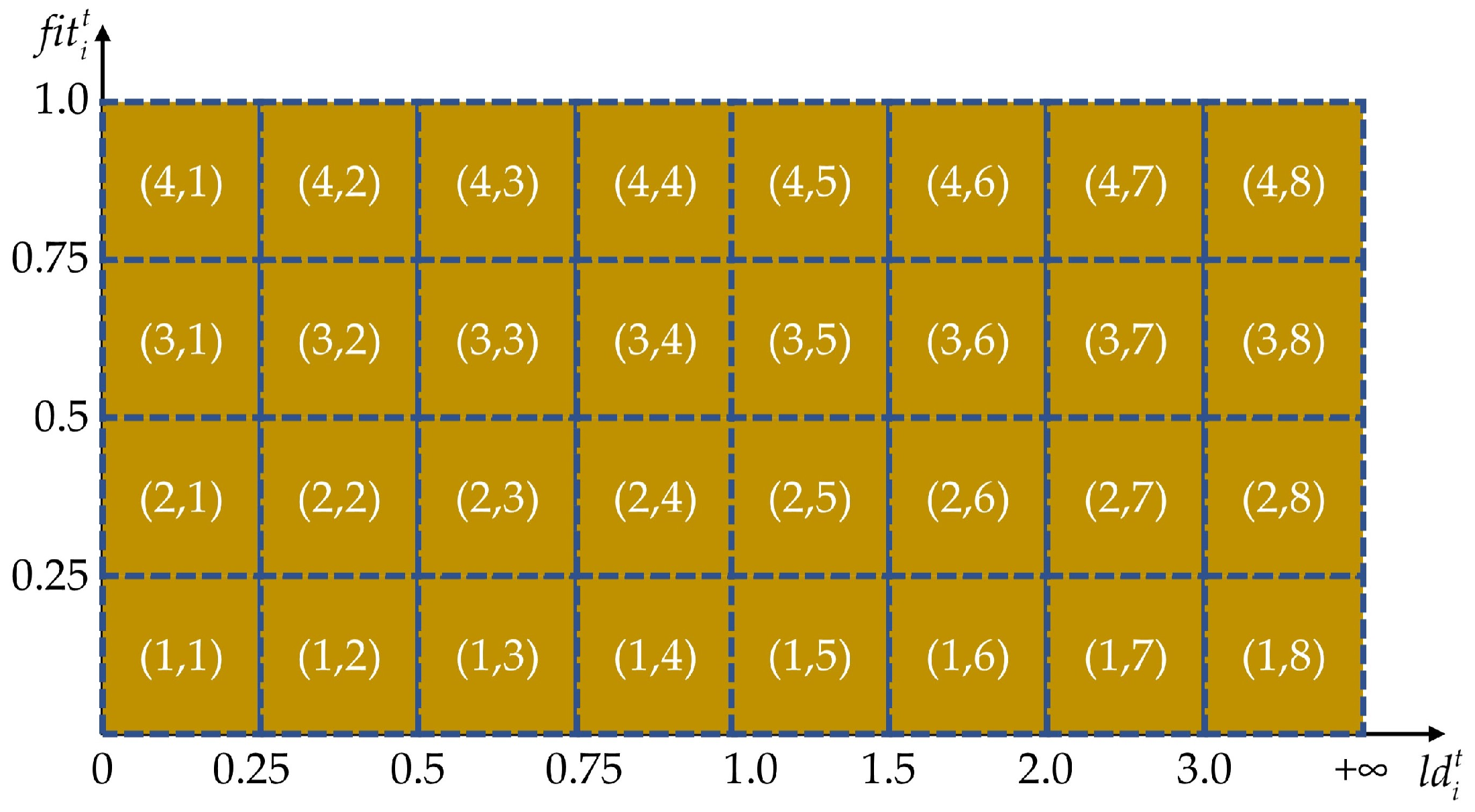
3.3.1. State Encoding
3.3.2. Action Options
3.3.3. Reward Options
3.4. Time Complexity
4. Experimental Results
4.1. Test Conditions
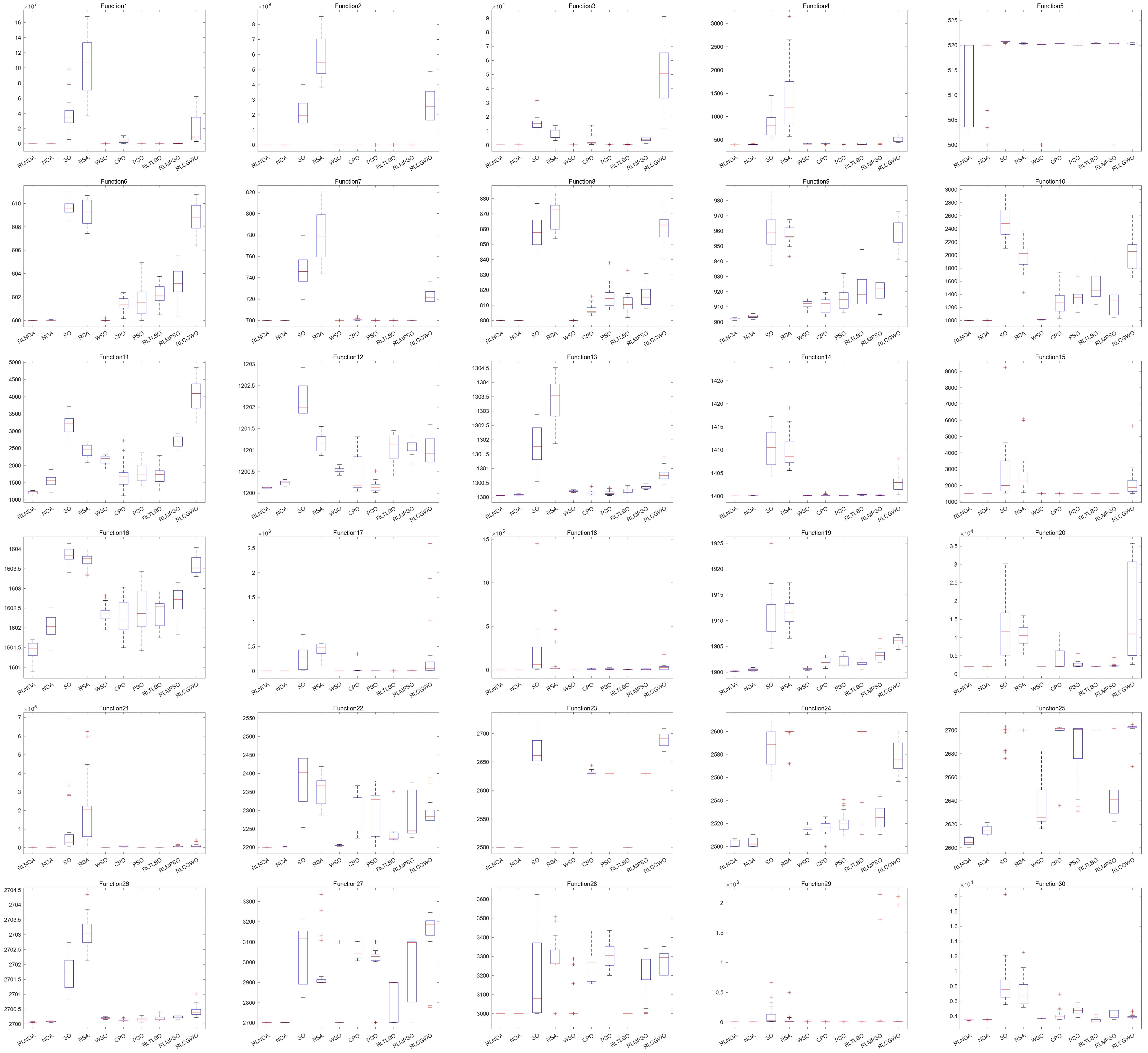
4.2. Comparison over CEC-2014
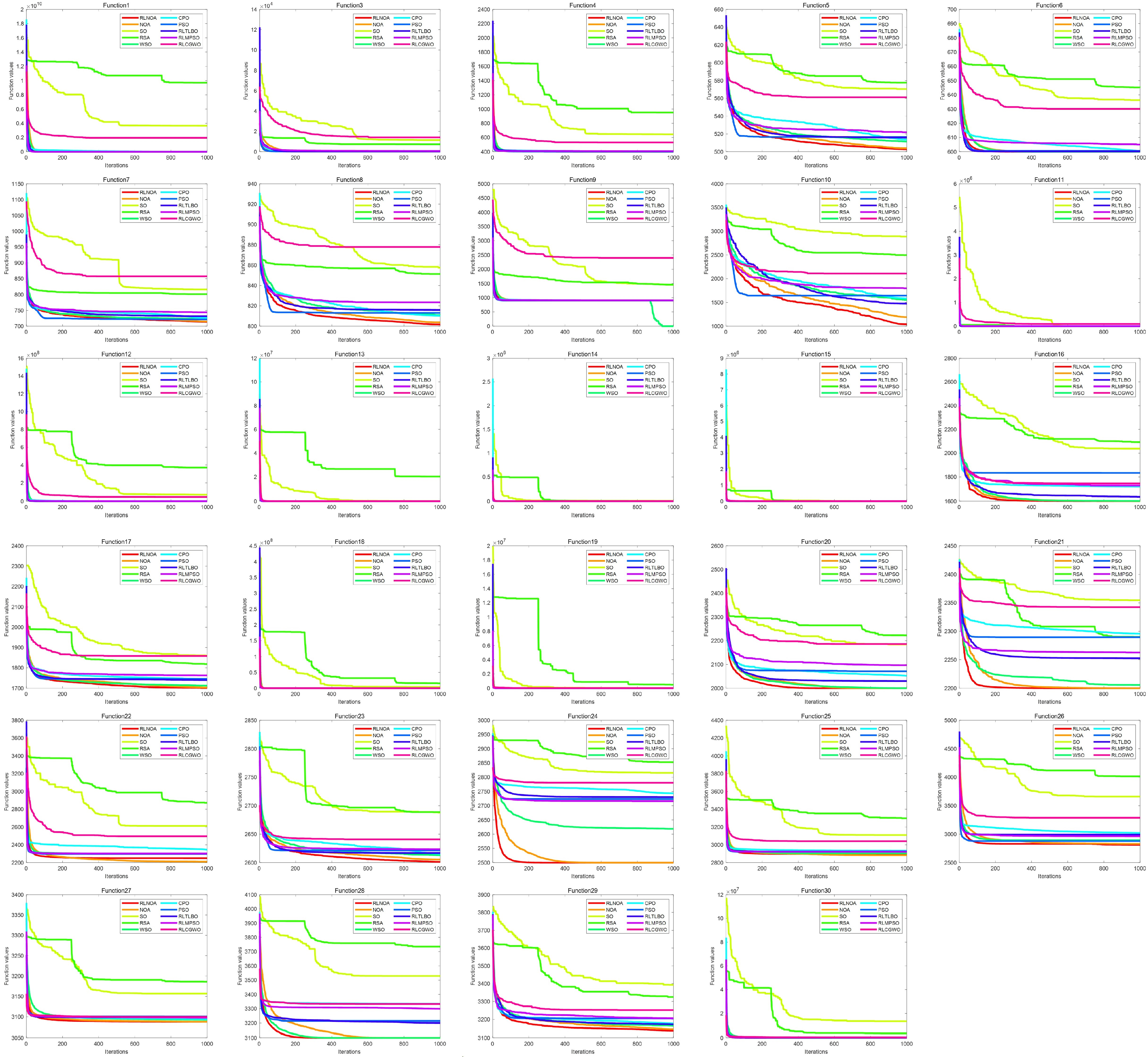
4.3. Comparison over CEC-2017
4.4. Comparison over CEC-2020
4.5. Analysis of the Q-Table
4.6. Analysis of the RLNOA’s Parameters
- Global exploration threshold : to verify the effect of on the efficiency of the RLNOA, experiments are performed for several values of , taken as 0.2, 0.4, 0.6, and 0.8, while other parameters are unchanged. As shown in Table 5, the RLNOA is insensitive to this parameter. The results of F17 indicate that the RLNOA performs best when is set to a specific value.
- Control parameter : experiments are performed for several values of , taken as 0.05, 0.1, 0.2, and 0.5, while other parameters are unchanged. As shown in Table 6, the RLNOA is not sensitive to small changes in the parameter .
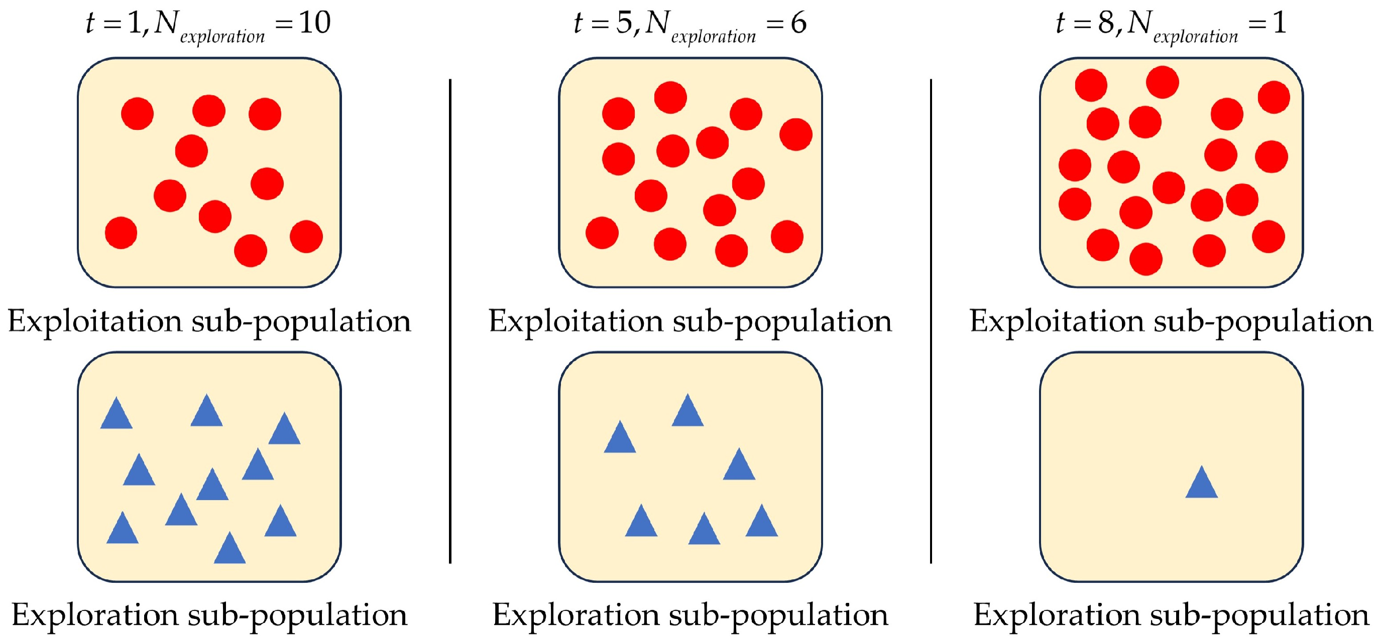
- Control parameter : to explore the sensitivity of the RLNOA to the parameter , experiments are caried out for different values of , as shown in Table 8. It is apparent that the RLNOA is sensitive to . This is primarily because controls the variation trend of the exploration sub-population during the optimization process. Table 8 also shows that the RLNOA acquires the best results when the value of is set to 1.
5. Conclusions
Author Contributions
Funding
Institutional Review Board Statement
Informed Consent Statement
Data Availability Statement
Conflicts of Interest
Appendix A

| Indices | A, B, and C | Integers randomly selected in the range of [0, NP] | |
| Index of individuals in the population | The lower bound of the optimization problem in the jth dimension | ||
| Index of dimensions | NP | The population size | |
| Index of individuals in the neighborhood set | A probability value | ||
| Index of iteration | A global exploration threshold | ||
| Sets | The maximum iterations | ||
| The population in the iteration | The upper bound of the optimization problem in the jth dimension | ||
| The neighborhood set of | Variables | ||
| Parameters | and | The current and next actions respectively | |
| The learning rate | The relative changes of fitness value | ||
| The discount factor | The relative changes of local diversity | ||
| and | Control parameter | and | The current and next states respectively |
| , , and | A parameter generated by the levy flight | The new position of the ith individual generated in the foraging phase | |
| A parameter chosen in the range of [0, ] | The jth dimension of the ith individual in the iteration | ||
| and | A parameter that linearly decreased from 1 to 0 | The new position of the ith individual generated in the storage phase | |
| A random number selected within the range [0, 1] | The mean position of the jth dimensions for current population in the iteration | ||
| A random number generated based on a normal distribution | The local diversity of individual | ||
| The dimension of the search space | The size of the exploration sub-population | ||
| The number of near neighbors | The corresponding value in the Q-table | ||
| and | Random numbers selected within the range [0, 1] | The reward acquired after performing action | |
| An integer chosen randomly between zero and one |
References
- Hubálovsky, S.; Hubálovská, M.; Matousová, I. A New Hybrid Particle Swarm Optimization-Teaching-Learning-Based Optimization for Solving Optimization Problems. Biomimetics 2024, 9, 8. [Google Scholar] [CrossRef] [PubMed]
- Wang, R.T.; Zhang, S.S.; Zou, G.Y. An Improved Multi-Strategy Crayfish Optimization Algorithm for Solving Numerical Optimization Problems. Biomimetics 2024, 9, 361. [Google Scholar] [CrossRef] [PubMed]
- Pardo, X.C.; González, P.; Banga, J.R.; Doallo, R. Population based metaheuristics in Spark: Towards a general framework using PSO as a case study. Swarm Evol. Comput. 2024, 85, 101483. [Google Scholar] [CrossRef]
- Tatsis, V.A.; Parsopoulos, K.E. Reinforcement learning for enhanced online gradient-based parameter adaptation in metaheuristics. Swarm Evol. Comput. 2023, 83, 101371. [Google Scholar] [CrossRef]
- Wang, Y.; Xiong, G.J.; Xu, S.P.; Suganthan, P.N. Large-scale power system multi-area economic dispatch considering valve point effects with comprehensive learning differential evolution. Swarm Evol. Comput. 2024, 89, 101620. [Google Scholar] [CrossRef]
- Zhang, Z.; Zhang, H.F.; Tian, Y.Z.; Li, C.W.; Yue, D. Cooperative constrained multi-objective dual-population evolutionary algorithm for optimal dispatching of wind-power integrated power system. Swarm Evol. Comput. 2024, 87, 101525. [Google Scholar] [CrossRef]
- Feng, X.; Pan, A.Q.; Ren, Z.Y.; Hong, J.C.; Fan, Z.P.; Tong, Y.H. An adaptive dual-population based evolutionary algorithm for industrial cut tobacco drying system. Appl. Soft Comput. 2023, 144, 110446. [Google Scholar] [CrossRef]
- Luo, T.; Xie, J.P.; Zhang, B.T.; Zhang, Y.; Li, C.Q.; Zhou, J. An improved levy chaotic particle swarm optimization algorithm for energy-efficient cluster routing scheme in industrial wireless sensor networks. Expert Syst. Appl. 2024, 241, 122780. [Google Scholar] [CrossRef]
- Qu, C.Z.; Gai, W.D.; Zhang, J.; Zhong, M.Y. A novel hybrid grey wolf optimizer algorithm for unmanned aerial vehicle (UAV) path planning. Knowl.-Based Syst. 2020, 194, 105530. [Google Scholar] [CrossRef]
- Qu, C.Z.; Gai, W.D.; Zhong, M.Y.; Zhang, J. A novel reinforcement learning based grey wolf optimizer algorithm for unmanned aerial vehicles (UAVs) path planning. Appl. Soft Comput. 2020, 89, 106099. [Google Scholar] [CrossRef]
- Qu, C.; Zhang, Y.; Ma, F.; Huang, K. Parameter optimization for point clouds denoising based on no-reference quality assessment. Measurement 2023, 211, 112592. [Google Scholar] [CrossRef]
- Chauhan, D.; Yadav, A. An archive-based self-adaptive artificial electric field algorithm with orthogonal initialization for real-parameter optimization problems. Appl. Soft Comput. 2024, 150, 111109. [Google Scholar] [CrossRef]
- Li, G.Q.; Zhang, W.W.; Yue, C.T.; Wang, Y.R. Balancing exploration and exploitation in dynamic constrained multimodal multi-objective co-evolutionary algorithm. Swarm Evol. Comput. 2024, 89, 101652. [Google Scholar] [CrossRef]
- Ahadzadeh, B.; Abdar, M.; Safara, F.; Khosravi, A.; Menhaj, M.B.; Suganthan, P.N. SFE: A Simple, Fast, and Efficient Feature Selection Algorithm for High-Dimensional Data. IEEE Trans. Evol. Comput. 2023, 27, 1896–1911. [Google Scholar] [CrossRef]
- Fu, S.; Huang, H.; Ma, C.; Wei, J.; Li, Y.; Fu, Y. Improved dwarf mongoose optimization algorithm using novel nonlinear control and exploration strategies. Expert Syst. Appl. 2023, 233, 120904. [Google Scholar] [CrossRef]
- Li, J.; Li, G.; Wang, Z.; Cui, L. Differential evolution with an adaptive penalty coefficient mechanism and a search history exploitation mechanism. Expert Syst. Appl. 2023, 230, 120530. [Google Scholar] [CrossRef]
- Hu, C.; Zeng, S.; Li, C. A framework of global exploration and local exploitation using surrogates for expensive optimization. Knowl.-Based Syst. 2023, 280, 111018. [Google Scholar] [CrossRef]
- Chang, D.; Rao, C.; Xiao, X.; Hu, F.; Goh, M. Multiple strategies based Grey Wolf Optimizer for feature selection in performance evaluation of open-ended funds. Swarm Evol. Comput. 2024, 86, 101518. [Google Scholar] [CrossRef]
- Hashim, F.A.; Hussien, A.G. Snake Optimizer: A novel meta-heuristic optimization algorithm. Knowl.-Based Syst. 2022, 242, 108320. [Google Scholar] [CrossRef]
- Braik, M.; Hammouri, A.; Atwan, J.; Al-Betar, M.A.A.; Awadallah, M.A. White Shark Optimizer: A novel bio-inspired meta-heuristic algorithm for global optimization problems. Knowl.-Based Syst. 2022, 243, 108457. [Google Scholar] [CrossRef]
- Kumar, S.; Sharma, N.K.; Kumar, N. WSOmark: An adaptive dual-purpose color image watermarking using white shark optimizer and Levenberg-Marquardt BPNN. Expert Syst. Appl. 2023, 226, 120137. [Google Scholar] [CrossRef]
- Abualigah, L.; Abd Elaziz, M.; Sumari, P.; Geem, Z.W.; Gandomi, A.H. Reptile Search Algorithm (RSA): A nature-inspired meta-heuristic optimizer. Expert Syst. Appl. 2022, 191, 116158. [Google Scholar] [CrossRef]
- Abdel-Basset, M.; Mohamed, R.; Abouhawwash, M. Crested Porcupine Optimizer: A new nature-inspired metaheuristic. Knowl.-Based Syst. 2024, 284, 111257. [Google Scholar] [CrossRef]
- Abdel-Basset, M.; Mohamed, R.; Jameel, M.; Abouhawwash, M. Nutcracker optimizer: A novel nature-inspired metaheuristic algorithm for global optimization and engineering design problems. Knowl.-Based Syst. 2023, 262, 110248. [Google Scholar] [CrossRef]
- Qaraad, M.; Amjad, S.; Hussein, N.K.; Farag, M.A.; Mirjalili, S.; Elhosseini, M.A. Quadratic interpolation and a new local search approach to improve particle swarm optimization: Solar photovoltaic parameter estimation. Expert Syst. Appl. 2024, 236, 121417. [Google Scholar] [CrossRef]
- Ahmed, R.; Rangaiah, G.P.; Mahadzir, S.; Mirjalili, S.; Hassan, M.H.; Kamel, S. Memory, evolutionary operator, and local search based improved Grey Wolf Optimizer with linear population size reduction technique. Knowl.-Based Syst. 2023, 264, 110297. [Google Scholar] [CrossRef]
- Khosravi, H.; Amiri, B.; Yazdanjue, N.; Babaiyan, V. An improved group teaching optimization algorithm based on local search and chaotic map for feature selection in high-dimensional data. Expert Syst. Appl. 2022, 204, 117493. [Google Scholar] [CrossRef]
- Ekinci, S.; Izci, D.; Abualigah, L.; Abu Zitar, R. A Modified Oppositional Chaotic Local Search Strategy Based Aquila Optimizer to Design an Effective Controller for Vehicle Cruise Control System. J. Bionic Eng. 2023, 20, 1828–1851. [Google Scholar] [CrossRef]
- Xiao, J.; Wang, Y.J.; Xu, X.K. Fuzzy Community Detection Based on Elite Symbiotic Organisms Search and Node Neighborhood Information. IEEE Trans. Fuzzy Syst. 2022, 30, 2500–2514. [Google Scholar] [CrossRef]
- Zhu, Q.L.; Lin, Q.Z.; Li, J.Q.; Coello, C.A.C.; Ming, Z.; Chen, J.Y.; Zhang, J. An Elite Gene Guided Reproduction Operator for Many-Objective Optimization. IEEE Trans. Cybern. 2021, 51, 765–778. [Google Scholar] [CrossRef]
- Zhang, Y.Y. Elite archives-driven particle swarm optimization for large scale numerical optimization and its engineering applications. Swarm Evol. Comput. 2023, 76, 101212. [Google Scholar] [CrossRef]
- Zhong, X.X.; Cheng, P. An elite-guided hierarchical differential evolution algorithm. Appl. Intell. 2021, 51, 4962–4983. [Google Scholar] [CrossRef]
- Zhou, L.; Feng, L.; Gupta, A.; Ong, Y.S. Learnable Evolutionary Search Across Heterogeneous Problems via Kernelized Autoencoding. IEEE Trans. Evol. Comput. 2021, 25, 567–581. [Google Scholar] [CrossRef]
- Feng, L.; Zhou, W.; Liu, W.C.; Ong, Y.S.; Tan, K.C. Solving Dynamic Multiobjective Problem via Autoencoding Evolutionary Search. IEEE Trans. Cybern. 2022, 52, 2649–2662. [Google Scholar] [CrossRef]
- Zhan, Z.H.; Wang, Z.J.; Jin, H.; Zhang, J. Adaptive Distributed Differential Evolution. IEEE Trans. Cybern. 2020, 50, 4633–4647. [Google Scholar] [CrossRef]
- Zhan, Z.H.; Li, J.Y.; Kwong, S.; Zhang, J. Learning-Aided Evolution for Optimization. IEEE Trans. Evol. Comput. 2023, 27, 1794–1808. [Google Scholar] [CrossRef]
- Zabihi, Z.; Moghadam, A.M.E.; Rezvani, M.H. Reinforcement Learning Methods for Computation Offloading: A Systematic Review. Acm Comput. Surv. 2024, 56, 1–41. [Google Scholar] [CrossRef]
- Wang, D.; Gao, N.; Liu, D.; Li, J.; Lewis, F.L. Recent Progress in Reinforcement Learning and Adaptive Dynamic Programming for Advanced Control Applications. IEEE-CAA J. Autom. Sin. 2024, 11, 18–36. [Google Scholar] [CrossRef]
- Zhao, F.; Wang, Q.; Wang, L. An inverse reinforcement learning framework with the Q-learning mechanism for the metaheuristic algorithm. Knowl.-Based Syst. 2023, 265, 110368. [Google Scholar] [CrossRef]
- Ghetas, M.; Issa, M. A novel reinforcement learning-based reptile search algorithm for solving optimization problems. Neural Comput. Appl. 2023, 36, 533–568. [Google Scholar] [CrossRef]
- Li, Z.; Shi, L.; Yue, C.; Shang, Z.; Qu, B. Differential evolution based on reinforcement learning with fitness ranking for solving multimodal multiobjective problems. Swarm Evol. Comput. 2019, 49, 234–244. [Google Scholar] [CrossRef]
- Tan, Z.; Li, K. Differential evolution with mixed mutation strategy based on deep reinforcement learning. Appl. Soft Comput. 2021, 111, 107678. [Google Scholar] [CrossRef]
- Wu, D.; Wang, S.; Liu, Q.; Abualigah, L.; Jia, H. An Improved Teaching-Learning-Based Optimization Algorithm with Reinforcement Learning Strategy for Solving Optimization Problems. Comput. Intell. Neurosci. 2022, 2022, 1535957. [Google Scholar] [CrossRef] [PubMed]
- Samma, H.; Lim, C.P.; Saleh, J.M. A new Reinforcement Learning-Based Memetic Particle Swarm Optimizer. Appl. Soft Comput. 2016, 43, 276–297. [Google Scholar] [CrossRef]
- Hu, Z.P.; Yu, X.B. Reinforcement learning-based comprehensive learning grey wolf optimizer for feature selection. Appl. Soft Comput. 2023, 149, 110959. [Google Scholar] [CrossRef]
- Li, J.; Dong, H.; Wang, P.; Shen, J.; Qin, D. Multi-objective constrained black-box optimization algorithm based on feasible region localization and performance-improvement exploration. Appl. Soft Comput. 2023, 148, 110874. [Google Scholar] [CrossRef]
- Wang, Z.; Yao, S.; Li, G.; Zhang, Q. Multiobjective Combinatorial Optimization Using a Single Deep Reinforcement Learning Model. IEEE Trans. Cybern. 2024, 54, 1984–1996. [Google Scholar] [CrossRef]
- Huang, L.; Dong, B.; Xie, W.; Zhang, W. Offline Reinforcement Learning with Behavior Value Regularization. IEEE Trans. Cybern. 2024, 54, 3692–3704. [Google Scholar] [CrossRef]
- Abdel-Basset, M.; El-Shahat, D.; Jameel, M.; Abouhawwash, M. Exponential distribution optimizer (EDO): A novel math-inspired algorithm for global optimization and engineering problems. Artif. Intell. Rev. 2023, 56, 9329–9400. [Google Scholar] [CrossRef]


| Algorithm | Specifications | Population Size NP |
|---|---|---|
| RLNOA | 100 | |
| NOA | 100 | |
| SO | 100 | |
| RSA | 100 | |
| CPO | 100 | |
| GWO | Convergence constant decreases linearly from 2 to 0 | 100 |
| PSO | 100 | |
| RLTLBO | 33 because this algorithm has three main stages | |
| RLMPSO | is set as 0.2 of search range | 100 |
| RLCGWO | 100 |
| Fun | Metrics | RLNOA | NOA | SO | RSA | CPO | GWO | PSO | RLTLBO | RLMPSO | RLCGWO |
|---|---|---|---|---|---|---|---|---|---|---|---|
| F1 | Ave | 1.00 × 10² | 1.04 × 10² | 3.86 × 10⁷ | 1.02 × 10⁸ | 1.64 × 10² | 4.57 × 10⁶ | 1.24 × 10⁴ | 2.39 × 10⁴ | 3.28 × 10⁵ | 1.86 × 10⁷ |
| Std | 4.65 × 10⁻³ | 2.55 × 100 | 2.05 × 10⁷ | 4.09 × 10⁷ | 4.73 × 101 | 3.34 × 10⁶ | 1.33 × 10⁴ | 3.63 × 10⁴ | 2.44 × 10⁵ | 1.79 × 10⁷ | |
| Rank | 1 | 2 | 9 | 10 | 3 | 7 | 4 | 5 | 6 | 8 | |
| F2 | Ave | 2.00 × 10² | 2.00 × 10² | 2.16 × 10⁹ | 5.89 × 10⁹ | 2.00 × 10² | 6.15 × 10³ | 1.10 × 10³ | 5.83 × 10² | 2.04 × 10³ | 2.60 × 10⁹ |
| Std | 2.61 × 10⁻⁶ | 1.15 × 10⁻³ | 9.40 × 10⁸ | 1.50 × 10⁹ | 1.03 × 10⁻⁵ | 4.49 × 10³ | 1.17 × 10³ | 6.06 × 10² | 2.90 × 10³ | 1.26 × 10⁹ | |
| Rank | 1 | 3 | 8 | 10 | 2 | 7 | 5 | 4 | 6 | 9 | |
| F3 | Ave | 3.00 × 10² | 3.00 × 10² | 1.54 × 10⁴ | 8.05 × 10³ | 3.00 × 10² | 4.01 × 10³ | 3.39 × 10² | 3.89 × 10² | 4.27 × 10³ | 4.97 × 10⁴ |
| Std | 1.52 × 10⁻⁸ | 1.60 × 10⁻⁶ | 4.95 × 10³ | 3.32 × 10³ | 1.12 × 10⁻⁸ | 3.55 × 10³ | 6.59 × 101 | 1.18 × 10² | 1.70 × 10³ | 2.18 × 10⁴ | |
| Rank | 2 | 3 | 9 | 8 | 1 | 6 | 4 | 5 | 7 | 10 | |
| F4 | Ave | 4.00 × 10² | 4.05 × 10² | 8.49 × 10² | 1.37 × 10³ | 4.09 × 10² | 4.29 × 10² | 4.28 × 10² | 4.16 × 10² | 4.31 × 10² | 5.15 × 10² |
| Std | 3.68 × 10⁻³ | 1.14 × 101 | 2.81 × 10² | 6.97 × 10² | 1.51 × 101 | 1.17 × 101 | 1.34 × 101 | 1.63 × 101 | 8.74 × 100 | 5.83 × 101 | |
| Rank | 1 | 2 | 9 | 10 | 3 | 6 | 5 | 4 | 7 | 8 | |
| F5 | Ave | 5.13 × 10² | 5.18 × 10² | 5.21 × 10² | 5.20 × 10² | 5.17 × 10² | 5.20 × 10² | 5.20 × 10² | 5.20 × 10² | 5.19 × 10² | 5.20 × 10² |
| Std | 8.38 × 100 | 6.18 × 100 | 1.16 × 10⁻¹ | 8.23 × 10⁻² | 7.38 × 100 | 5.93 × 10⁻² | 1.06 × 10⁻³ | 6.58 × 10⁻² | 4.55 × 100 | 1.13 × 10⁻¹ | |
| Rank | 1 | 3 | 10 | 9 | 2 | 7 | 5 | 8 | 4 | 6 | |
| F6 | Ave | 6.00 × 10² | 6.00 × 10² | 6.10 × 10² | 6.09 × 10² | 6.00 × 10² | 6.01 × 10² | 6.02 × 10² | 6.02 × 10² | 6.03 × 10² | 6.09 × 10² |
| Std | 6.70 × 10⁻⁶ | 1.89 × 10⁻² | 6.27 × 10⁻¹ | 1.09 × 100 | 4.34 × 10⁻² | 6.05 × 10⁻¹ | 1.47 × 100 | 9.28 × 10⁻¹ | 1.34 × 100 | 1.19 × 100 | |
| Rank | 1 | 3 | 10 | 9 | 2 | 4 | 5 | 6 | 7 | 8 | |
| F7 | Ave | 7.00 × 10² | 7.00 × 10² | 7.48 × 10² | 7.79 × 10² | 7.00 × 10² | 7.01 × 10² | 7.00 × 10² | 7.00 × 10² | 7.00 × 10² | 7.23 × 10² |
| Std | 8.66 × 10⁻³ | 2.32 × 10⁻² | 1.69 × 101 | 2.48 × 101 | 3.57 × 10⁻² | 1.03 × 100 | 7.46 × 10⁻² | 8.26 × 10⁻² | 8.76 × 10⁻² | 7.51 × 100 | |
| Rank | 1 | 2 | 9 | 10 | 3 | 7 | 4 | 5 | 6 | 8 | |
| F8 | Ave | 8.00 × 10² | 8.00 × 10² | 8.58 × 10² | 8.69 × 10² | 8.00 × 10² | 8.07 × 10² | 8.15 × 10² | 8.11 × 10² | 8.16 × 10² | 8.60 × 10² |
| Std | 0.00 × 100 | 3.58 × 10⁻¹³ | 1.10 × 101 | 9.38 × 100 | 2.83 × 10⁻¹⁰ | 3.19 × 100 | 7.35 × 100 | 6.43 × 100 | 6.83 × 100 | 9.87 × 100 | |
| Rank | 1 | 2 | 8 | 10 | 3 | 4 | 6 | 5 | 7 | 9 | |
| F9 | Ave | 9.02 × 10² | 9.04 × 10² | 9.61 × 10² | 9.58 × 10² | 9.12 × 10² | 9.11 × 10² | 9.15 × 10² | 9.22 × 10² | 9.21 × 10² | 9.59 × 10² |
| Std | 6.20 × 10⁻¹ | 1.14 × 100 | 1.27 × 101 | 5.78 × 100 | 2.46 × 100 | 4.78 × 100 | 7.19 × 100 | 1.26 × 101 | 7.73 × 100 | 8.83 × 100 | |
| Rank | 1 | 2 | 10 | 8 | 4 | 3 | 5 | 7 | 6 | 9 | |
| F10 | Ave | 1.00 × 10³ | 1.00 × 10³ | 2.51 × 10³ | 1.97 × 10³ | 1.01 × 10³ | 1.30 × 10³ | 1.35 × 10³ | 1.52 × 10³ | 1.29 × 10³ | 2.01 × 10³ |
| Std | 5.16 × 10⁻² | 9.51 × 10⁻¹ | 2.37 × 10² | 2.07 × 10² | 3.48 × 100 | 2.15 × 10² | 1.25 × 10² | 1.93 × 10² | 1.88 × 10² | 2.48 × 10² | |
| Rank | 1 | 2 | 10 | 8 | 3 | 5 | 6 | 7 | 4 | 9 | |
| F11 | Ave | 1.22 × 10³ | 1.56 × 10³ | 3.18 × 10³ | 2.43 × 10³ | 2.16 × 10³ | 1.72 × 10³ | 1.80 × 10³ | 1.73 × 10³ | 2.70 × 10³ | 4.04 × 10³ |
| Std | 4.64 × 101 | 1.65 × 10² | 2.95 × 10² | 1.80 × 10² | 1.26 × 10² | 3.94 × 10² | 2.84 × 10² | 2.64 × 10² | 1.41 × 10² | 4.54 × 10² | |
| Rank | 1 | 2 | 9 | 7 | 6 | 3 | 5 | 4 | 8 | 10 | |
| F12 | Ave | 1.20 × 10³ | 1.20 × 10³ | 1.20 × 10³ | 1.20 × 10³ | 1.20 × 10³ | 1.20 × 10³ | 1.20 × 10³ | 1.20 × 10³ | 1.20 × 10³ | 1.20 × 10³ |
| Std | 1.74 × 10⁻² | 5.36 × 10⁻² | 4.70 × 10⁻¹ | 2.00 × 10⁻¹ | 6.69 × 10⁻² | 4.50 × 10⁻¹ | 1.23 × 10⁻¹ | 3.44 × 10⁻¹ | 1.55 × 10⁻¹ | 3.60 × 10⁻¹ | |
| Rank | 1 | 3 | 10 | 9 | 5 | 4 | 2 | 7 | 8 | 6 | |
| F13 | Ave | 1.30 × 10³ | 1.30 × 10³ | 1.30 × 10³ | 1.30 × 10³ | 1.30 × 10³ | 1.30 × 10³ | 1.30 × 10³ | 1.30 × 10³ | 1.30 × 10³ | 1.30 × 10³ |
| Std | 8.47 × 10⁻³ | 1.91 × 10⁻² | 6.58 × 10⁻¹ | 8.19 × 10⁻¹ | 2.70 × 10⁻² | 6.50 × 10⁻² | 7.76 × 10⁻² | 8.02 × 10⁻² | 5.51 × 10⁻² | 2.29 × 10⁻¹ | |
| Rank | 1 | 2 | 9 | 10 | 5 | 4 | 3 | 6 | 7 | 8 | |
| F14 | Ave | 1.40 × 10³ | 1.40 × 10³ | 1.41 × 10³ | 1.41 × 10³ | 1.40 × 10³ | 1.40 × 10³ | 1.40 × 10³ | 1.40 × 10³ | 1.40 × 10³ | 1.40 × 10³ |
| Std | 1.29 × 10⁻² | 3.13 × 10⁻² | 5.57 × 100 | 3.50 × 100 | 3.96 × 10⁻² | 1.66 × 10⁻¹ | 5.65 × 10⁻² | 1.02 × 10⁻¹ | 4.79 × 10⁻² | 1.93 × 100 | |
| Rank | 1 | 2 | 10 | 9 | 4 | 5 | 3 | 7 | 6 | 8 | |
| F15 | Ave | 1.50 × 10³ | 1.50 × 10³ | 2.77 × 10³ | 2.68 × 10³ | 1.50 × 10³ | 1.50 × 10³ | 1.50 × 10³ | 1.50 × 10³ | 1.50 × 10³ | 2.14 × 10³ |
| Std | 8.24 × 10⁻² | 1.35 × 10⁻¹ | 1.83 × 10³ | 1.25 × 10³ | 2.30 × 10⁻¹ | 6.79 × 10⁻¹ | 3.66 × 10⁻¹ | 4.93 × 10⁻¹ | 9.82 × 10⁻¹ | 9.17 × 10² | |
| Rank | 1 | 2 | 10 | 9 | 5 | 4 | 3 | 6 | 7 | 8 | |
| F16 | Ave | 1.60 × 10³ | 1.60 × 10³ | 1.60 × 10³ | 1.60 × 10³ | 1.60 × 10³ | 1.60 × 10³ | 1.60 × 10³ | 1.60 × 10³ | 1.60 × 10³ | 1.60 × 10³ |
| Std | 2.10 × 10⁻¹ | 2.95 × 10⁻¹ | 1.86 × 10⁻¹ | 1.87 × 10⁻¹ | 2.46 × 10⁻¹ | 4.42 × 10⁻¹ | 5.19 × 10⁻¹ | 3.45 × 10⁻¹ | 4.04 × 10⁻¹ | 2.30 × 10⁻¹ | |
| Rank | 1 | 2 | 10 | 9 | 4 | 3 | 6 | 5 | 7 | 8 | |
| F17 | Ave | 1.71 × 10³ | 1.73 × 10³ | 2.74 × 10⁵ | 4.34 × 10⁵ | 1.79 × 10³ | 4.06 × 10⁴ | 4.15 × 10³ | 2.57 × 10³ | 7.96 × 10³ | 4.44 × 10⁵ |
| Std | 2.72 × 100 | 1.17 × 101 | 2.38 × 10⁵ | 1.39 × 10⁵ | 2.59 × 101 | 1.04 × 10⁵ | 2.11 × 10³ | 6.71 × 10² | 3.88 × 10³ | 8.66 × 10⁵ | |
| Rank | 1 | 2 | 8 | 9 | 3 | 7 | 5 | 4 | 6 | 10 | |
| F18 | Ave | 1.80 × 10³ | 1.80 × 10³ | 1.95 × 10⁵ | 8.88 × 10⁴ | 1.80 × 10³ | 9.13 × 10³ | 1.25 × 10⁴ | 4.15 × 10³ | 9.55 × 10³ | 3.19 × 10⁴ |
| Std | 1.66 × 10⁻¹ | 5.94 × 10⁻¹ | 3.26 × 10⁵ | 1.83 × 10⁵ | 7.55 × 10⁻¹ | 6.34 × 10³ | 7.24 × 10³ | 1.78 × 10³ | 6.03 × 10³ | 3.89 × 10⁴ | |
| Rank | 1 | 2 | 10 | 9 | 3 | 5 | 7 | 4 | 6 | 8 | |
| F19 | Ave | 1.90 × 10³ | 1.90 × 10³ | 1.91 × 10³ | 1.91 × 10³ | 1.90 × 10³ | 1.90 × 10³ | 1.90 × 10³ | 1.90 × 10³ | 1.90 × 10³ | 1.91 × 10³ |
| Std | 5.49 × 10⁻² | 1.78 × 10⁻¹ | 4.63 × 100 | 2.64 × 100 | 1.98 × 10⁻¹ | 7.61 × 10⁻¹ | 1.02 × 100 | 5.08 × 10⁻¹ | 1.15 × 100 | 7.90 × 10⁻¹ | |
| Rank | 1 | 2 | 9 | 10 | 3 | 5 | 6 | 4 | 7 | 8 | |
| F20 | Ave | 2.00 × 10³ | 2.00 × 10³ | 1.22 × 10⁴ | 1.05 × 10⁴ | 2.00 × 10³ | 4.80 × 10³ | 2.67 × 10³ | 2.11 × 10³ | 2.34 × 10³ | 1.62 × 10⁴ |
| Std | 4.59 × 10⁻² | 1.65 × 10⁻¹ | 7.65 × 10³ | 3.22 × 10³ | 3.20 × 10⁻¹ | 3.80 × 10³ | 8.27 × 10² | 3.41 × 101 | 5.31 × 10² | 1.26 × 10⁴ | |
| Rank | 1 | 2 | 9 | 8 | 3 | 7 | 6 | 4 | 5 | 10 | |
| F21 | Ave | 2.10 × 10³ | 2.10 × 10³ | 1.02 × 10⁵ | 2.04 × 10⁵ | 2.11 × 10³ | 8.61 × 10³ | 2.27 × 10³ | 2.26 × 10³ | 6.38 × 10³ | 1.21 × 10⁴ |
| Std | 1.49 × 10⁻¹ | 5.73 × 10⁻¹ | 1.72 × 10⁵ | 1.76 × 10⁵ | 1.96 × 100 | 4.53 × 10³ | 1.29 × 10² | 9.87 × 101 | 4.71 × 10³ | 1.13 × 10⁴ | |
| Rank | 1 | 2 | 9 | 10 | 3 | 7 | 5 | 4 | 6 | 8 | |
| F22 | Ave | 2.20 × 10³ | 2.20 × 10³ | 2.39 × 10³ | 2.35 × 10³ | 2.21 × 10³ | 2.28 × 10³ | 2.29 × 10³ | 2.23 × 10³ | 2.28 × 10³ | 2.29 × 10³ |
| Std | 6.58 × 10⁻² | 6.00 × 10⁻¹ | 8.30 × 101 | 4.06 × 101 | 1.22 × 100 | 5.28 × 101 | 6.40 × 101 | 2.86 × 101 | 5.90 × 101 | 3.40 × 101 | |
| Rank | 1 | 2 | 10 | 9 | 3 | 6 | 7 | 4 | 5 | 8 | |
| F23 | Ave | 2.50 × 10³ | 2.50 × 10³ | 2.67 × 10³ | 2.50 × 10³ | 2.50 × 10³ | 2.63 × 10³ | 2.63 × 10³ | 2.50 × 10³ | 2.63 × 10³ | 2.69 × 10³ |
| Std | 0.00 × 100 | 0.00 × 100 | 2.48 × 101 | 0.00 × 100 | 0.00 × 100 | 3.56 × 100 | 2.95 × 10⁻¹³ | 0.00 × 100 | 2.77 × 10⁻⁷ | 1.17 × 101 | |
| Rank | 1 | 2 | 9 | 3 | 4 | 8 | 6 | 5 | 7 | 10 | |
| F24 | Ave | 2.50 × 10³ | 2.50 × 10³ | 2.59 × 10³ | 2.60 × 10³ | 2.52 × 10³ | 2.52 × 10³ | 2.52 × 10³ | 2.59 × 10³ | 2.53 × 10³ | 2.58 × 10³ |
| Std | 2.76 × 100 | 3.85 × 100 | 1.62 × 101 | 8.64 × 100 | 2.98 × 100 | 5.84 × 100 | 8.79 × 100 | 2.88 × 101 | 9.68 × 100 | 1.37 × 101 | |
| Rank | 1 | 2 | 8 | 10 | 4 | 3 | 5 | 9 | 6 | 7 | |
| F25 | Ave | 2.61 × 10³ | 2.62 × 10³ | 2.70 × 10³ | 2.70 × 10³ | 2.64 × 10³ | 2.70 × 10³ | 2.68 × 10³ | 2.70 × 10³ | 2.64 × 10³ | 2.70 × 10³ |
| Std | 3.29 × 100 | 3.40 × 100 | 7.49 × 100 | 1.10 × 10⁻² | 2.25 × 101 | 1.46 × 101 | 2.73 × 101 | 0.00 × 100 | 1.74 × 101 | 7.56 × 100 | |
| Rank | 1 | 2 | 6 | 8 | 3 | 7 | 5 | 9 | 4 | 10 | |
| F26 | Ave | 2.70 × 10³ | 2.70 × 10³ | 2.70 × 10³ | 2.70 × 10³ | 2.70 × 10³ | 2.70 × 10³ | 2.70 × 10³ | 2.70 × 10³ | 2.70 × 10³ | 2.70 × 10³ |
| Std | 9.37 × 10⁻³ | 1.53 × 10⁻² | 5.68 × 10⁻¹ | 5.20 × 10⁻¹ | 2.72 × 10⁻² | 3.39 × 10⁻² | 6.53 × 10⁻² | 7.06 × 10⁻² | 4.19 × 10⁻² | 1.82 × 10⁻¹ | |
| Rank | 1 | 2 | 9 | 10 | 6 | 3 | 4 | 5 | 7 | 8 | |
| F27 | Ave | 2.70 × 10³ | 2.70 × 10³ | 3.04 × 10³ | 2.96 × 10³ | 2.72 × 10³ | 3.05 × 10³ | 2.99 × 10³ | 2.81 × 10³ | 2.97 × 10³ | 3.14 × 10³ |
| Std | 2.19 × 10⁻¹ | 3.35 × 10⁻¹ | 1.44 × 10² | 1.33 × 10² | 8.89 × 101 | 3.79 × 101 | 1.27 × 10² | 1.01 × 10² | 1.73 × 10² | 1.29 × 10² | |
| Rank | 1 | 2 | 8 | 5 | 3 | 9 | 7 | 4 | 6 | 10 | |
| F28 | Ave | 3.00 × 10³ | 3.00 × 10³ | 3.19 × 10³ | 3.27 × 10³ | 3.04 × 10³ | 3.26 × 10³ | 3.31 × 10³ | 3.00 × 10³ | 3.19 × 10³ | 3.26 × 10³ |
| Std | 0.00 × 100 | 0.00 × 100 | 2.19 × 10² | 1.40 × 10² | 8.85 × 101 | 8.53 × 101 | 7.12 × 101 | 0.00 × 100 | 1.08 × 10² | 5.94 × 101 | |
| Rank | 1 | 2 | 5 | 9 | 4 | 7 | 10 | 3 | 6 | 8 | |
| F29 | Ave | 3.05 × 10³ | 3.10 × 10³ | 1.14 × 10⁵ | 4.50 × 10⁴ | 3.12 × 10³ | 3.68 × 10³ | 3.24 × 10³ | 3.15 × 10³ | 1.98 × 10⁵ | 4.18 × 10⁵ |
| Std | 6.18 × 100 | 1.85 × 101 | 1.75 × 10⁵ | 1.10 × 10⁵ | 1.22 × 101 | 5.20 × 10² | 9.86 × 101 | 1.56 × 10² | 5.98 × 10⁵ | 8.48 × 10⁵ | |
| Rank | 1 | 2 | 8 | 7 | 3 | 6 | 5 | 4 | 9 | 10 | |
| F30 | Ave | 3.45 × 10³ | 3.49 × 10³ | 8.35 × 10³ | 7.21 × 10³ | 3.64 × 10³ | 4.10 × 10³ | 4.74 × 10³ | 3.37 × 10³ | 4.34 × 10³ | 3.92 × 10³ |
| Std | 4.79 × 101 | 1.63 × 101 | 3.30 × 10³ | 2.05 × 10³ | 3.27 × 101 | 7.90 × 10² | 4.97 × 10² | 2.72 × 10² | 7.15 × 10² | 2.90 × 10² | |
| Rank | 2 | 3 | 10 | 9 | 4 | 6 | 8 | 1 | 7 | 5 | |
| Mean | Ranking | 1.0345 | 2.1724 | 8.8966 | 8.6897 | 3.4483 | 5.4828 | 5.1379 | 5.3103 | 6.3103 | 8.5172 |
| Final | Rank | 1 | 2 | 10 | 9 | 3 | 6 | 4 | 5 | 7 | 8 |
| Fun | Metrics | RLNOA | NOA | SO | RSA | CPO | GWO | PSO | RLTLBO | RLMPSO | RLCGWO |
|---|---|---|---|---|---|---|---|---|---|---|---|
| F1 | Ave | 1.00 × 10² | 1.00 × 10² | 3.65 × 10⁹ | 9.70 × 10⁹ | 1.00 × 10² | 1.30 × 10⁶ | 1.25 × 10³ | 2.12 × 10³ | 3.10 × 10³ | 1.95 × 10⁹ |
| Std | 8.32 × 10⁻⁵ | 1.59 × 10⁻² | 1.44 × 10⁹ | 2.68 × 10⁹ | 3.70 × 10⁻⁴ | 4.96 × 10⁶ | 2.07 × 10³ | 2.45 × 10³ | 3.34 × 10³ | 6.61 × 10⁸ | |
| Rank | 1 | 3 | 9 | 10 | 2 | 7 | 4 | 5 | 6 | 8 | |
| F3 | Ave | 3.00 × 10² | 3.00 × 10² | 1.14 × 10⁴ | 7.33 × 10³ | 3.00 × 10² | 7.61 × 10² | 3.00 × 10² | 3.00 × 10² | 7.22 × 10² | 1.42 × 10⁴ |
| Std | 1.32 × 10⁻¹¹ | 5.52 × 10⁻⁸ | 3.10 × 10³ | 2.01 × 10³ | 9.79 × 10⁻⁷ | 8.18 × 10² | 4.12 × 10⁻¹⁴ | 3.04 × 10⁻⁹ | 1.65 × 10² | 6.44 × 10³ | |
| Rank | 2 | 4 | 9 | 8 | 5 | 7 | 1 | 3 | 6 | 10 | |
| F4 | Ave | 4.00 × 10² | 4.00 × 10² | 6.44 × 10² | 9.52 × 10² | 4.01 × 10² | 4.08 × 10² | 4.01 × 10² | 4.07 × 10² | 4.08 × 10² | 5.30 × 10² |
| Std | 8.57 × 10⁻⁶ | 7.44 × 10⁻³ | 1.22 × 10² | 4.15 × 10² | 4.06 × 10⁻¹ | 2.34 × 100 | 7.61 × 10⁻¹ | 1.46 × 101 | 1.36 × 101 | 8.14 × 101 | |
| Rank | 1 | 2 | 9 | 10 | 3 | 6 | 4 | 5 | 7 | 8 | |
| F5 | Ave | 5.03 × 10² | 5.04 × 10² | 5.70 × 10² | 5.78 × 10² | 5.12 × 10² | 5.14 × 10² | 5.17 × 10² | 5.16 × 10² | 5.22 × 10² | 5.61 × 10² |
| Std | 7.16 × 10⁻¹ | 1.42 × 100 | 1.13 × 101 | 1.38 × 101 | 1.70 × 100 | 8.36 × 100 | 6.65 × 100 | 7.73 × 100 | 8.66 × 100 | 1.07 × 101 | |
| Rank | 1 | 2 | 9 | 10 | 3 | 4 | 6 | 5 | 7 | 8 | |
| F6 | Ave | 6.00 × 10² | 6.00 × 10² | 6.36 × 10² | 6.45 × 10² | 6.00 × 10² | 6.00 × 10² | 6.01 × 10² | 6.00 × 10² | 6.05 × 10² | 6.30 × 10² |
| Std | 4.16 × 10⁻¹² | 4.59 × 10⁻⁸ | 9.52 × 100 | 7.07 × 100 | 1.04 × 10⁻⁶ | 5.11 × 10⁻¹ | 7.29 × 10⁻¹ | 7.53 × 10⁻¹ | 3.59 × 100 | 7.44 × 100 | |
| Rank | 1 | 2 | 9 | 10 | 3 | 5 | 6 | 4 | 7 | 8 | |
| F7 | Ave | 7.14 × 10² | 7.15 × 10² | 8.16 × 10² | 8.01 × 10² | 7.23 × 10² | 7.26 × 10² | 7.21 × 10² | 7.31 × 10² | 7.44 × 10² | 8.58 × 10² |
| Std | 6.13 × 10⁻¹ | 1.58 × 100 | 1.82 × 101 | 1.26 × 101 | 2.83 × 100 | 9.37 × 100 | 6.15 × 100 | 9.14 × 100 | 1.08 × 101 | 4.68 × 101 | |
| Rank | 1 | 2 | 9 | 8 | 4 | 5 | 3 | 6 | 7 | 10 | |
| F8 | Ave | 8.02 × 10² | 8.04 × 10² | 8.58 × 10² | 8.51 × 10² | 8.11 × 10² | 8.10 × 10² | 8.13 × 10² | 8.16 × 10² | 8.23 × 10² | 8.78 × 10² |
| Std | 7.86 × 10⁻¹ | 9.54 × 10⁻¹ | 9.68 × 100 | 7.96 × 100 | 2.33 × 100 | 5.53 × 100 | 6.70 × 100 | 5.15 × 100 | 9.85 × 100 | 1.21 × 101 | |
| Rank | 1 | 2 | 9 | 8 | 4 | 3 | 5 | 6 | 7 | 10 | |
| F9 | Ave | 9.00 × 10² | 9.00 × 10² | 1.46 × 10³ | 1.46 × 10³ | 9.00 × 10² | 9.06 × 10² | 9.00 × 10² | 9.02 × 10² | 9.08 × 10² | 2.40 × 10³ |
| Std | 0.00 × 100 | 2.61 × 10⁻¹⁴ | 2.65 × 10² | 2.16 × 10² | 0.00 × 100 | 1.43 × 101 | 4.52 × 10⁻¹⁴ | 1.48 × 100 | 7.89 × 100 | 5.80 × 10² | |
| Rank | 1 | 2 | 8 | 9 | 3 | 6 | 4 | 5 | 7 | 10 | |
| F10 | Ave | 1.04 × 10³ | 1.19 × 10³ | 2.89 × 10³ | 2.50 × 10³ | 1.55 × 10³ | 1.58 × 10³ | 1.64 × 10³ | 1.47 × 10³ | 1.80 × 10³ | 2.11 × 10³ |
| Std | 1.95 × 101 | 8.33 × 101 | 2.00 × 10² | 1.85 × 10² | 1.44 × 10² | 3.29 × 10² | 2.47 × 10² | 3.29 × 10² | 2.30 × 10² | 3.47 × 10² | |
| Rank | 1 | 2 | 10 | 9 | 4 | 5 | 6 | 3 | 7 | 8 | |
| F11 | Ave | 1.10 × 10³ | 1.10 × 10³ | 6.78 × 10³ | 4.83 × 10³ | 1.10 × 10³ | 1.12 × 10³ | 1.11 × 10³ | 1.11 × 10³ | 1.72 × 10³ | 9.36 × 10⁴ |
| Std | 2.58 × 10⁻¹ | 1.11 × 100 | 1.02 × 10⁴ | 2.47 × 10³ | 4.60 × 10⁻¹ | 1.74 × 101 | 6.89 × 100 | 9.19 × 100 | 4.22 × 10² | 1.38 × 10⁵ | |
| Rank | 1 | 2 | 9 | 8 | 3 | 6 | 4 | 5 | 7 | 10 | |
| F12 | Ave | 1.24 × 10³ | 1.36 × 10³ | 7.05 × 10⁷ | 3.70 × 10⁸ | 1.55 × 10³ | 6.79 × 10⁵ | 1.19 × 10⁴ | 1.16 × 10⁴ | 2.81 × 10⁵ | 4.66 × 10⁷ |
| Std | 1.38 × 101 | 4.92 × 101 | 6.17 × 10⁷ | 4.42 × 10⁸ | 8.08 × 101 | 9.50 × 10⁵ | 9.58 × 10³ | 7.96 × 10³ | 1.10 × 10⁶ | 4.11 × 10⁷ | |
| Rank | 1 | 2 | 9 | 10 | 3 | 7 | 5 | 4 | 6 | 8 | |
| F13 | Ave | 1.30 × 10³ | 1.31 × 10³ | 2.15 × 10⁵ | 2.03 × 10⁷ | 1.31 × 10³ | 9.55 × 10³ | 7.69 × 10³ | 3.28 × 10³ | 1.25 × 10⁴ | 3.91 × 10⁴ |
| Std | 7.95 × 10⁻¹ | 1.35 × 100 | 2.41 × 10⁵ | 2.30 × 10⁷ | 2.99 × 100 | 4.31 × 10³ | 5.51 × 10³ | 1.77 × 10³ | 8.14 × 10³ | 2.96 × 10⁴ | |
| Rank | 1 | 2 | 9 | 10 | 3 | 6 | 5 | 4 | 7 | 8 | |
| F14 | Ave | 1.40 × 10³ | 1.40 × 10³ | 8.12 × 10³ | 4.26 × 10³ | 1.41 × 10³ | 2.63 × 10³ | 1.46 × 10³ | 1.43 × 10³ | 1.53 × 10³ | 1.98 × 10³ |
| Std | 1.03 × 10⁻¹ | 7.23 × 10⁻¹ | 1.11 × 10⁴ | 2.20 × 10³ | 1.82 × 100 | 1.65 × 10³ | 3.58 × 101 | 1.10 × 101 | 2.99 × 101 | 6.48 × 10² | |
| Rank | 1 | 2 | 10 | 9 | 3 | 8 | 5 | 4 | 6 | 7 | |
| F15 | Ave | 1.50 × 10³ | 1.50 × 10³ | 1.03 × 10⁴ | 8.90 × 10³ | 1.50 × 10³ | 3.18 × 10³ | 1.57 × 10³ | 1.55 × 10³ | 2.04 × 10³ | 5.38 × 10³ |
| Std | 4.70 × 10⁻² | 2.08 × 10⁻¹ | 4.77 × 10³ | 5.49 × 10³ | 2.71 × 10⁻¹ | 1.66 × 10³ | 4.52 × 101 | 3.08 × 101 | 3.62 × 10² | 4.70 × 10³ | |
| Rank | 1 | 2 | 10 | 9 | 3 | 7 | 5 | 4 | 6 | 8 | |
| F16 | Ave | 1.60 × 10³ | 1.60 × 10³ | 2.04 × 10³ | 2.09 × 10³ | 1.60 × 10³ | 1.72 × 10³ | 1.83 × 10³ | 1.64 × 10³ | 1.73 × 10³ | 1.75 × 10³ |
| Std | 1.11 × 10⁻¹ | 3.35 × 10⁻¹ | 1.11 × 10² | 1.29 × 10² | 3.50 × 10⁻¹ | 1.19 × 10² | 1.20 × 10² | 6.58 × 101 | 1.24 × 10² | 6.74 × 101 | |
| Rank | 1 | 2 | 9 | 10 | 3 | 5 | 8 | 4 | 6 | 7 | |
| F17 | Ave | 1.70 × 10³ | 1.70 × 10³ | 1.86 × 10³ | 1.82 × 10³ | 1.71 × 10³ | 1.74 × 10³ | 1.75 × 10³ | 1.74 × 10³ | 1.76 × 10³ | 1.86 × 10³ |
| Std | 3.84 × 10⁻¹ | 1.65 × 100 | 4.44 × 101 | 2.78 × 101 | 3.25 × 100 | 1.90 × 101 | 2.26 × 101 | 1.22 × 101 | 3.39 × 101 | 7.27 × 101 | |
| Rank | 1 | 2 | 10 | 8 | 3 | 5 | 6 | 4 | 7 | 9 | |
| F18 | Ave | 1.80 × 10³ | 1.80 × 10³ | 4.46 × 10⁶ | 1.53 × 10⁷ | 1.80 × 10³ | 2.64 × 10⁴ | 4.97 × 10³ | 4.05 × 10³ | 2.02 × 10⁴ | 5.60 × 10⁴ |
| Std | 1.09 × 10⁻¹ | 5.46 × 10⁻¹ | 6.83 × 10⁶ | 3.52 × 10⁷ | 1.12 × 100 | 1.63 × 10⁴ | 4.20 × 10³ | 1.92 × 10³ | 1.66 × 10⁴ | 1.81 × 10⁴ | |
| Rank | 1 | 2 | 9 | 10 | 3 | 7 | 5 | 4 | 6 | 8 | |
| F19 | Ave | 1.90 × 10³ | 1.90 × 10³ | 2.85 × 10⁴ | 4.99 × 10⁵ | 1.90 × 10³ | 6.71 × 10³ | 2.19 × 10³ | 1.94 × 10³ | 2.53 × 10³ | 2.61 × 10⁴ |
| Std | 3.39 × 10⁻² | 9.22 × 10⁻² | 3.37 × 10⁴ | 5.34 × 10⁵ | 2.28 × 10⁻¹ | 5.57 × 10³ | 6.10 × 10² | 2.65 × 101 | 1.16 × 10³ | 1.40 × 10⁴ | |
| Rank | 1 | 2 | 9 | 10 | 3 | 7 | 5 | 4 | 6 | 8 | |
| F20 | Ave | 2.00 × 10³ | 2.00 × 10³ | 2.18 × 10³ | 2.22 × 10³ | 2.00 × 10³ | 2.05 × 10³ | 2.07 × 10³ | 2.03 × 10³ | 2.10 × 10³ | 2.19 × 10³ |
| Std | 2.20 × 10⁻¹² | 2.30 × 10⁻¹ | 6.39 × 101 | 3.92 × 101 | 1.30 × 10⁻¹ | 3.26 × 101 | 6.49 × 101 | 1.34 × 101 | 6.33 × 101 | 6.47 × 101 | |
| Rank | 1 | 2 | 8 | 10 | 3 | 5 | 6 | 4 | 7 | 9 | |
| F21 | Ave | 2.20 × 10³ | 2.20 × 10³ | 2.35 × 10³ | 2.29 × 10³ | 2.21 × 10³ | 2.30 × 10³ | 2.29 × 10³ | 2.25 × 10³ | 2.26 × 10³ | 2.34 × 10³ |
| Std | 5.94 × 10⁻⁹ | 1.38 × 10⁻² | 3.05 × 101 | 5.86 × 101 | 2.49 × 101 | 4.07 × 101 | 5.33 × 101 | 5.36 × 101 | 6.20 × 101 | 4.49 × 101 | |
| Rank | 1 | 2 | 10 | 7 | 3 | 8 | 6 | 4 | 5 | 9 | |
| F22 | Ave | 2.25 × 10³ | 2.21 × 10³ | 2.61 × 10³ | 2.87 × 10³ | 2.30 × 10³ | 2.35 × 10³ | 2.30 × 10³ | 2.30 × 10³ | 2.30 × 10³ | 2.50 × 10³ |
| Std | 5.13 × 101 | 2.39 × 101 | 1.68 × 10² | 2.02 × 10² | 5.58 × 10⁻¹ | 1.81 × 10² | 2.02 × 101 | 1.12 × 100 | 1.83 × 101 | 9.39 × 101 | |
| Rank | 2 | 1 | 9 | 10 | 4 | 7 | 3 | 6 | 5 | 8 | |
| F23 | Ave | 2.60 × 10³ | 2.61 × 10³ | 2.69 × 10³ | 2.69 × 10³ | 2.61 × 10³ | 2.62 × 10³ | 2.62 × 10³ | 2.62 × 10³ | 2.62 × 10³ | 2.64 × 10³ |
| Std | 1.08 × 100 | 1.13 × 100 | 2.25 × 101 | 9.98 × 100 | 3.18 × 100 | 8.09 × 100 | 1.31 × 101 | 6.32 × 100 | 6.65 × 100 | 6.20 × 100 | |
| Rank | 1 | 2 | 9 | 10 | 3 | 4 | 6 | 5 | 7 | 8 | |
| F24 | Ave | 2.50 × 10³ | 2.50 × 10³ | 2.82 × 10³ | 2.85 × 10³ | 2.62 × 10³ | 2.74 × 10³ | 2.72 × 10³ | 2.73 × 10³ | 2.72 × 10³ | 2.78 × 10³ |
| Std | 9.21 × 10⁻¹³ | 3.92 × 10⁻⁸ | 3.07 × 101 | 5.95 × 101 | 1.22 × 10² | 1.11 × 101 | 7.72 × 101 | 5.34 × 101 | 9.35 × 101 | 6.29 × 100 | |
| Rank | 1 | 2 | 9 | 10 | 3 | 7 | 5 | 6 | 4 | 8 | |
| F25 | Ave | 2.90 × 10³ | 2.88 × 10³ | 3.11 × 10³ | 3.30 × 10³ | 2.90 × 10³ | 2.93 × 10³ | 2.92 × 10³ | 2.92 × 10³ | 2.92 × 10³ | 3.04 × 10³ |
| Std | 9.33 × 10⁻¹³ | 6.65 × 101 | 1.04 × 10² | 1.13 × 10² | 1.66 × 101 | 1.60 × 101 | 3.27 × 101 | 2.39 × 101 | 2.47 × 101 | 3.27 × 101 | |
| Rank | 2 | 1 | 9 | 10 | 3 | 7 | 4 | 6 | 5 | 8 | |
| F26 | Ave | 2.81 × 10³ | 2.83 × 10³ | 3.66 × 10³ | 4.01 × 10³ | 2.90 × 10³ | 3.02 × 10³ | 2.88 × 10³ | 2.99 × 10³ | 2.96 × 10³ | 3.29 × 10³ |
| Std | 1.30 × 10² | 1.08 × 10² | 2.85 × 10² | 2.96 × 10² | 2.24 × 101 | 3.03 × 10² | 7.36 × 101 | 7.85 × 101 | 2.28 × 10² | 4.75 × 10² | |
| Rank | 1 | 2 | 9 | 10 | 4 | 7 | 3 | 6 | 5 | 8 | |
| F27 | Ave | 3.09 × 10³ | 3.09 × 10³ | 3.16 × 10³ | 3.19 × 10³ | 3.09 × 10³ | 3.09 × 10³ | 3.10 × 10³ | 3.10 × 10³ | 3.10 × 10³ | 3.10 × 10³ |
| Std | 9.42 × 10⁻¹ | 8.96 × 10⁻¹ | 2.43 × 101 | 5.12 × 101 | 1.51 × 100 | 3.54 × 100 | 1.67 × 101 | 1.20 × 101 | 1.52 × 101 | 1.10 × 101 | |
| Rank | 1 | 2 | 9 | 10 | 3 | 4 | 8 | 6 | 5 | 7 | |
| F28 | Ave | 3.10 × 10³ | 3.10 × 10³ | 3.53 × 10³ | 3.73 × 10³ | 3.10 × 10³ | 3.33 × 10³ | 3.22 × 10³ | 3.20 × 10³ | 3.30 × 10³ | 3.33 × 10³ |
| Std | 9.46 × 10⁻¹² | 5.12 × 10⁻⁵ | 1.13 × 10² | 9.77 × 101 | 7.76 × 10⁻⁹ | 1.00 × 10² | 1.41 × 10² | 1.00 × 10² | 1.75 × 10² | 7.95 × 101 | |
| Rank | 1 | 3 | 9 | 10 | 2 | 8 | 5 | 4 | 6 | 7 | |
| F29 | Ave | 3.14 × 10³ | 3.15 × 10³ | 3.39 × 10³ | 3.33 × 10³ | 3.17 × 10³ | 3.18 × 10³ | 3.21 × 10³ | 3.17 × 10³ | 3.21 × 10³ | 3.25 × 10³ |
| Std | 1.75 × 100 | 7.83 × 100 | 7.79 × 101 | 7.80 × 101 | 6.72 × 100 | 3.31 × 101 | 5.19 × 101 | 1.92 × 101 | 4.20 × 101 | 6.61 × 101 | |
| Rank | 1 | 2 | 10 | 9 | 3 | 5 | 6 | 4 | 7 | 8 | |
| F30 | Ave | 3.41 × 10³ | 3.51 × 10³ | 1.35 × 10⁷ | 3.61 × 10⁶ | 3.69 × 10³ | 4.29 × 10⁵ | 2.96 × 10⁵ | 1.00 × 10⁵ | 2.73 × 10⁵ | 4.49 × 10⁵ |
| Std | 3.52 × 100 | 5.74 × 101 | 1.27 × 10⁷ | 4.38 × 10⁶ | 1.57 × 10² | 7.89 × 10⁵ | 4.63 × 10⁵ | 2.25 × 10⁵ | 4.75 × 10⁵ | 4.78 × 10⁵ | |
| Rank | 1 | 2 | 10 | 9 | 3 | 7 | 6 | 4 | 5 | 8 | |
| Mean | Ranking | 1.1071 | 2.0714 | 9.1429 | 9.3571 | 3.1786 | 6.0000 | 4.9643 | 4.6429 | 6.2143 | 8.3214 |
| Final | Rank | 1 | 2 | 9 | 10 | 3 | 6 | 5 | 4 | 7 | 8 |
| Fun | Metrics | RLNOA | NOA | SO | RSA | CPO | GWO | PSO | RLTLBO | RLMPSO | RLCGWO |
|---|---|---|---|---|---|---|---|---|---|---|---|
| F1 | Ave | 1.00 × 10² | 1.44 × 10² | 1.70 × 10¹⁰ | 2.91 × 10¹⁰ | 1.04 × 10² | 1.40 × 10⁸ | 3.58 × 10³ | 3.41 × 10³ | 6.56 × 10³ | 1.57 × 10¹⁰ |
| Std | 2.14 × 10⁻¹ | 3.57 × 101 | 5.57 × 10⁹ | 4.45 × 10⁹ | 3.33 × 100 | 3.75 × 10⁸ | 3.13 × 10³ | 3.52 × 10³ | 4.52 × 10³ | 2.63 × 10⁹ | |
| Rank | 1 | 3 | 9 | 10 | 2 | 7 | 5 | 4 | 6 | 8 | |
| F2 | Ave | 1.36 × 10³ | 1.96 × 10³ | 5.71 × 10³ | 5.53 × 10³ | 2.70 × 10³ | 2.54 × 10³ | 2.45 × 10³ | 2.61 × 10³ | 3.49 × 10³ | 5.53 × 10³ |
| Std | 1.14 × 10² | 1.62 × 10² | 3.81 × 10² | 2.06 × 10² | 2.39 × 10² | 5.79 × 10² | 3.68 × 10² | 5.94 × 10² | 6.67 × 10² | 4.30 × 10² | |
| Rank | 1 | 2 | 10 | 9 | 6 | 4 | 3 | 5 | 7 | 8 | |
| F3 | Ave | 7.31 × 10² | 7.42 × 10² | 1.04 × 10³ | 1.01 × 10³ | 7.63 × 10² | 7.67 × 10² | 7.53 × 10² | 7.99 × 10² | 8.26 × 10² | 1.74 × 10³ |
| Std | 3.04 × 100 | 1.01 × 101 | 3.51 × 101 | 2.94 × 101 | 4.60 × 100 | 2.22 × 101 | 1.03 × 101 | 3.05 × 101 | 3.73 × 101 | 1.90 × 10² | |
| Rank | 1 | 2 | 9 | 8 | 4 | 5 | 3 | 6 | 7 | 10 | |
| F4 | Ave | 1.90 × 10³ | 1.90 × 10³ | 1.54 × 10⁵ | 3.54 × 10⁵ | 1.91 × 10³ | 1.91 × 10³ | 1.90 × 10³ | 1.92 × 10³ | 1.91 × 10³ | 3.63 × 10⁴ |
| Std | 3.02 × 10⁻¹ | 4.32 × 10⁻¹ | 1.13 × 10⁵ | 1.81 × 10⁵ | 6.18 × 10⁻¹ | 3.06 × 100 | 6.75 × 10⁻¹ | 1.04 × 101 | 3.31 × 100 | 2.18 × 10⁴ | |
| Rank | 2 | 3 | 9 | 10 | 4 | 5 | 1 | 7 | 6 | 8 | |
| F5 | Ave | 2.12 × 10³ | 2.40 × 10³ | 3.16 × 10⁶ | 5.01 × 10⁶ | 3.02 × 10³ | 3.95 × 10⁵ | 8.93 × 10⁴ | 6.03 × 10⁴ | 2.74 × 10⁵ | 2.75 × 10⁶ |
| Std | 5.42 × 101 | 1.28 × 10² | 1.41 × 10⁶ | 2.14 × 10⁶ | 2.16 × 10² | 6.93 × 10⁵ | 5.25 × 10⁴ | 3.58 × 10⁴ | 1.55 × 10⁵ | 2.52 × 10⁶ | |
| Rank | 1 | 2 | 9 | 10 | 3 | 7 | 5 | 4 | 6 | 8 | |
| F6 | Ave | 1.60 × 10³ | 1.60 × 10³ | 2.88 × 10³ | 3.12 × 10³ | 1.61 × 10³ | 1.86 × 10³ | 1.88 × 10³ | 1.75 × 10³ | 1.94 × 10³ | 2.38 × 10³ |
| Std | 1.82 × 10⁻¹ | 4.85 × 10⁻¹ | 3.61 × 10² | 4.69 × 10² | 4.30 × 100 | 1.49 × 10² | 1.58 × 10² | 1.10 × 10² | 1.58 × 10² | 2.12 × 10² | |
| Rank | 1 | 2 | 9 | 10 | 3 | 5 | 6 | 4 | 7 | 8 | |
| F7 | Ave | 2.25 × 10³ | 2.39 × 10³ | 1.33 × 10⁶ | 3.21 × 10⁶ | 2.69 × 10³ | 1.36 × 10⁵ | 5.24 × 10⁴ | 1.85 × 10⁴ | 9.30 × 10⁴ | 1.04 × 10⁶ |
| Std | 3.46 × 101 | 8.91 × 101 | 1.32 × 10⁶ | 3.63 × 10⁶ | 1.06 × 10² | 8.51 × 10⁴ | 7.68 × 10⁴ | 1.91 × 10⁴ | 7.48 × 10⁴ | 6.58 × 10⁵ | |
| Rank | 1 | 2 | 9 | 10 | 3 | 7 | 5 | 4 | 6 | 8 | |
| F8 | Ave | 2.30 × 10³ | 2.30 × 10³ | 4.78 × 10³ | 5.30 × 10³ | 2.30 × 10³ | 2.71 × 10³ | 2.40 × 10³ | 2.30 × 10³ | 2.30 × 10³ | 5.47 × 10³ |
| Std | 1.43 × 101 | 1.44 × 10⁻⁴ | 9.68 × 10² | 7.07 × 10² | 4.04 × 10⁻⁶ | 7.46 × 10² | 4.47 × 10² | 5.71 × 100 | 1.23 × 100 | 1.08 × 10³ | |
| Rank | 1 | 3 | 8 | 9 | 2 | 7 | 6 | 5 | 4 | 10 | |
| F9 | Ave | 2.81 × 10³ | 2.81 × 10³ | 3.13 × 10³ | 3.19 × 10³ | 2.86 × 10³ | 2.85 × 10³ | 2.86 × 10³ | 2.86 × 10³ | 2.88 × 10³ | 2.94 × 10³ |
| Std | 4.14 × 100 | 6.80 × 101 | 6.79 × 101 | 1.85 × 10² | 1.01 × 101 | 3.68 × 101 | 3.03 × 101 | 1.97 × 101 | 3.45 × 101 | 1.33 × 101 | |
| Rank | 2 | 1 | 9 | 10 | 6 | 3 | 4 | 5 | 7 | 8 | |
| F10 | Ave | 2.91 × 10³ | 2.91 × 10³ | 4.26 × 10³ | 4.82 × 10³ | 2.93 × 10³ | 2.95 × 10³ | 2.93 × 10³ | 2.98 × 10³ | 2.95 × 10³ | 4.15 × 10³ |
| Std | 4.49 × 100 | 3.87 × 10⁻² | 5.13 × 10² | 7.40 × 10² | 2.54 × 101 | 3.01 × 101 | 3.04 × 101 | 3.81 × 101 | 3.41 × 101 | 4.77 × 10² | |
| Rank | 1 | 2 | 9 | 10 | 4 | 5 | 3 | 7 | 6 | 8 | |
| Mean | Ranking | 1.2222 | 2.2222 | 9.0000 | 9.5556 | 3.6667 | 5.5556 | 4.2222 | 4.8889 | 6.2222 | 8.4444 |
| Final | Rank | 1 | 2 | 9 | 10 | 3 | 6 | 4 | 5 | 7 | 8 |
| Fun | ||||
|---|---|---|---|---|
| F1 | F4 | F17 | F23 | |
| 0.8 | 1.00 × 10² | 4.00 × 10² | 1.72 × 10³ | 2.50 × 10³ |
| 0.6 | 1.00 × 10² | 4.00 × 10² | 1.72 × 10³ | 2.50 × 10³ |
| 0.4 | 1.00 × 10² | 4.00 × 10² | 1.72 × 10³ | 2.50 × 10³ |
| 0.2 | 1.00 × 10² | 4.00 × 10² | 1.71 × 10³ | 2.50 × 10³ |
| Fun | ||||
|---|---|---|---|---|
| F1 | F4 | F17 | F23 | |
| 0.5 | 1.00 × 10² | 4.00 × 10² | 1.71 × 10³ | 2.50 × 10³ |
| 0.2 | 1.00 × 10² | 4.00 × 10² | 1.71 × 10³ | 2.50 × 10³ |
| 0.1 | 1.00 × 10² | 4.00 × 10² | 1.71 × 10³ | 2.50 × 10³ |
| 0.05 | 1.00 × 10² | 4.00 × 10² | 1.71 × 10³ | 2.50 × 10³ |
| Fun | ||||
|---|---|---|---|---|
| F1 | F4 | F17 | F23 | |
| 5 | 1.00 × 10² | 4.00 × 10² | 1.71 × 10³ | 2.50 × 10³ |
| 10 | 1.00 × 10² | 4.00 × 10² | 1.71 × 10³ | 2.50 × 10³ |
| 20 | 1.00 × 10² | 4.00 × 10² | 1.71 × 10³ | 2.50 × 10³ |
| 50 | 1.00 × 10² | 4.00 × 10² | 1.71 × 10³ | 2.50 × 10³ |
| Fun | ||||
|---|---|---|---|---|
| F1 | F4 | F17 | F23 | |
| 1 | 1.00 × 10² | 4.00 × 10² | 1.71 × 10³ | 2.50 × 10³ |
| 2 | 1.01 × 10² | 4.00 × 10² | 1.72 × 10³ | 2.50 × 10³ |
| 4 | 1.04 × 10² | 4.00 × 10² | 1.72 × 10³ | 2.50 × 10³ |
| 8 | 1.17 × 10² | 4.00 × 10² | 1.72 × 10³ | 2.50 × 10³ |
Disclaimer/Publisher’s Note: The statements, opinions and data contained in all publications are solely those of the individual author(s) and contributor(s) and not of MDPI and/or the editor(s). MDPI and/or the editor(s) disclaim responsibility for any injury to people or property resulting from any ideas, methods, instructions or products referred to in the content. |
© 2024 by the authors. Licensee MDPI, Basel, Switzerland. This article is an open access article distributed under the terms and conditions of the Creative Commons Attribution (CC BY) license (https://creativecommons.org/licenses/by/4.0/).
Share and Cite
Li, Y.; Zhang, Y. A Reinforcement Learning-Based Bi-Population Nutcracker Optimizer for Global Optimization. Biomimetics 2024, 9, 596. https://doi.org/10.3390/biomimetics9100596
Li Y, Zhang Y. A Reinforcement Learning-Based Bi-Population Nutcracker Optimizer for Global Optimization. Biomimetics. 2024; 9(10):596. https://doi.org/10.3390/biomimetics9100596
Chicago/Turabian StyleLi, Yu, and Yan Zhang. 2024. "A Reinforcement Learning-Based Bi-Population Nutcracker Optimizer for Global Optimization" Biomimetics 9, no. 10: 596. https://doi.org/10.3390/biomimetics9100596
APA StyleLi, Y., & Zhang, Y. (2024). A Reinforcement Learning-Based Bi-Population Nutcracker Optimizer for Global Optimization. Biomimetics, 9(10), 596. https://doi.org/10.3390/biomimetics9100596