
Pose Estimation of a Cobot Implemented on a Small AI-Powered Computing System and a Stereo Camera for Precision Evaluation

 , , , and
Abstract
:1. Introduction
2. Materials and Methods
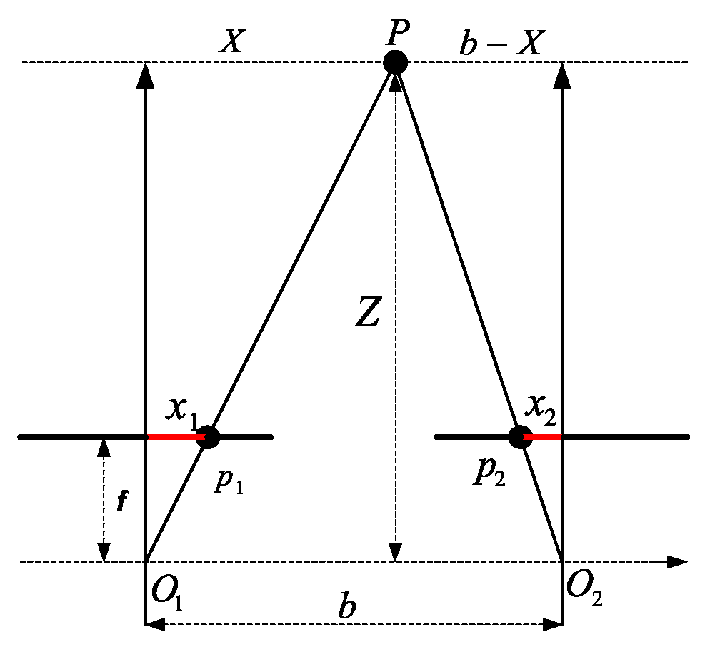
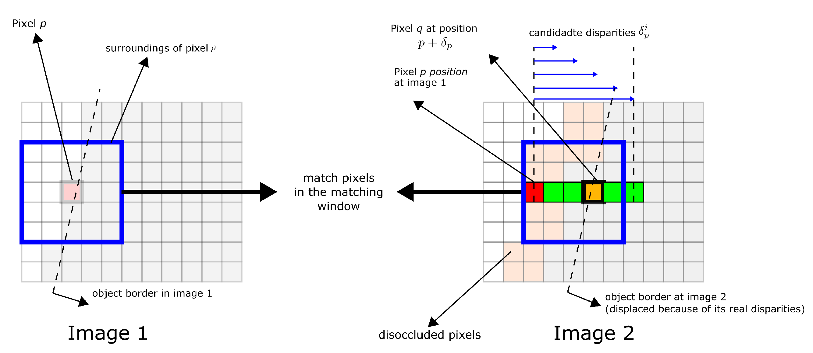
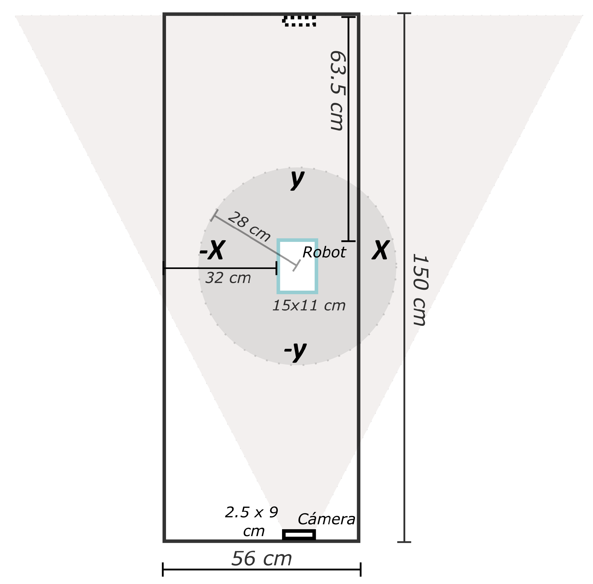
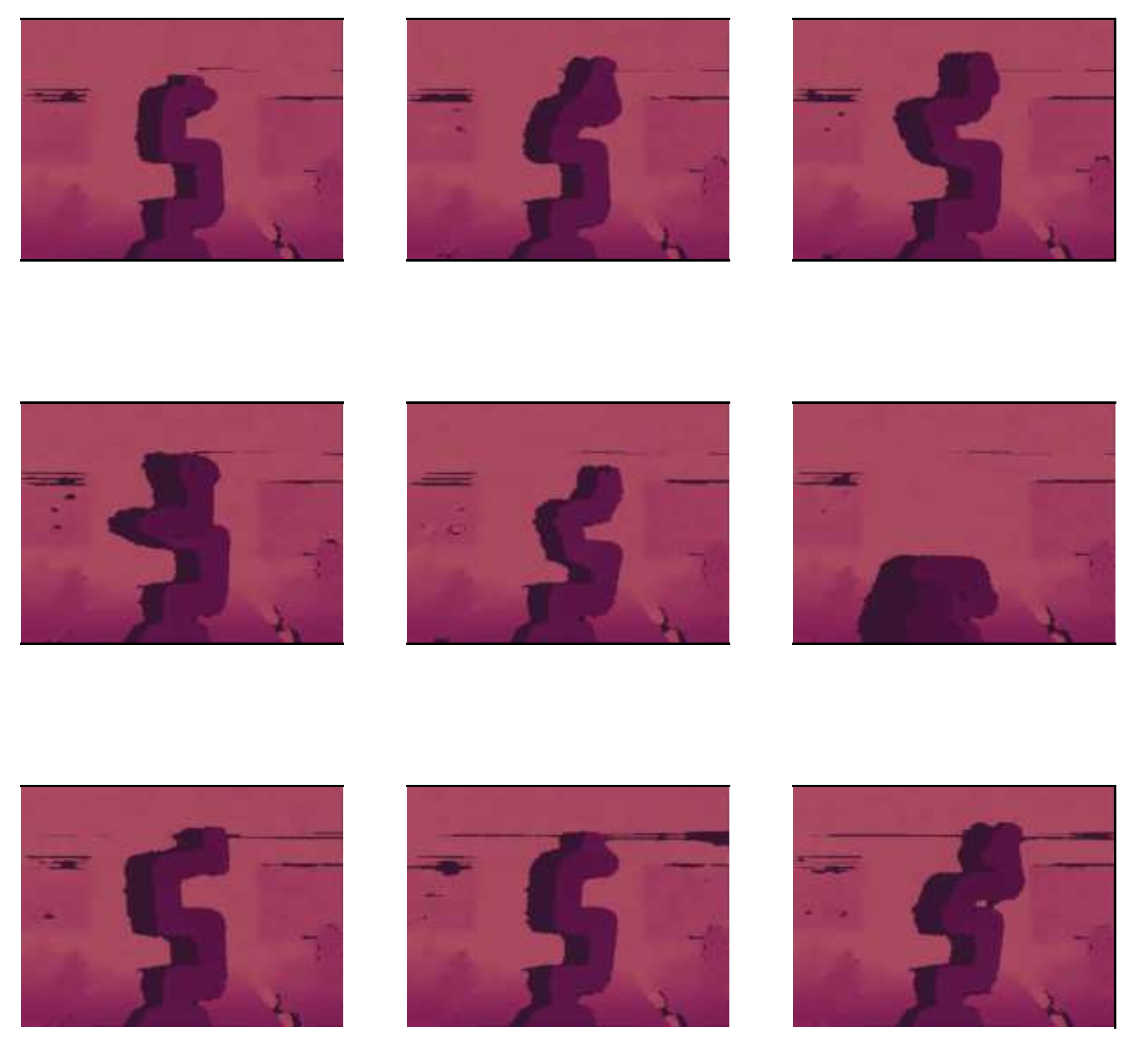
2.1. Stereo Vision
Accuracy of the D435 Stereo Camera
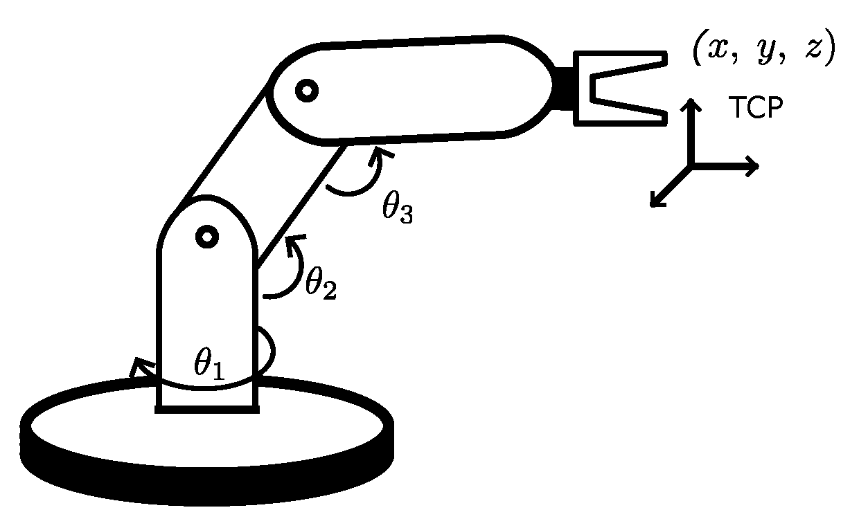
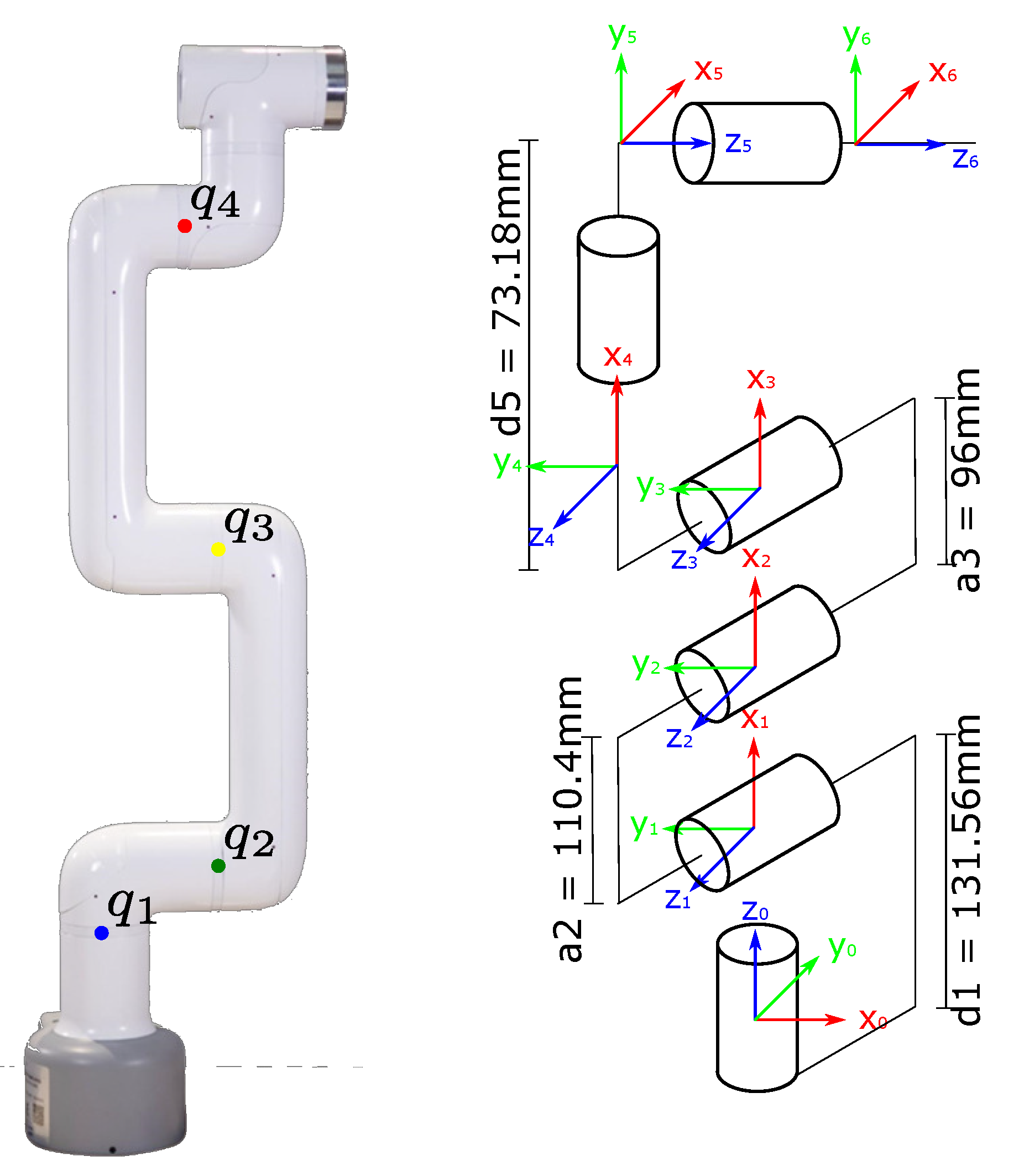
2.2. Materials
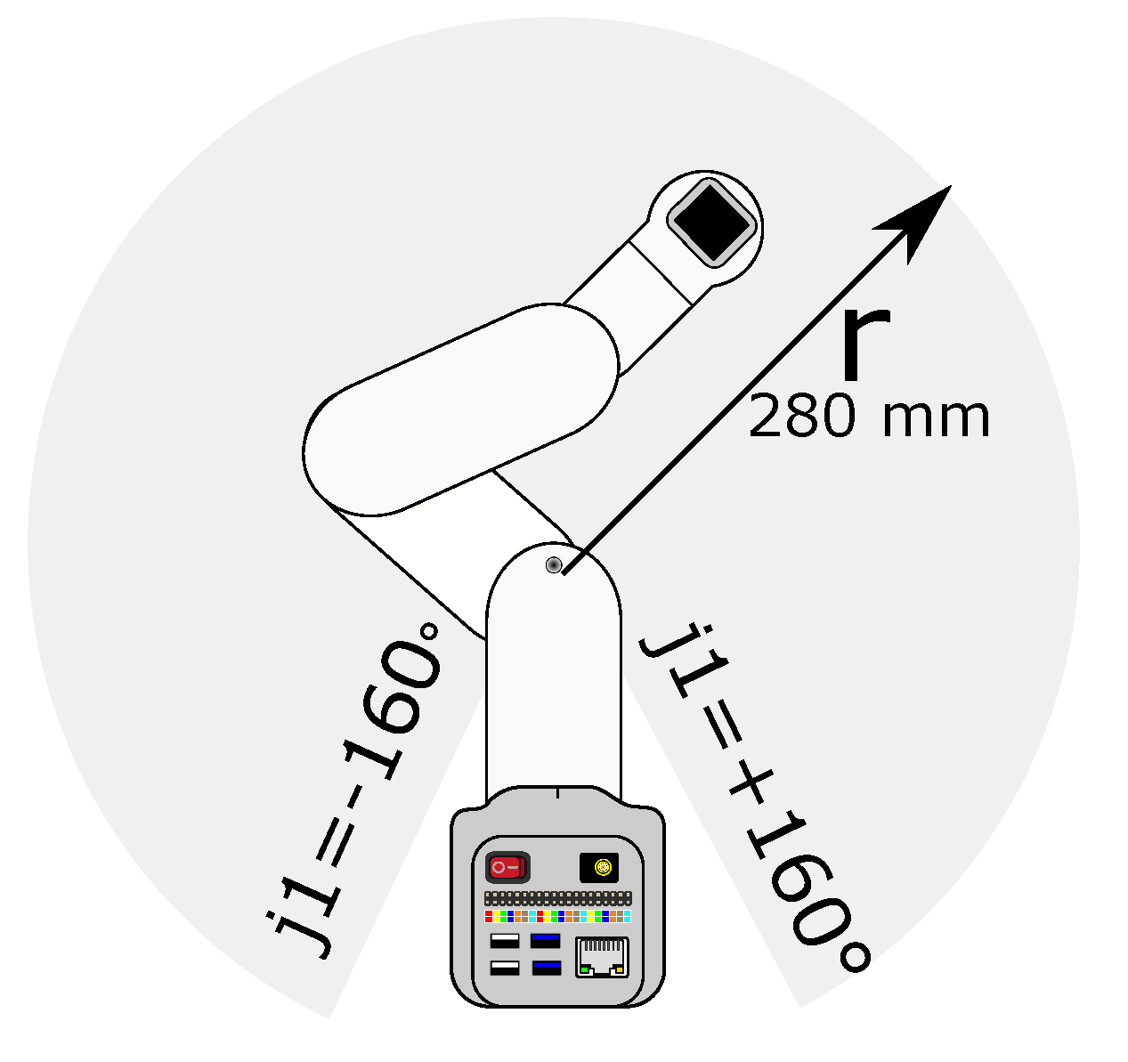
- 1 MyCobot 280 nano, its main features are:
- –
- Workspace 280 mm.
- –
- Joint range .
- –
- Repetitively mm.
- –
- A micro-computer Jetson nano 280, with 2 GB of RAM and NVIDIA processor
- –
- Servomotors of high precision.
- –
- 6 DoF.
- 1 depth camera model Intel RealSense D435. Its main features are:
- –
- Focal length of mm.
- –
- Depth resolution pixels, mm
- –
- Workspace –10 m.
- –
- 6 DoF para calibración.
- A generic monitor.
- Mouse and keyboard.
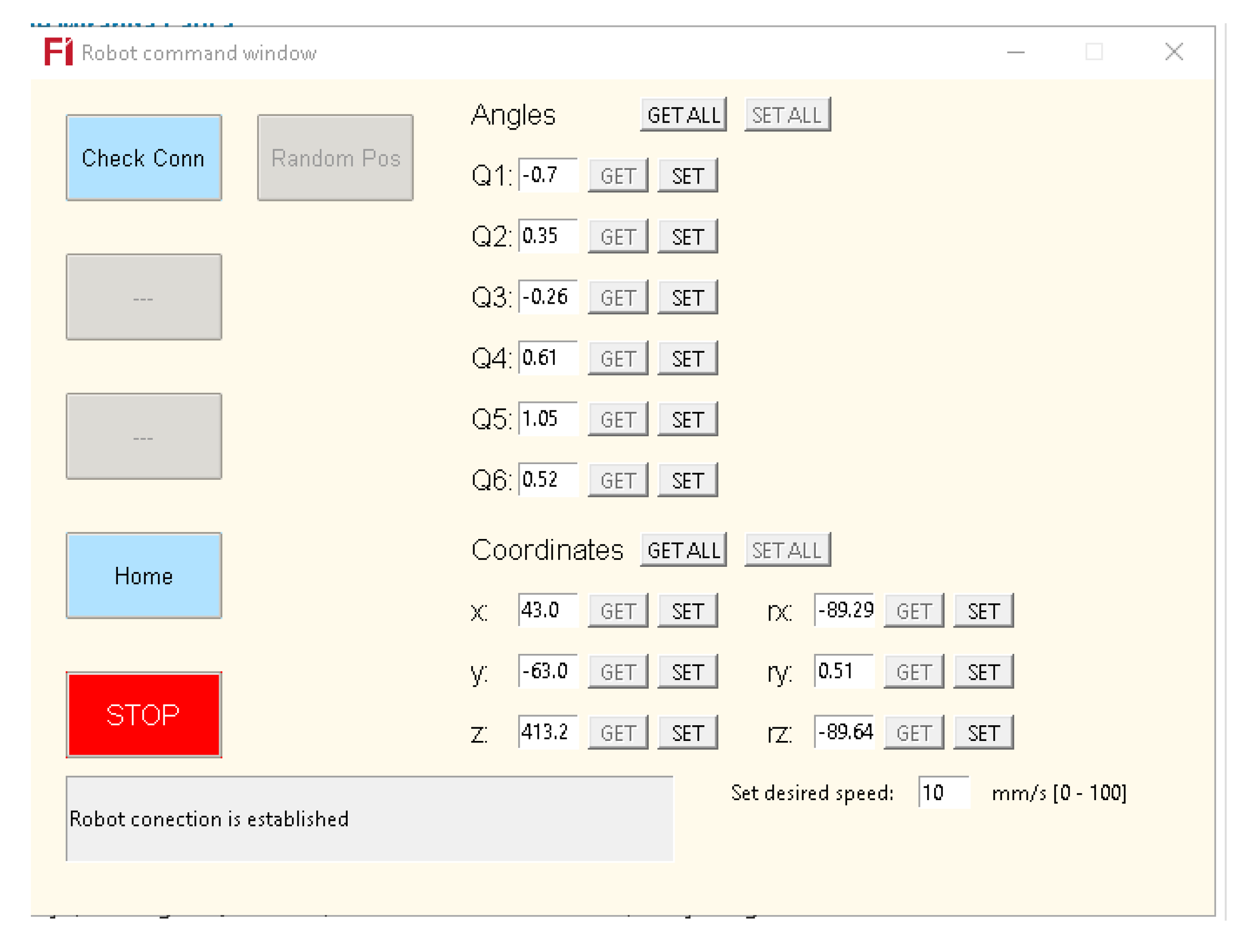
2.3. Graphical User Interface (GUI)
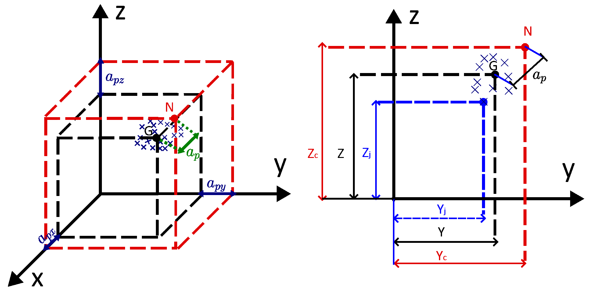
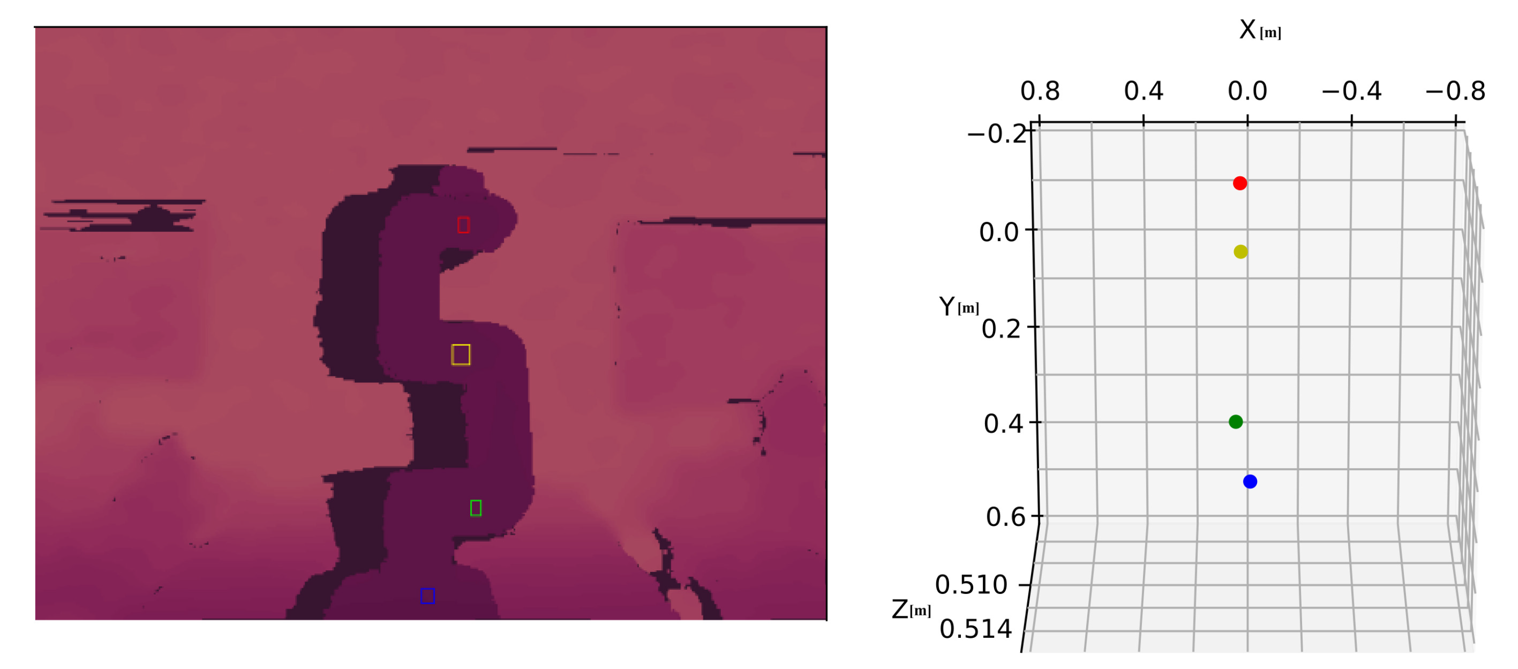
2.4. Measurement of Position Accuracy
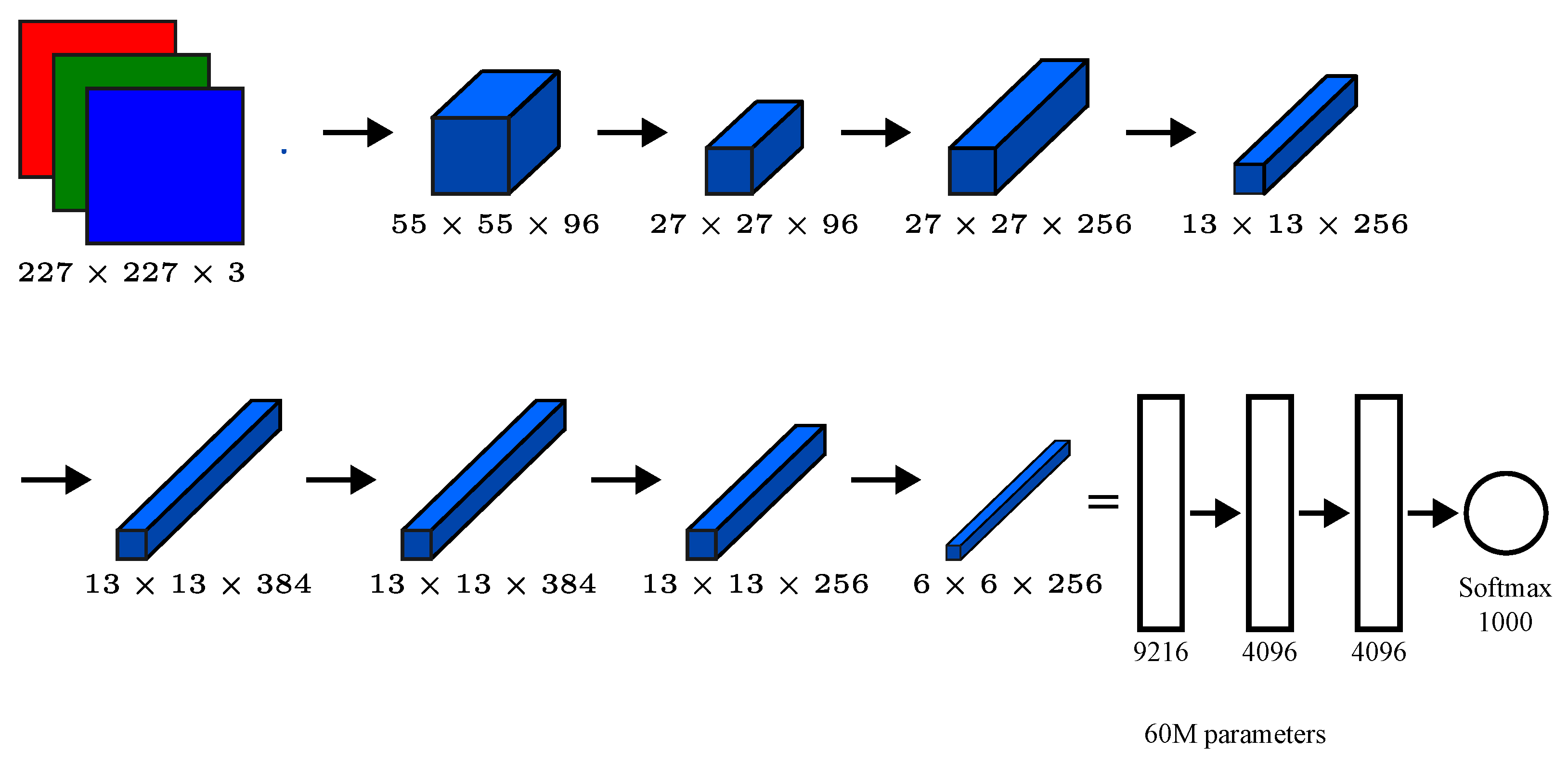
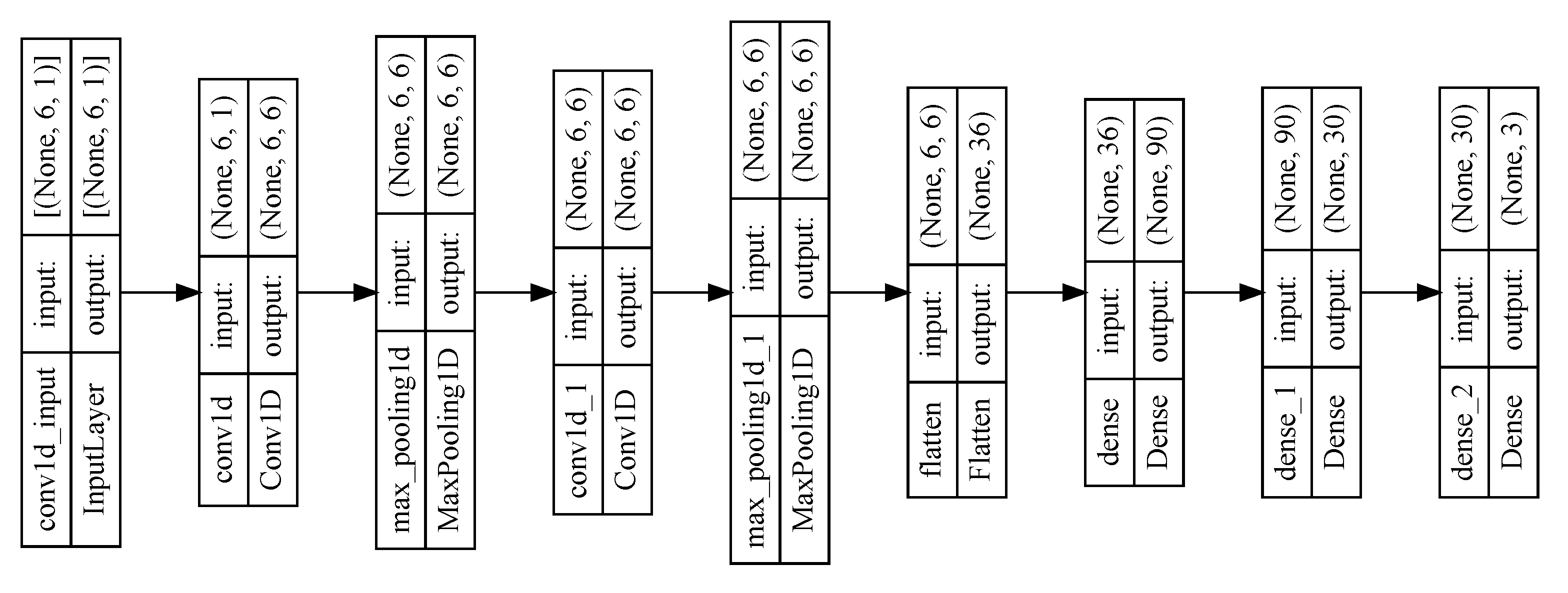
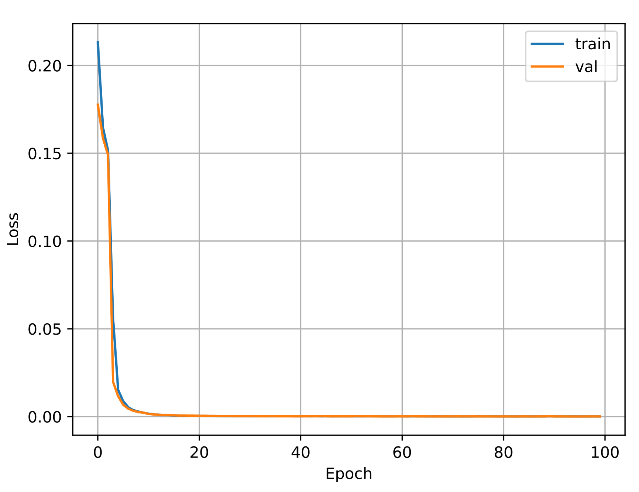
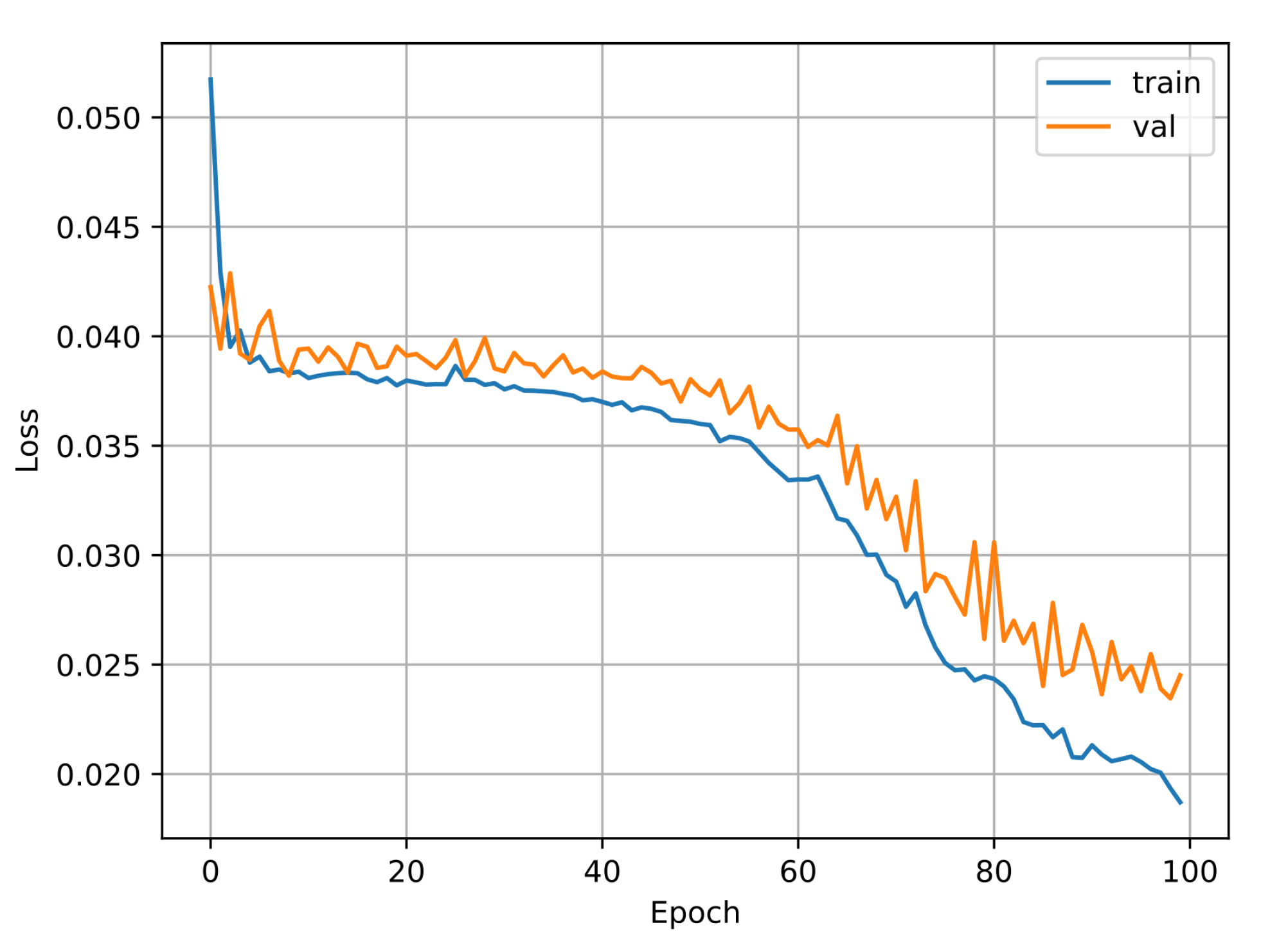
2.5. Convolutional Neural Networks
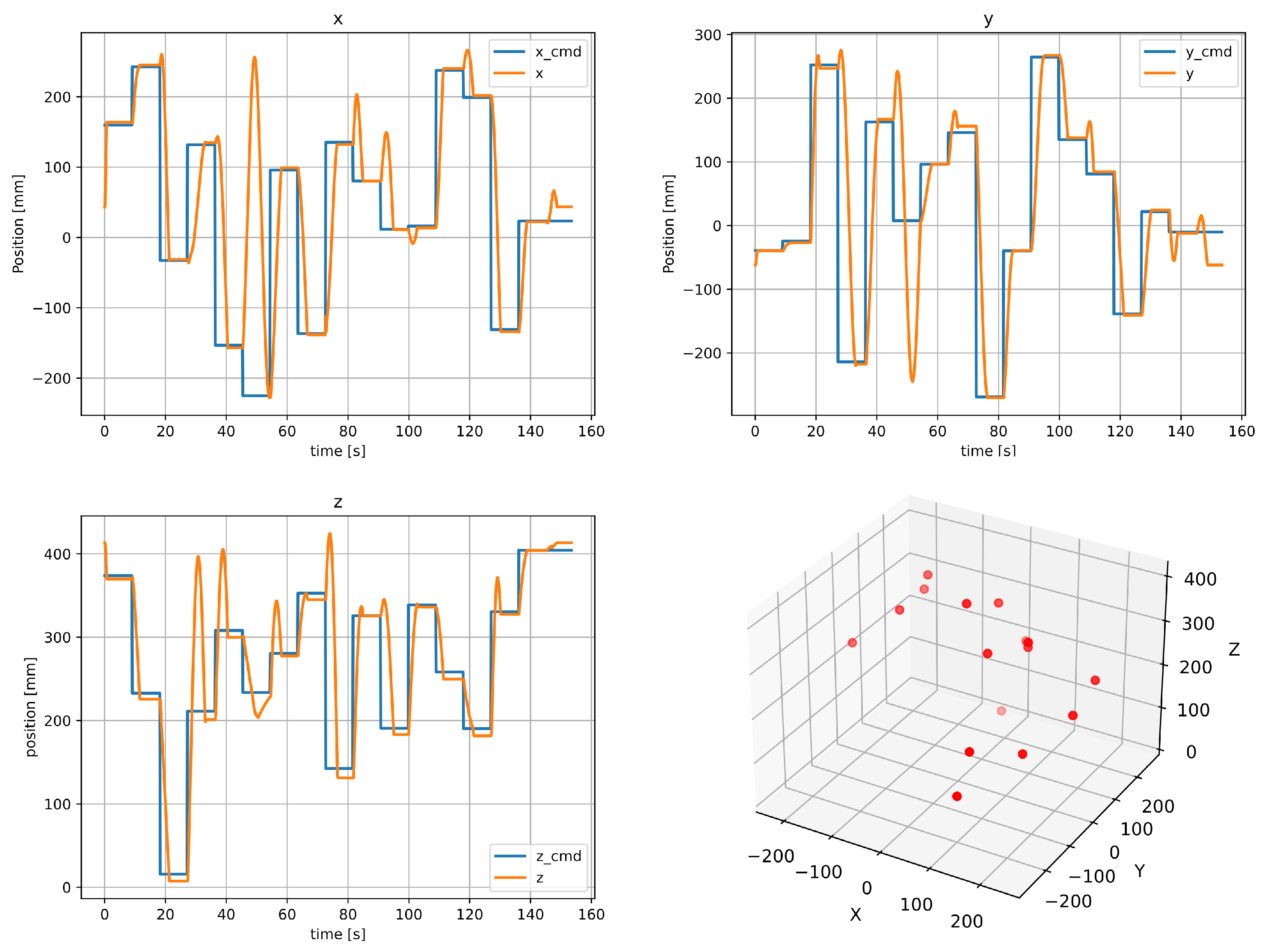
3. Results
4. Discussion
5. Conclusions
Author Contributions
Funding
Institutional Review Board Statement
Data Availability Statement
Acknowledgments
Conflicts of Interest
References
- Kelly, R.; Santibáñez, V. Control de Movimiento de Robots Manipuladores; Pearson Educación: London, UK, 2003. [Google Scholar]
- Qiao, G.; Weiss, B. Industrial robot accuracy degradation monitoring and quick health assessment. J. Manuf. Sci. Eng. 2019, 141, 071006. [Google Scholar] [CrossRef]
- Zhang, D.; Peng, Z.; Ning, G.; Han, X. Positioning accuracy reliability of industrial robots through probability and evidence theories. J. Mech. Des. 2021, 143, 011704. [Google Scholar] [CrossRef]
- Wang, Z.; Liu, R.; Sparks, T.; Chen, X.; Liou, F. Industrial Robot Trajectory Accuracy Evaluation Maps for Hybrid Manufacturing Process Based on Joint Angle Error Analysis; OMICS International: Hyderabad, India, 2018. [Google Scholar]
- Pérez, L.; Rodrıíguez, Í.; Rodríguez, N.; Usamentiaga, R.; García, D. Robot guidance using machine vision techniques in industrial environments: A comparative review. Sensors 2016, 16, 335. [Google Scholar] [CrossRef]
- Corke, P. Robotics, Vision and Control: Fundamental Algorithms in MATLAB® Second, Completely Revised; Springer: Berlin/Heidelberg, Germany, 2017. [Google Scholar]
- Zeng, R.; Liu, M.; Zhang, J.; Li, X.; Zhou, Q.; Jiang, Y. Manipulator control method based on deep reinforcement learning. In Proceedings of the 2020 Chinese Control And Decision Conference (CCDC), Hefei, China, 22–24 August 2020; pp. 415–420. [Google Scholar]
- Sangeetha, G.; Kumar, N.; Hari, P.; Sasikumar, S. Implementation of a stereo vision based system for visual feedback control of robotic arm for space manipulations. Procedia Comput. Sci. 2018, 133, 1066–1073. [Google Scholar]
- Liang, B.; Li, T.; Chen, Z.; Wang, Y.; Liao, Y. Robot arm dynamics control based on deep learning and physical simulation. In Proceedings of the 2018 37th Chinese Control Conference (CCC), Wuhan, China, 25–27 July 2018; pp. 2921–2925. [Google Scholar]
- Li, C.; Chang, Y. Automated visual positioning and precision placement of a workpiece using deep learning. Int. J. Adv. Manuf. Technol. 2019, 104, 4527–4538. [Google Scholar] [CrossRef]
- Li, Q.; Pang, Y.; Wang, Y.; Han, X.; Li, Q.; Zhao, M. CBMC: A Biomimetic Approach for Control of a 7-Degree of Freedom Robotic Arm. Biomimetics 2023, 8, 389. [Google Scholar] [CrossRef] [PubMed]
- Athulya, P.; George, N. Others A Computer Vision Approach for the Inverse Kinematics of 2 DOF Manipulators Using Neural Network. In Proceedings of the 2020 IEEE Recent Advances In Intelligent Computational Systems (RAICS), Thiruvananthapuram, India, 3–5 December 2020; pp. 80–85. [Google Scholar]
- Cavalcanti, S.; Santana, O. Self-learning in the inverse kinematics of robotic arm. In Proceedings of the 2017 Latin American Robotics Symposium (LARS) and 2017 Brazilian Symposium on Robotics (SBR), Curitiba, Brazil, 8–11 November 2017; pp. 1–5. [Google Scholar]
- Wang, C.; Wang, C.; Li, W.; Wang, H. A brief survey on RGB-D semantic segmentation using deep learning. Displays 2021, 70, 102080. [Google Scholar] [CrossRef]
- Wu, Z.; Allibert, G.; Stolz, C.; Ma, C.; Demonceaux, C. Depth-adapted CNNs for RGB-D semantic segmentation. arXiv 2022, arXiv:2206.03939. [Google Scholar]
- Du, Y.; Muslikhin, M.; Hsieh, T.; Wang, M. Stereo vision-based object recognition and manipulation by regions with convolutional neural network. Electronics 2020, 9, 210. [Google Scholar] [CrossRef]
- Halmetschlager-Funek, G.; Suchi, M.; Kampel, M.; Vincze, M. An empirical evaluation of ten depth cameras: Bias, precision, lateral noise, different lighting conditions and materials, and multiple sensor setups in indoor environments. IEEE Robot. Autom. Mag. 2018, 26, 67–77. [Google Scholar] [CrossRef]
- Fischer, M.; Mylo, M.; Lorenz, L.; Böckenholt, L.; Beismann, H. Stereo Camera Setup for 360° Digital Image Correlation to Reveal Smart Structures of Hakea Fruits. Biomimetics 2024, 9, 191. [Google Scholar] [CrossRef] [PubMed]
- Priorelli, M.; Pezzulo, G.; Stoianov, I. Active Vision in Binocular Depth Estimation: A Top-Down Perspective. Biomimetics 2023, 8, 445. [Google Scholar] [CrossRef] [PubMed]
- Zhang, H.; Lee, S. Advancing the Robotic Vision Revolution: Development and Evaluation of a Bionic Binocular System for Enhanced Robotic Vision. Biomimetics 2024, 9, 371. [Google Scholar] [CrossRef] [PubMed]
- Pérez, R.; Gutiérrez, S.; Zotovic, R. A study on robot arm machining: Advance and future challenges. Ann. Daaam Proc. 2018, 29, 0931. [Google Scholar]
- Wang, T.; Tao, Y.; Liu, H. Current researches and future development trend of intelligent robot: A review. Int. J. Autom. Comput. 2018, 15, 525–546. [Google Scholar] [CrossRef]
- Wu, J.; Zhang, D.; Liu, J.; Han, X. A moment approach to positioning accuracy reliability analysis for industrial robots. IEEE Trans. Reliab. 2019, 69, 699–714. [Google Scholar] [CrossRef]
- Hsiao, J.; Shivam, K.; Lu, I.; Kam, T. Positioning accuracy improvement of industrial robots considering configuration and payload effects via a hybrid calibration approach. IEEE Access 2020, 8, 228992–229005. [Google Scholar] [CrossRef]
- Jiang, Y.; Yu, L.; Jia, H.; Zhao, H.; Xia, H. Absolute positioning accuracy improvement in an industrial robot. Sensors 2020, 20, 4354. [Google Scholar] [CrossRef]
- Lee, T.; Tremblay, J.; To, T.; Cheng, J.; Mosier, T.; Kroemer, O.; Fox, D.; Birchfield, S. Camera-to-robot pose estimation from a single image. In Proceedings of the 2020 IEEE International Conference on Robotics and Automation (ICRA), Paris, France, 31 May–31 August 2020; pp. 9426–9432. [Google Scholar]
- Abdelaal, M.; Farag, R.; Saad, M.; Bahgat, A.; Emara, H.; El-Dessouki, A. Uncalibrated stereo vision with deep learning for 6-DOF pose estimation for a robot arm system. Robot. Auton. Syst. 2021, 145, 103847. [Google Scholar] [CrossRef]
- Chen, T.; Lin, J.; Wu, D.; Wu, H. Research of calibration method for industrial robot based on error model of position. Appl. Sci. 2021, 11, 1287. [Google Scholar] [CrossRef]
- Sellami, S.; Klimchik, A. A deep learning based robot positioning error compensation. In Proceedings of the 2021 International Conference “Nonlinearity, Information and Robotics” (NIR), Innopolis, Russia, 26–29 August 2021; pp. 1–5. [Google Scholar]
- Galan-Uribe, E.; Morales-Velazquez, L.; Osornio-Rios, R. FPGA-Based Methodology for Detecting Positional Accuracy Degradation in Industrial Robots. Appl. Sci. 2023, 13, 8493. [Google Scholar] [CrossRef]
- Galan-Uribe, E.; Amezquita-Sanchez, J.; Morales-Velazquez, L. Supervised Machine-Learning Methodology for Industrial Robot Positional Health Using Artificial Neural Networks, Discrete Wavelet Transform, and Nonlinear Indicators. Sensors 2023, 23, 3213. [Google Scholar] [CrossRef] [PubMed]
- Khanafer, M.; Shirmohammadi, S. Applied AI in instrumentation and measurement: The deep learning revolution. IEEE Instrum. Meas. Mag. 2020, 23, 10–17. [Google Scholar] [CrossRef]
- Chellappa, R.; Theodoridis, S. Academic Press Library in Signal Processing, Volume 6: Image and Video Processing and Analysis and Computer Vision; Academic Press: Cambridge, MA, USA, 2017. [Google Scholar]
- ISO 9283:1998; International Organization for Standardization Manipulating Industrial Robots—Performance Criteria and Related Test Methods. ISO: Geneva, Switzerland, 1998.
- LeCun, Y.; Bottou, L.; Bengio, Y.; Haffner, P. Gradient-based learning applied to document recognition. Proc. IEEE. 1998, 86, 2278–2324. [Google Scholar] [CrossRef]
- Krizhevsky, A.; Sutskever, I.; Hinton, G. Imagenet classification with deep convolutional neural networks. Adv. Neural Inf. Process. Syst. 2012, 25, 84–90. [Google Scholar] [CrossRef]
- Redmon, J.; Divvala, S.; Girshick, R.; Farhadi, A. You only look once: Unified, real-time object detection. In Proceedings of the IEEE Conference on Computer Vision and Pattern Recognition, Las Vegas, NV, USA, 27–30 June 2016; pp. 779–788. [Google Scholar]


| Reference | Conventional Techniques | AI Techniques | Robotic Vision | ME before [mm] | ME after [mm] |
|---|---|---|---|---|---|
| [23] | ✓ | ||||
| [24] | ✓ | ✓ | 2.613 | 0.31 | |
| [25] | ✓ | ✓ | 0.7411 | 0.1007 | |
| [26] | ✓ | ✓ | 27.4 | ||
| [27] | ✓ | ✓ | |||
| [28] | ✓ | 1.2248 | 0.2678 | ||
| [29] | ✓ | ✓ | 0.1 | ||
| [30] | ✓ | ✓ | |||
| [31] | ✓ | ✓ |
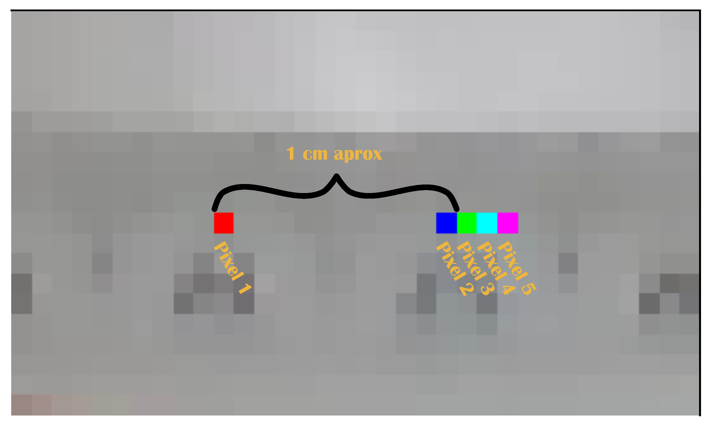
| Pixels | Distance [mm] |
|---|---|
| 1 to 2 | 13.9 |
| 1 to 3 | 15.0 |
| 1 to 4 | 16.3 |
| 1 to 5 | 17.7 |
| Pixels | Distance between Two Consecutive Pixels [mm] |
|---|---|
| 3–2 | 1.1 |
| 4–3 | 1.3 |
| 5–4 | 1.4 |
Disclaimer/Publisher’s Note: The statements, opinions and data contained in all publications are solely those of the individual author(s) and contributor(s) and not of MDPI and/or the editor(s). MDPI and/or the editor(s) disclaim responsibility for any injury to people or property resulting from any ideas, methods, instructions or products referred to in the content. |
© 2024 by the authors. Licensee MDPI, Basel, Switzerland. This article is an open access article distributed under the terms and conditions of the Creative Commons Attribution (CC BY) license (https://creativecommons.org/licenses/by/4.0/).
Share and Cite
Cabrera-Rufino, M.-A.; Ramos-Arreguín, J.-M.; Aceves-Fernandez, M.-A.; Gorrostieta-Hurtado, E.; Pedraza-Ortega, J.-C.; Rodríguez-Resendiz, J. Pose Estimation of a Cobot Implemented on a Small AI-Powered Computing System and a Stereo Camera for Precision Evaluation. Biomimetics 2024, 9, 610. https://doi.org/10.3390/biomimetics9100610
Cabrera-Rufino M-A, Ramos-Arreguín J-M, Aceves-Fernandez M-A, Gorrostieta-Hurtado E, Pedraza-Ortega J-C, Rodríguez-Resendiz J. Pose Estimation of a Cobot Implemented on a Small AI-Powered Computing System and a Stereo Camera for Precision Evaluation. Biomimetics. 2024; 9(10):610. https://doi.org/10.3390/biomimetics9100610
Chicago/Turabian StyleCabrera-Rufino, Marco-Antonio, Juan-Manuel Ramos-Arreguín, Marco-Antonio Aceves-Fernandez, Efren Gorrostieta-Hurtado, Jesus-Carlos Pedraza-Ortega, and Juvenal Rodríguez-Resendiz. 2024. "Pose Estimation of a Cobot Implemented on a Small AI-Powered Computing System and a Stereo Camera for Precision Evaluation" Biomimetics 9, no. 10: 610. https://doi.org/10.3390/biomimetics9100610