
Stability and Controller Research of Double-Wing FMAV System Based on Controllable Tail
 , , ,
, , ,
Abstract
:1. Introduction
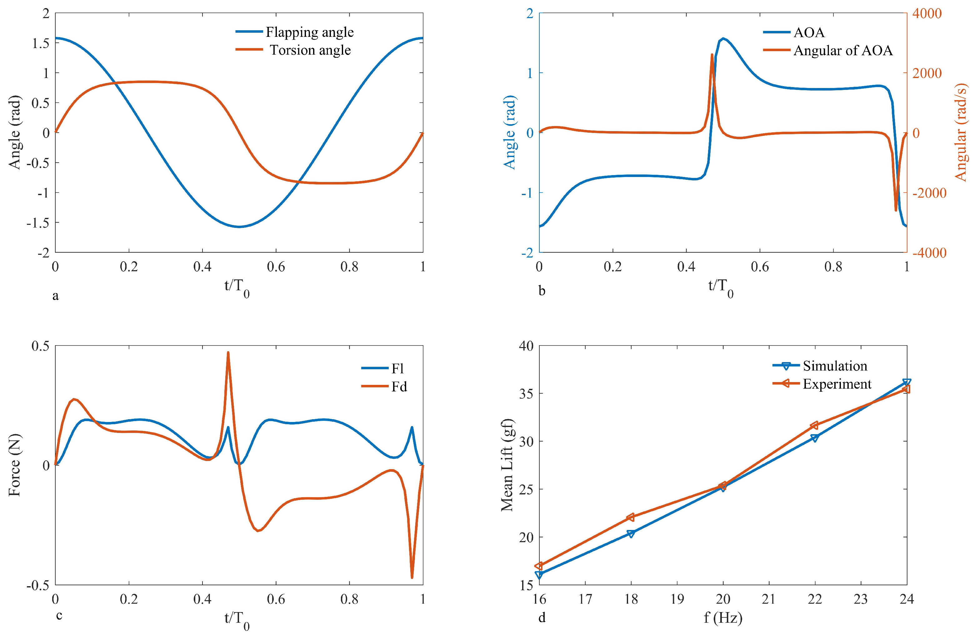
2. Flap Lift Model
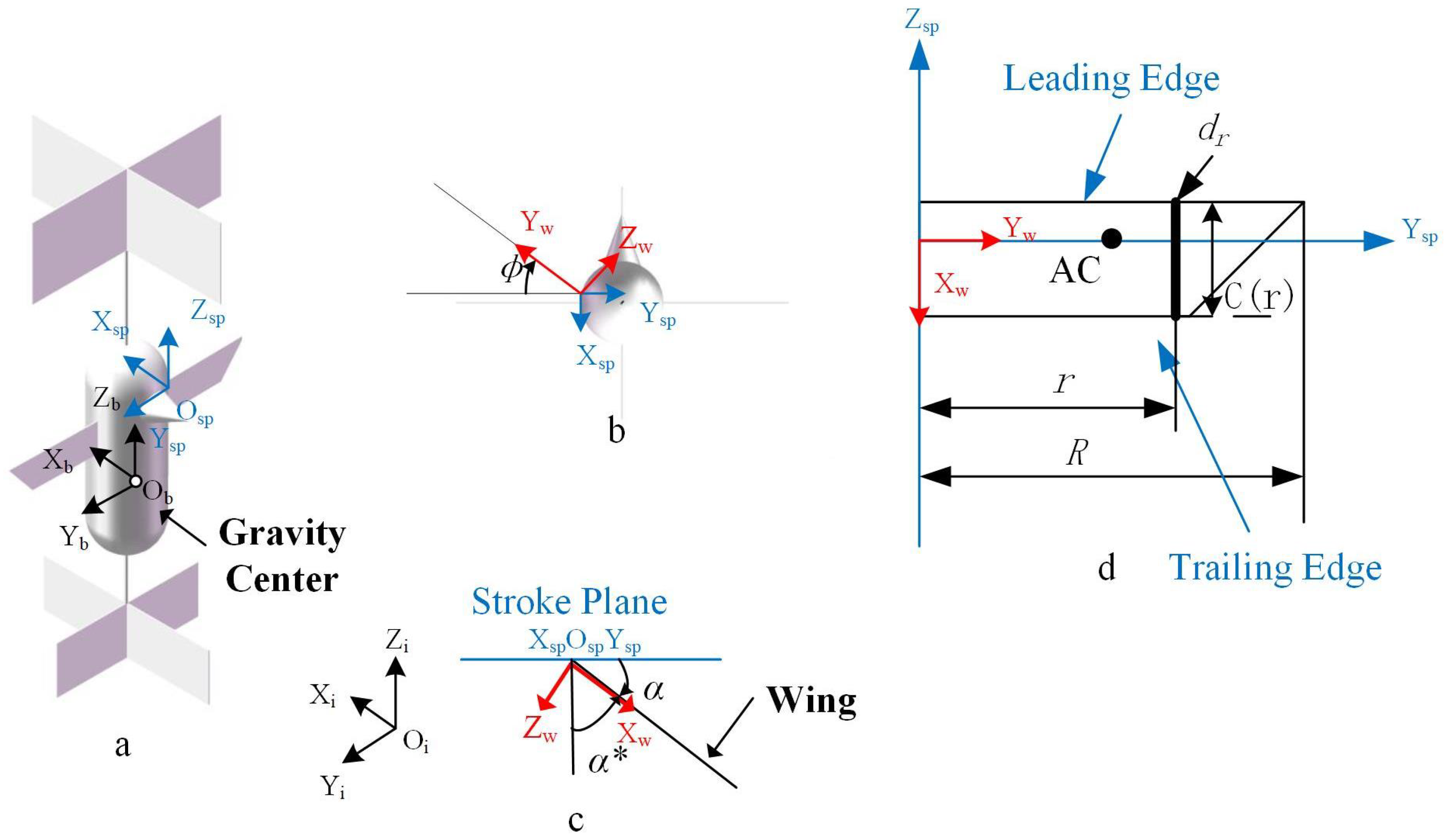
2.1. Description Movement
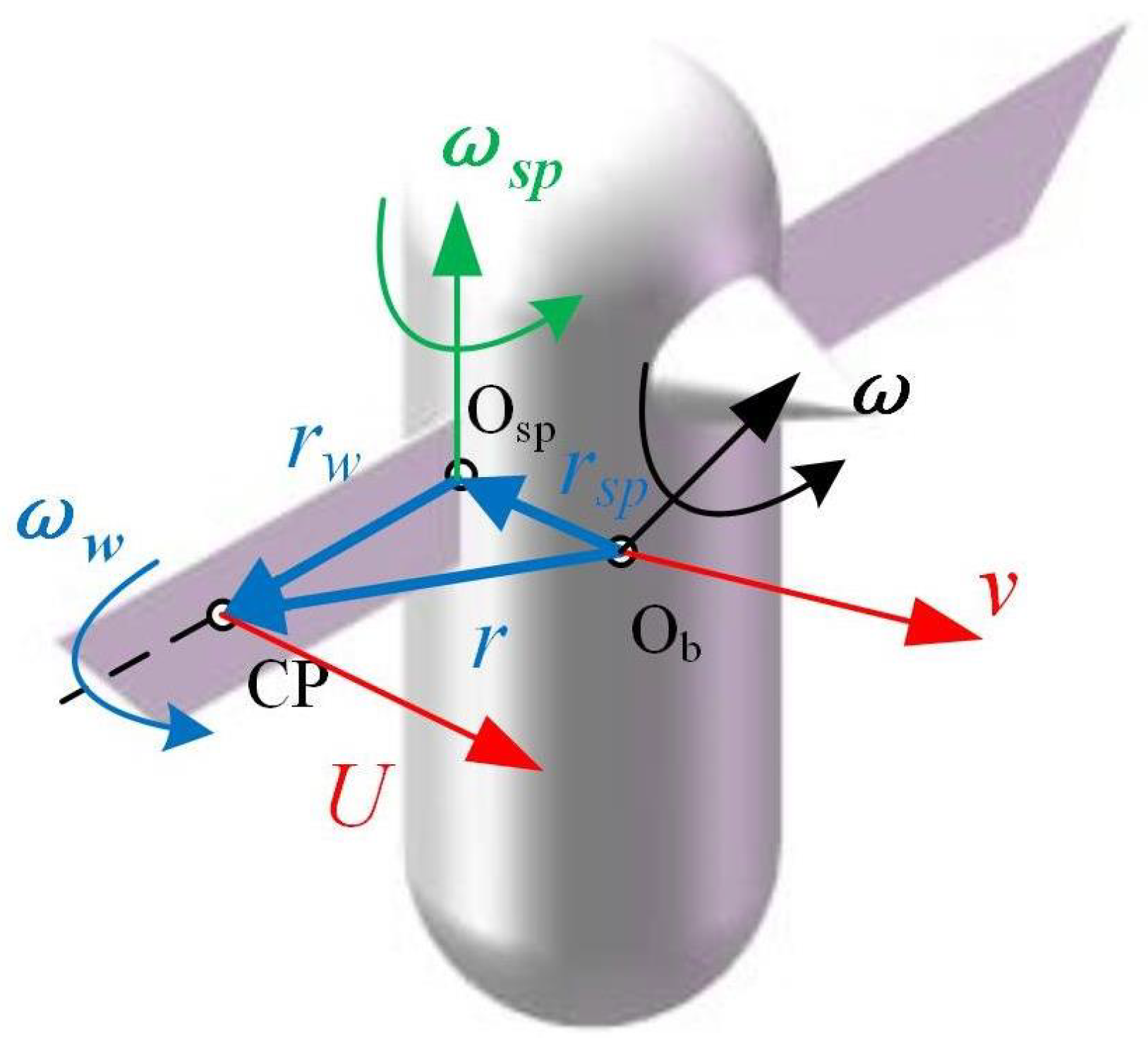
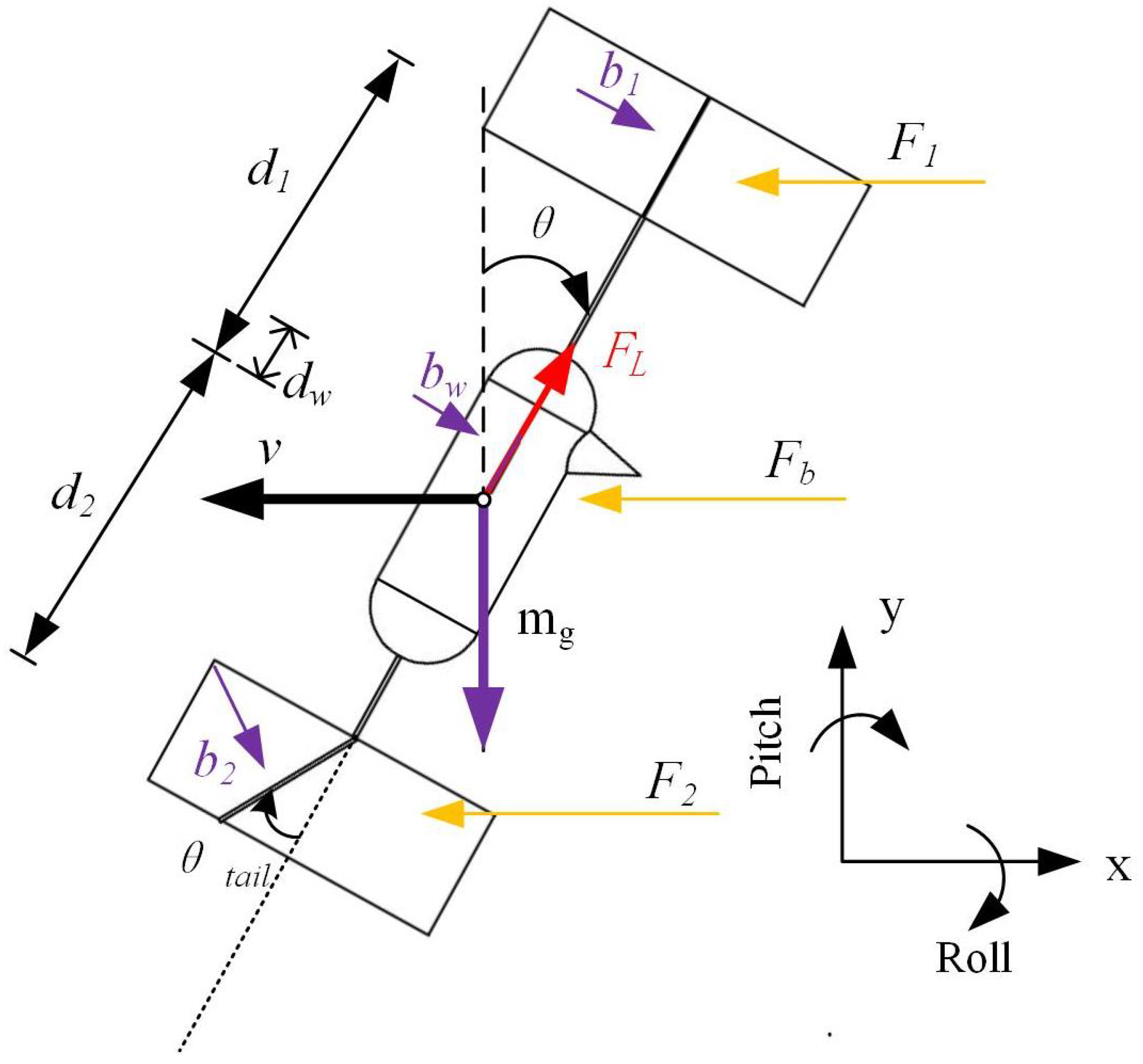
2.2. Description of Force
3. Tail Design and Torque Measurements
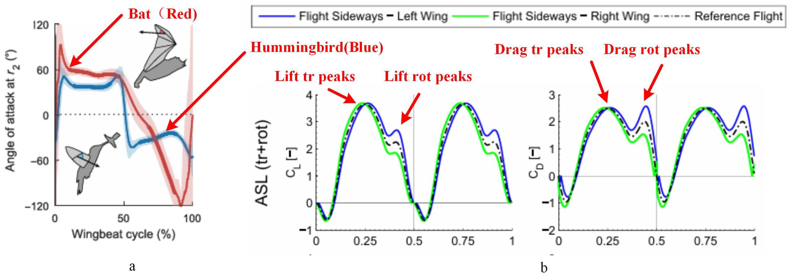
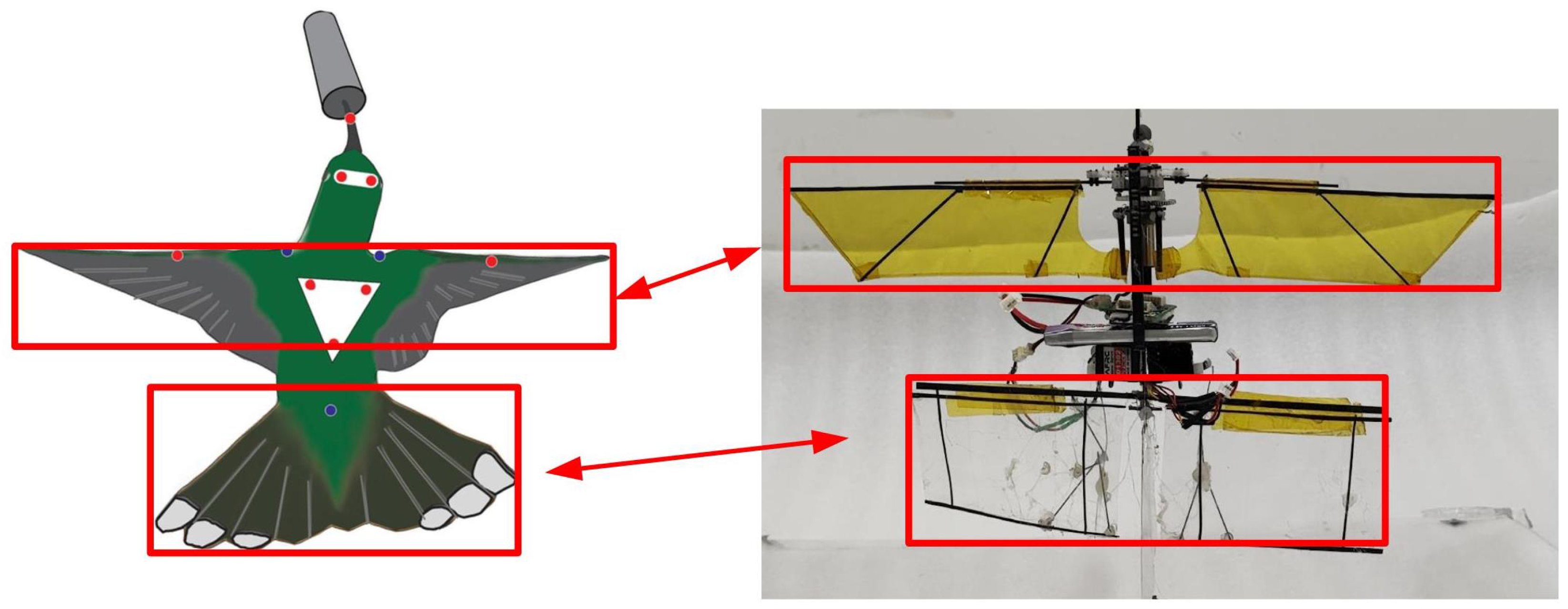
3.1. The Morphology of a Hummingbird’s Tail
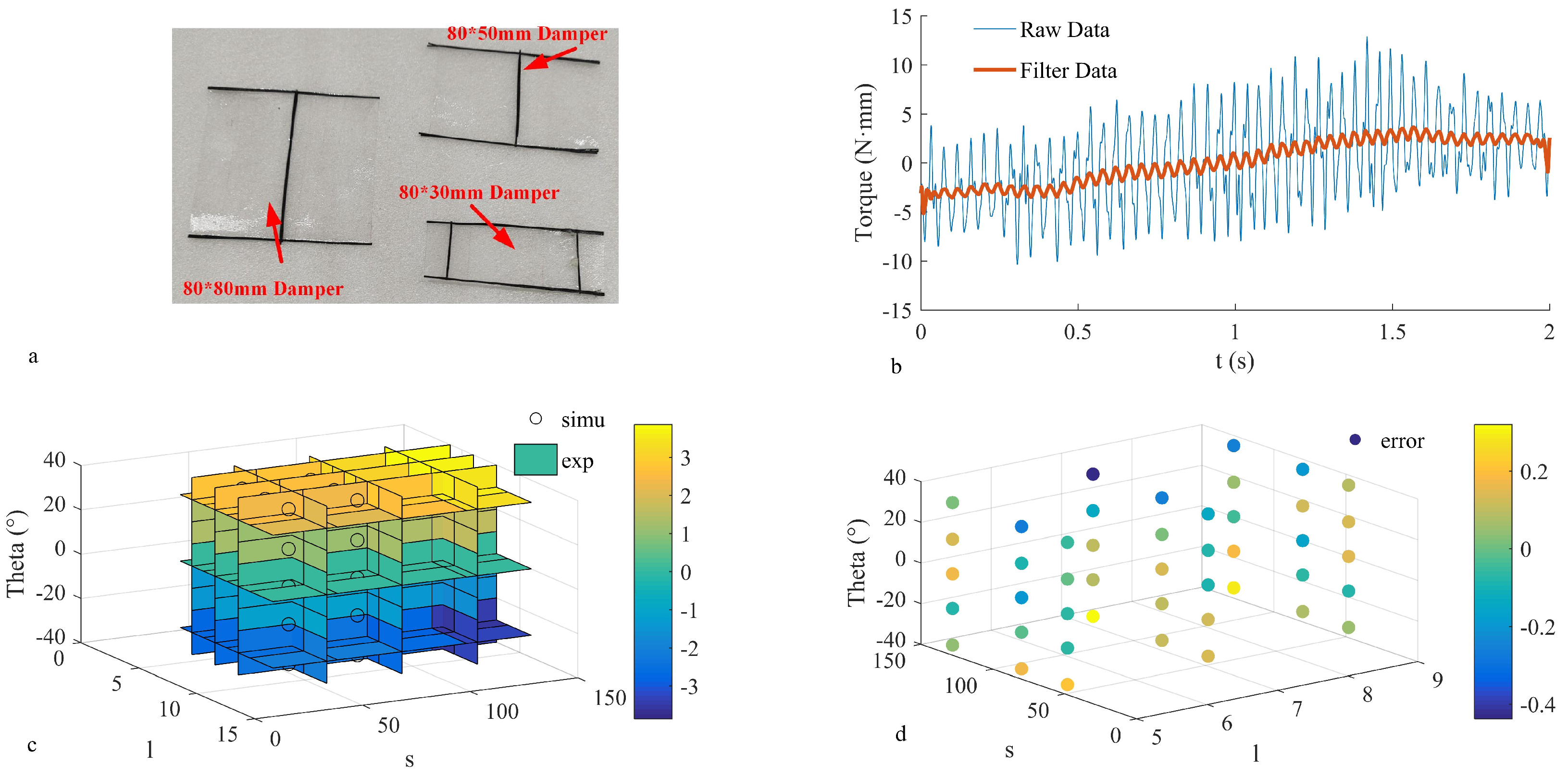
3.2. Tail Force Model and Measurements
4. FMAV Drag Model of Angle-Variable Tail
5. Simulation Model Controller Design
5.1. Analysis of Model Stability
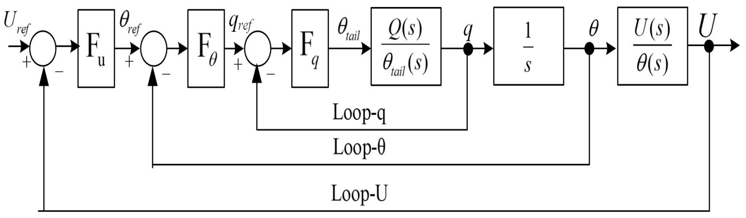
5.2. Series Simulation Controller Design
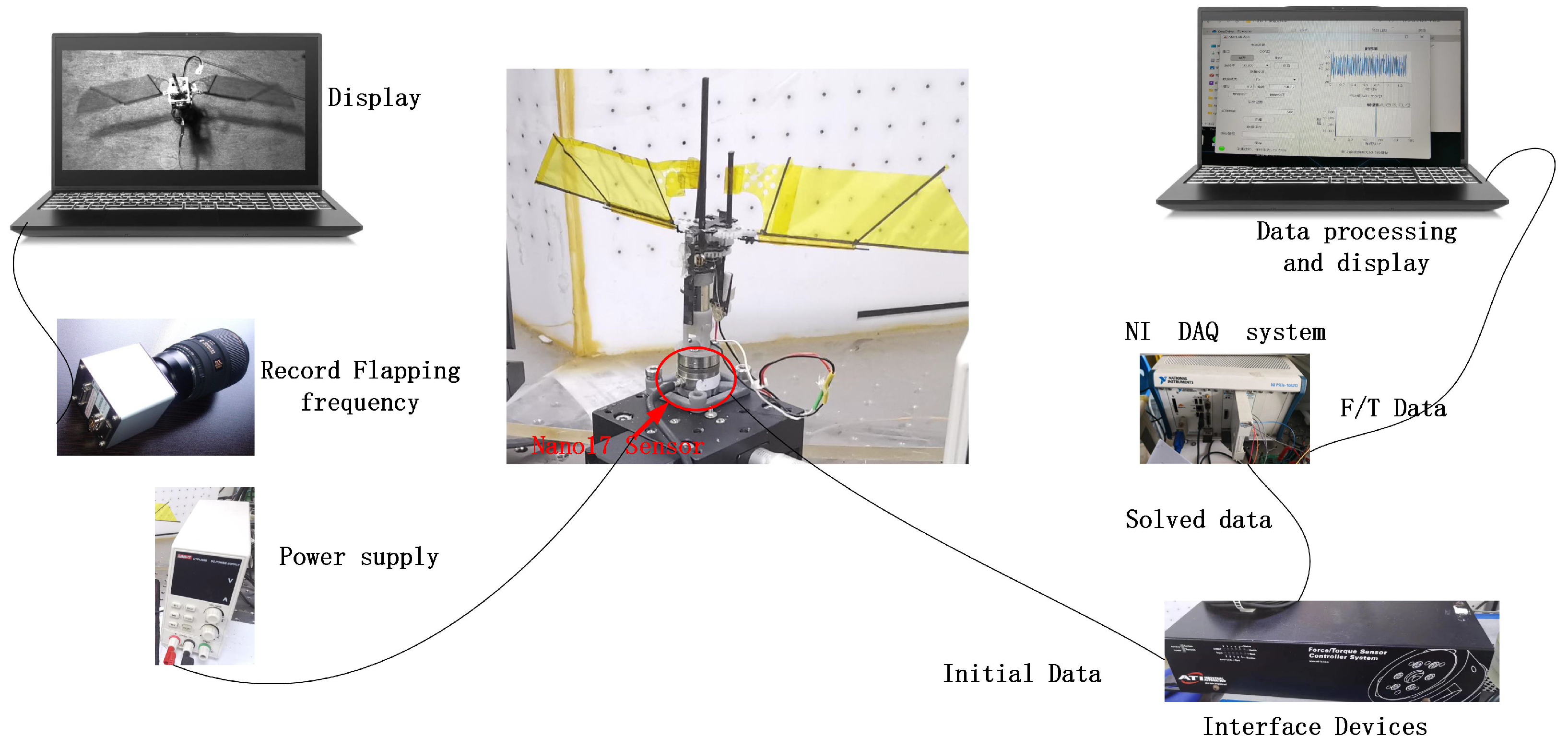
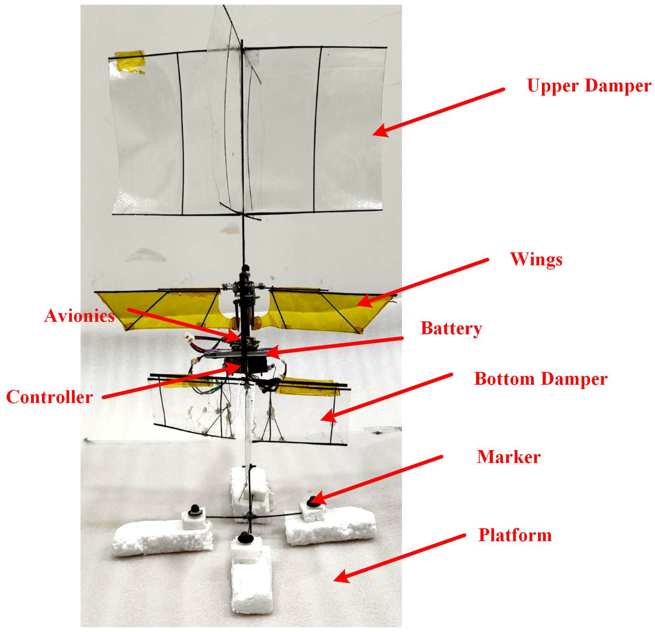
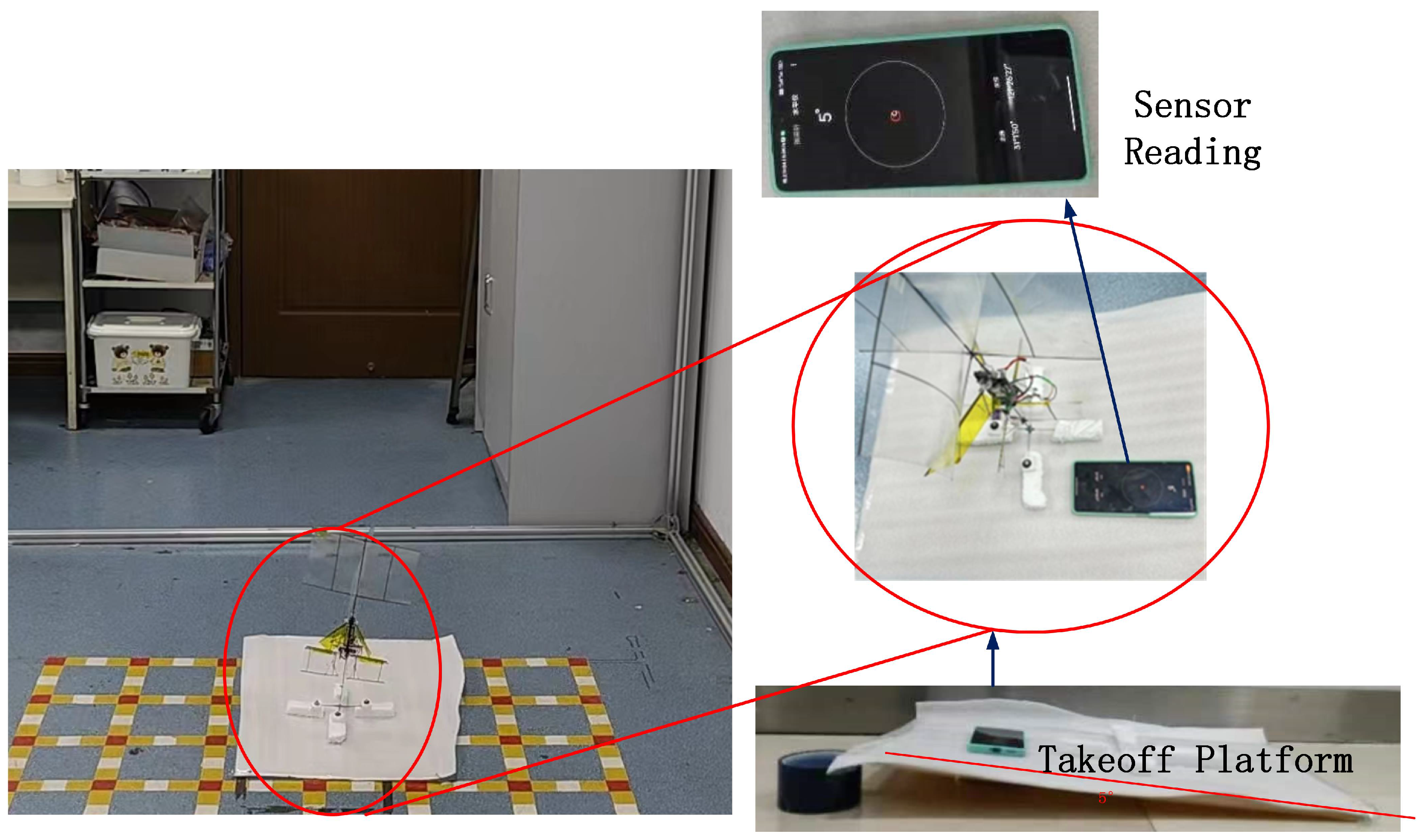
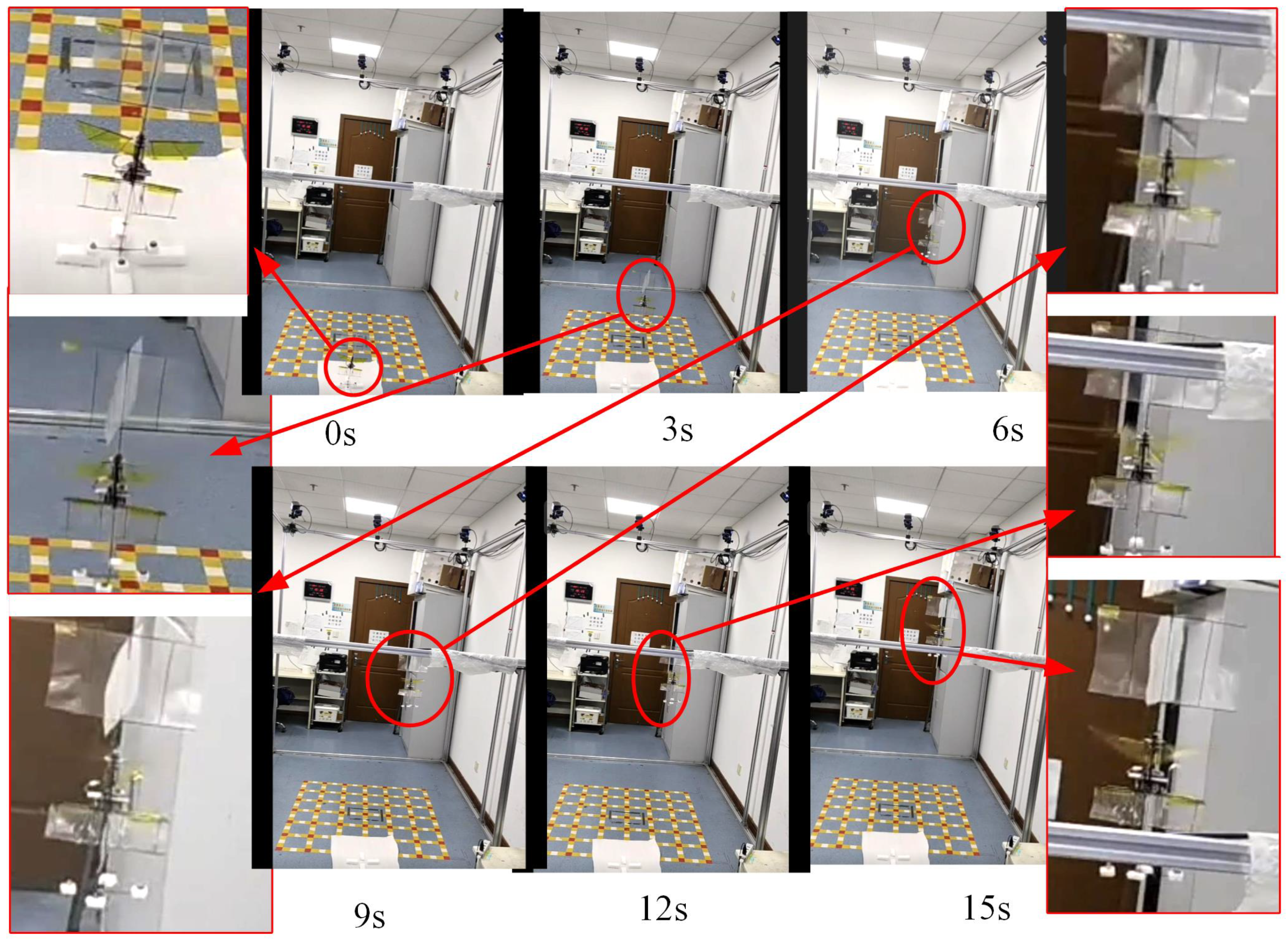
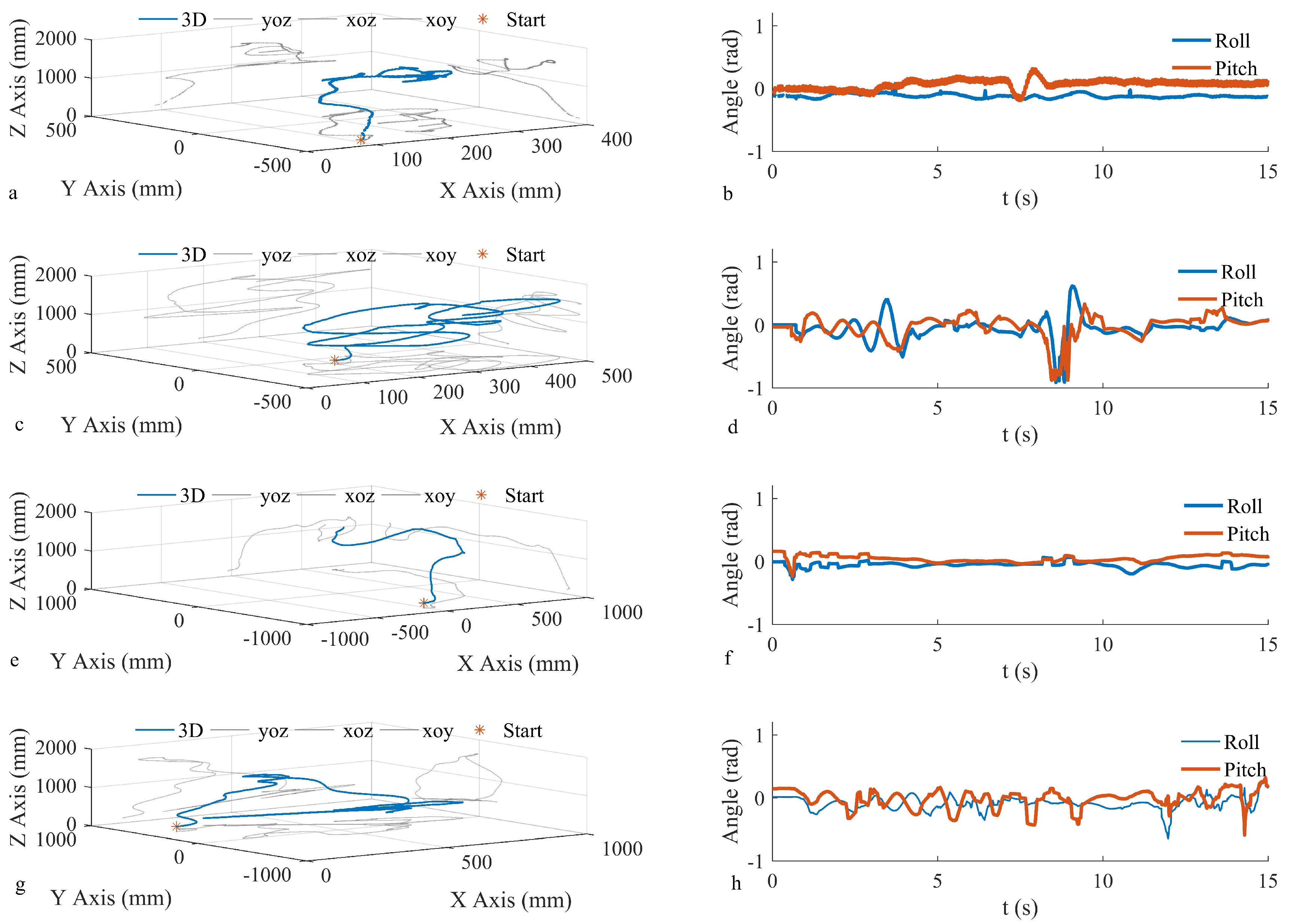
6. Physical Prototype Testing and Validation
7. Results
Supplementary Materials
Author Contributions
Funding
Institutional Review Board Statement
Informed Consent Statement
Data Availability Statement
Conflicts of Interest
Abbreviations
| FMAV | Flapping micro air vehicle |
| AOA | Angle of attack |
References
- Fei, F.; Tu, Z.; Zhang, J.; Deng, X. Learning extreme hummingbird maneuvers on flapping wing robots. In Proceedings of the 2019 International Conference on Robotics and Automation (ICRA), Montreal, QC, Canada, 20–24 May 2019; pp. 109–115. [Google Scholar]
- Hassanalian, M.; Abdelkefi, A. Classifications, applications, and design challenges of drones: A review. Prog. Aerosp. Sci. 2017, 91, 99–131. [Google Scholar] [CrossRef]
- Phan, H.V.; Park, H.C. Insect-inspired, tailless, hover-capable flapping-wing robots: Recent progress, challenges, and future directions. Prog. Aerosp. Sci. 2019, 111, 100573. [Google Scholar] [CrossRef]
- Phan, H.V.; Aurecianus, S.; Kang, T.; Park, H.C. Kubeetle-s: An insect-like, tailless, hover-capable robot that can fly with a low-torque control mechanism. Int. J. Micro Air Veh. 2019, 11, 1756829319861371. [Google Scholar] [CrossRef]
- Phan, H.V.; Park, H.C. Mechanisms of collision recovery in flying beetles and flapping-wing robots. Science 2020, 370, 1214–1219. [Google Scholar] [CrossRef]
- Ma, K.Y.; Chirarattananon, P.; Fuller, S.B.; Wood, R.J. Controlled flight of a biologically inspired, insect-scale robot. Science 2013, 340, 603–607. [Google Scholar] [CrossRef]
- Thomas, A. On the aerodynamics of birds’ tails. Philos. Trans. R. Soc. Lond. Ser. B Biol. Sci. 1993, 340, 361–380. [Google Scholar]
- Breugel, V.F.; Regan, W.; Lipson, H. From insects to machines. IEEE Robot. Autom. Mag. 2008, 15, 68–74. [Google Scholar] [CrossRef]
- Teoh, Z.E.; Fuller, S.B.; Chirarattananon, P.; Prez-Arancibia, N.O.; Greenberg, J.D.; Wood, R.J. A hovering flapping-wing microrobot with altitude control and passive upright stability. Proc. IEEE Int. Conf. Intell. Robots Syst. 2012, 3209–3216. [Google Scholar]
- Altartouri, H.; Roshanbin, A.; Andreolli, G. Passive stability enhancement with sails of a hovering flapping twin-wing robot. Int. J. Micro Air Veh. 2019, 11, 1756829319841817. [Google Scholar] [CrossRef]
- Zhang, H.; Leng, J.; Liu, Z.; Qi, M.; Yan, X. Passive attitude stabilization of ionic-wind-powered micro air vehicles. Chin. J. Aeronaut. 2023, 36, 412–419. [Google Scholar] [CrossRef]
- Armanini, S.F.; Caetano, J.V.; Visser, C.C.; Pavel, M.D.; Croon, G.C.; Mulder, M. Modelling wing wake and tail aerodynamics of a flapping-wing micro aerial vehicle. Int. J. Micro Air Veh. 2019, 11, 1756829319833674. [Google Scholar] [CrossRef]
- Qian, C.; Fang, Y.; Li, Y. Quaternion-based hybrid attitude control for an under actuated flapping wing aerial vehicle. IEEE/ASME Trans. Mechatron. 2019, 24, 2341–2352. [Google Scholar] [CrossRef]
- Wang, L.; Jiang, W.; Zhao, L.; Jiao, Z. Modeling and hover flight control of a micromechanical flapping-wing aircraft inspired by wing–tail interaction. IEEE/ASME Trans. Mechatron. 2023, 28, 3132–3142. [Google Scholar] [CrossRef]
- Wang, L.; Jiang, W.; Wu, Z.; Zhao, L.; Jiao, Z. Modeling the bio-inspired wing-tail interaction mechanism and applying it in flapping wing aircraft pitch control. IEEE Robot. Autom. Lett. 2023, 8, 2914–2921. [Google Scholar] [CrossRef]
- Ullah, S.; Khan, Q.; Zaidi, M.M.; Hua, L. Neuro-adaptive non-singular terminal sliding mode control for distributed fixed-time synchronization of higher-order uncertain multi-agent nonlinear systems. Inf. Sci. 2024, 659, 120087. [Google Scholar] [CrossRef]
- Nakata, T.; Noda, R.; Kumagai, S.; Liu, H. A simulation-based study on longitudinal gust response of flexible flapping wings. Acta Mech. Sin. 2018, 34, 1048. [Google Scholar] [CrossRef]
- Nguyen, A.T.; Han, J.-H. Wing flexibility effects on the flight performance of an insect-like flapping-wing micro-air vehicle. Aerosp. Sci. Technol. 2018, 79, 468–481. [Google Scholar] [CrossRef]
- Deng, X.; Schenato, L.; Sastry, S.S. Flapping flight for biomimetic robotic insects: Part ii-flight control design. IEEE Trans. Robot. 2006, 22, 789–803. [Google Scholar] [CrossRef]
- Orlowski, C.T.; Girard, A.R. Dynamics, stability, and control analyses of flapping wing micro-air vehicles. Prog. Aerosp. Sci. 2012, 51, 18–30. [Google Scholar] [CrossRef]
- Xiong, Y.; Sun, M. Stabilization control of a bumblebee in hovering and forward flight. Acta Mech. Sin. 2009, 25, 13–21. [Google Scholar] [CrossRef]
- Yin, Z.; He, W.; Kaynak, O.; Yang, C.; Cheng, L.; Wang, Y. Uncertainty and dis-turbance estimator-based control of a flapping-wing aerial vehicle with unknown backlash-like hysteresis. IEEE Trans. Ind. Electron. 2020, 67, 4826–4835. [Google Scholar] [CrossRef]
- Chukewad, Y.; Fuller, S. Yaw control of a hovering flapping-wing aerial vehicle with a passive wing hinge. IEEE Robot. Automat. Lett. 2021, 6, 1864–1871. [Google Scholar] [CrossRef]
- Santoso, F.; Garratt, M.A.; Anavatti, S.G. A robust hybrid of a feedback lin-earization technique and an interval type-2 fuzzy control system for the flapping angle dynamics of a biomimetic aircraft. IEEE Trans. Syst. Man Cybern. Syst. 2021, 51, 5664–5673. [Google Scholar] [CrossRef]
- Jiao, Z.; Wang, L.; Zhao, L.; Jiang, W. Hover flight control of x-shaped flapping wing aircraft considering wing–tail interactions. Aerosp. Sci. Technol. 2021, 116, 106870. [Google Scholar] [CrossRef]
- Armanini, S.F.; De Visser, C.C.; De Croon, G.C.; Mulder, M. Time-varying model identification of flapping-wing vehicle dynamics using flight data. J. Guid. Control Dyn. 2016, 39, 526–541. [Google Scholar] [CrossRef]
- Zhang, J.; Deng, X. Resonance principle for the design of flapping wing micro air vehicles. IEEE Trans. Robot. 2017, 33, 183–197. [Google Scholar] [CrossRef]
- Fry, S.N.; Sayaman, R.; Dickinson, M.H. The aerodynamics of free-flight maneuvers in drosophila. Science 2003, 300, 495–498. [Google Scholar] [CrossRef] [PubMed]
- Karasek, M. Robotic hummingbird: Design of a Control Mechanism for a Hovering Flapping Wing Micro Air Vehicle. Ph.D. Thesis, Universite libre de Bruxelles, Brussels, Belgium, 2014. [Google Scholar]
- Fry, S.N.; Sayaman, R.; Dickinson, M.H. The aerodynamics of hovering flight in Drosophila. J. Exp. Biol. 2015, 208, 2303–2318. [Google Scholar] [CrossRef] [PubMed]
- Mou, X.L.; Liu, Y.P.; Sun, M. Wing motion measurement and aerodynamics of hovering true hoverflies. J. Exp. Biol. 2011, 214, 2832–2844. [Google Scholar] [CrossRef] [PubMed]
- Willmott, A.P.; Ellington, C.P. The mechanics of flight in the hawkmoth Manduca sexta. I. Kinematics of hovering and forward flight. J. Exp. Biol. 1997, 200, 2705–2722. [Google Scholar] [CrossRef] [PubMed]
- Chen, Z.; Zhang, W.; Mou, J.; Zheng, K. Horizontal take-off of an insect-like fmav based on stroke plane modulation. Aircr. Eng. Aerosp. Technol. 2022, 94, 1068–1077. [Google Scholar] [CrossRef]
- Rivers, I.; Lukas, H.; David, L. Biomechanics of hover performance in Neotropical hummingbirds versus bats. Sci. Adv. 2018, 4, eaat2980. [Google Scholar] [CrossRef]
- Tucker, V.A. Pitching equilibrium, wing span and tail span in a gliding harris’ Hawk, Parabuteo Unicinctus. J. Exp. Biol. 1992, 165, 21–43. [Google Scholar] [CrossRef]
- Hedrick, T.L.; Cheng, B.; Deng, X. Wingbeat time and the scaling of passive rotational damping in flapping flight. Science 2009, 324, 252–255. [Google Scholar] [CrossRef] [PubMed]
- Ortega-Jimenez, V.M.; Sapir, N.; Wolf, M.; Variano, E.A.; Dudley, R. Into turbulent air: Size-dependent effects of von Kármán vortex streets on hummingbird flight kinematics and energetics. Proc. R. Soc. B Biol. Sci. 2014, 281, 2–21. [Google Scholar] [CrossRef] [PubMed]
- Ravi, S.; Crall, J.D.; McNeilly, L.; Gagliardi, S.F.; Biewener, A.A.; Combes, S.A. Hummingbird flight stability and control in freestream turbulent winds. J. Exp. Biol. 2015, 218, 1444–1452. [Google Scholar] [CrossRef] [PubMed]
- Duhamel, P.E.J.; P´erez-Arancibia, N.O.; Barrows, G.L.; Wood, R.J. Biologically inspired optical-flow sensing for altitude control of flapping-wing microrobots. IEEE/ASME Trans. Mechatron. 2013, 18, 556–568. [Google Scholar] [CrossRef]
- McCormick, B.W. Aerodynamics of V/STOL Flight. Courier Corporation, 6th ed.; McGraw Hill: New York, NY, USA, 1967. [Google Scholar]
- Anderson, J. Fundamentals of Aerodynamics (SI Units), 5th ed.; McGraw-Hill: New York, NY, USA, 2011. [Google Scholar]
- Zhang, Y.; Guo, Q.; Liu, W.; Cui, F.; Zhao, J.; Wu, G.; Chen, W. Research on Optimization of Stable Damper for Passive Stabilized Double-Wing Flapping Micro Air Vehicle. J. Bionic Eng. 2024. [Google Scholar] [CrossRef]
- Kajak, K.M.; Karásek, M.; Chu, Q.P.; De Croon, G.C.H.E. A minimal longitudinal dynamic model of a tailless flapping wing robot for control design. Bioinspiration Biomim. 2019, 14, 046008. [Google Scholar] [CrossRef] [PubMed]
- Kim, H.J.; Park, Y.C.; Jun, M.S.; Parker, G.; Yoon, K.J.; Chung, D.K.; Paik, I.H.; Kim, J.R. Instrumented flight test of flapping micro air vehicle. Aircraft Eng. Aerosp. Technol. 2013, 85, 326–339. [Google Scholar] [CrossRef]
- Mou, J.; Zhang, W.; Zheng, K. More detailed disturbance measurement and active disturbance rejection altitude control for a flapping wing robot under internal and external disturbances. J. Bionic. Eng. 2022, 19, 1722–1735. [Google Scholar] [CrossRef]


| Parameter | Wing Length, R (mm) | Mean Chord, (mm) | Torsion Angle, (°) | Frequency, f (Hz) | Sweep Amplitude, (°) | Lift (This Paper) (gf) | Lift (CFD) (gf) |
|---|---|---|---|---|---|---|---|
| Fruit flies [30] | 2.39 | 0.9 | 0 | 218 | 140 | ||
| Episyrphus baltealus [31] | 9.7 | 2.26 | −34.4 | 162 | 65.6 | 0.225 | 0.186 |
| Agrius convolvuli [32] | 48.3 | 18.3 | −15 | 26.1 | 115 | 17.01 | 17.0 |
| Weight (N) | 1 | 2 | 5 |
|---|---|---|---|
| Value (N) | 1.0015 | 1.9979 | 5.0005 |
| Error (%) | 0.15 | −0.15 | 0.01 |
| Parameter | Tail Width (cm) | Wingspan (cm) | Width-Span Ratio | Tail Length (cm) | Wing Chord (cm) | Length–Chord Ratio |
|---|---|---|---|---|---|---|
| Teoh [9] | 1.5 | 3 | 0.5 | 1.5 | 1.3 | 1.154 |
| Teoh [9] | 2 | 3 | 0.667 | 2 | 1.3 | 1.538 |
| Breugel [8] | 15 | 21 | 0.714 | 15 | 4 | 3.75 |
| Altartouri [10] | 8 | 21 | 0.31 | 6 | 2.5 | 2.4 |
| Parameter | ||||
|---|---|---|---|---|
| Value | (−45°, 45°) | (20°, 70°) | 0.5 cm | 2 cm |
| Name | Parameter | Value |
|---|---|---|
| Body mass (g) | m | 25 |
| Distance from the center | ||
| of mass to the lift point (mm) | 10 | |
| Moment of inertia of the body (g·mm2) | J | 136 |
| Flapping damping (Ns·m−1) | ||
| Area of the top damper (cm2) | 250 | |
| Distance from the top damper to | ||
| the center of gravity (mm) | 140 | |
| Moment of inertia of the top damper (g·mm2) | J | |
| Damping of the top damper (N·s·m−1) | ||
| Area of the bottom damper (cm2) | 64 | |
| Distance from the bottom damper | ||
| to the center of gravity (mm) | 80 | |
| Damping of the bottom damper (N·s·m−1) | ||
| Wing–tail separation (mm) | l | 76 |
| Parameter | |||||
|---|---|---|---|---|---|
| Value | −2.98 | −0.044 | −31.11 | −12.9 | 25.05 |
| Direction | Pitch | Roll | ||
|---|---|---|---|---|
| Value | Mean | Standard deviation | Mean | Standard deviation |
| (rad) | (rad) | (rad) | (rad) | |
| Take-off at 0 degrees | 0.0412 | 0.0948 | 0.167 | 0.187 |
| −0.0409 | 0.0992 | 0.096 | 0.136 | |
| 0.0172 | 0.1384 | 0.0751 | 0.159 | |
| Take-off at 5 degrees | 0.0054 | 0.1461 | 0.163 | 0.181 |
| −0.0024 | 0.1896 | 0.0913 | 0.211 | |
| −0.0714 | 0.1338 | 0.0243 | 0.136 | |
| −0.0742 | 0.0352 | 0.0907 | 0.108 |
Disclaimer/Publisher’s Note: The statements, opinions and data contained in all publications are solely those of the individual author(s) and contributor(s) and not of MDPI and/or the editor(s). MDPI and/or the editor(s) disclaim responsibility for any injury to people or property resulting from any ideas, methods, instructions or products referred to in the content. |
© 2024 by the authors. Licensee MDPI, Basel, Switzerland. This article is an open access article distributed under the terms and conditions of the Creative Commons Attribution (CC BY) license (https://creativecommons.org/licenses/by/4.0/).
Share and Cite
Zhang, Y.; Xiao, Y.; Guo, Q.; Cui, F.; Zhao, J.; Wu, G.; Wu, C.; Liu, W. Stability and Controller Research of Double-Wing FMAV System Based on Controllable Tail. Biomimetics 2024, 9, 449. https://doi.org/10.3390/biomimetics9080449
Zhang Y, Xiao Y, Guo Q, Cui F, Zhao J, Wu G, Wu C, Liu W. Stability and Controller Research of Double-Wing FMAV System Based on Controllable Tail. Biomimetics. 2024; 9(8):449. https://doi.org/10.3390/biomimetics9080449
Chicago/Turabian StyleZhang, Yichen, Yiming Xiao, Qingcheng Guo, Feng Cui, Jiaxin Zhao, Guangping Wu, Chaofeng Wu, and Wu Liu. 2024. "Stability and Controller Research of Double-Wing FMAV System Based on Controllable Tail" Biomimetics 9, no. 8: 449. https://doi.org/10.3390/biomimetics9080449