Article

Harnessing the Computational Power of Fluids for Optimization of Collective Decision Making

1
WPI Center for Materials Nanoarchitectonics, National Institute for Materials Science, 1-1 Namiki, Tsukuba, Ibaraki 305-0044, Japan
2
Network System Research Institute, National Institute of Information and Communications Technology, 4-2-1 Nukui-Kita, Koganei, Tokyo 184-8795, Japan
3
Earth-Life Science Institute, Tokyo Institute of Technology, 2-12-1 Ookayama, Meguro, Tokyo 152-8550, Japan
4
PRESTO, Japan Science and Technology Agency, 4-1-8 Honcho, Kawaguchi, Saitama 332-0012, Japan
*
Author to whom correspondence should be addressed.
Philosophies 2016, 1(3), 245-260; https://doi.org/10.3390/philosophies1030245
Submission received: 21 July 2016 / Revised: 24 November 2016 / Accepted: 25 November 2016 / Published: 7 December 2016

Abstract

:
How can we harness nature’s power for computations? Our society comprises a collection of individuals, each of whom handles decision-making tasks that are abstracted as computational problems of finding the most profitable option from a set of options that stochastically provide rewards. Society is expected to maximize the total rewards, while the individuals compete for common rewards. Such collective decision making is formulated as the “competitive multi-armed bandit problem (CBP).” Herein, we demonstrate an analog computing device that uses numerous fluids in coupled cylinders to efficiently solve CBP for the maximization of social rewards, without paying the conventionally-required huge computational cost. The fluids estimate the reward probabilities of the options for the exploitation of past knowledge, and generate random fluctuations for the exploration of new knowledge for which the utilization of the fluid-derived fluctuations is more advantageous than applying artificial fluctuations. The fluid-derived fluctuations, which require exponentially-many combinatorial efforts when they are emulated using conventional digital computers, would exhibit their maximal computational power when tackling classes of problems that are more complex than CBP. Extending the current configuration of the device would trigger further studies related to harnessing the huge computational power of natural phenomena to solve a wide variety of complex societal problems.

1. Introduction

The benefits to an organization (the whole) and those to its constituent members (parts) sometimes conflict. For example, let us consider a situation wherein traffic congestion is caused by a driver making a selfish decision to pursue his/her individual benefit to quickly arrive at a destination. In a situation wherein a car bound from south to north approaches an intersection where preceding vehicles are stalled while the signal is about to turn red, the driver must refrain from selfishly deciding to enter the intersection. Otherwise, the car would obstruct other vehicles’ paths in the west and east directions, stalled in the intersection after the signal turned red. Thus, the whole’s benefit can be spoiled by that of a part.
The conflict between the whole’s benefit and that of the parts frequently arises in a wide variety of situations in modern society. Confrontations between communities and wars between nations can be seen as caused by collisions of global and local interests. Is it extremely visionary to think that human beings who have agreed to develop the “equipment which derives an overall optimization solution” and to follow it can face a new age wherein it can minimize barren confrontations? In realistic political judgment, many of these collisions are modelled using a game-theoretic approach by appropriately setting up a payoff matrix [1]. In mobile communication, the channel assignment problem in cognitive radio communication can also be represented as a particular class of payoff matrix. Herein, we consider the competitive bandit problem (CBP), which is a problem of maximizing total rewards through collective decision making and requires a huge computational cost for an increase in problem size. Many models have been proposed that describe “learning in games [2,3]”. Marden et al. proposed payoff-based dynamics for multiplayer weakly acyclic games [4], which focused on Nash equilibrium achieved through a Markovian process. Our model tackles the multiplayer, multi-armed bandit problem, which considers situations that are different from conventional situations; in our model, (1) all the elements of a payoff matrix are the probabilities of which rewards are potentially obtained; (2) a player’s selection is made by referring to information accumulated through all past events; and (3) the “social maximum” that we are interested in does not always coincide with Nash equilibrium. Moreover, the most significant characteristic of our model is that agent decisions are made as dictated by physical objects (fluids) in which the volume conservation law holds and fluctuations are naturally generated through fluid dynamics. We demonstrate a method for exploiting the computational power of the physical dynamics of numerous fluids in coupled cylinders to efficiently solve the problem.
How can we harness nature’s power for computations such as automatic generation of random fluctuations, simultaneous computations using a conservation law and intrinsic efficiency as well as the feasibility of massive computations? Alan Turing mathematically clarified a concept of “computation” by proposing his Turing machine, the most simple model of computation [5,6]. A Turing machine consists of a sequence of steps which can read and write a single symbol on tape. These “discrete” and “sequential” steps are “simple” for a human to understand. Moreover, he found a “universal Turing machine” that can simulate all other computations. Owing to this machine, algorithms can be studied on their own, without regard to the systems that are implementing them [7]. Human beings no longer need to be concerned about underlying mechanisms. In other words, software can be abstracted away from hardware. This property has brought substantial development in digital computers. Simultaneously, however, these algorithms have lost links to natural phenomena implementing them. He had exchanged natural affinity for artificial convenience.
Digital computers created a “monster” called “exponential explosion”, wherein computational cost grows exponentially as a function of problem size (NP problems). In our daily lives, we often encounter this type of problem, such as scheduling, satisfiability (SAT) and resource allocation problems. For a digital computer, such problems become intractable as the problem size grows. In contrast, nature always “computes” infinitely many computations at every moment [8]. However, we do not know how to extract and harness this power of nature.
Herein, we demonstrate that an analog decision-making device, called the tug-of-war (TOW) bombe, can be implemented physically by using two kinds of incompressible fluids in coupled cylinders and can efficiently achieve overall optimization in the machine assignment problem in CBP by exploiting nature’s power, including automatic generation of random fluctuations, and simultaneous computations using a conservation law and intrinsic efficiency.

1.1. Competitive Multi-Armed Bandit Problem (CBP)

Consider two slot machines. Both machines have individual reward probabilities P A and P B . At each trial, a player selects one of the machines and obtains some reward, a coin for example, with the corresponding probability. The player wants to maximize the total reward sum obtained after a particular number of selections. However, it is assumed that the player does not know these probabilities. How can the player gain maximal rewards? The multi-armed bandit problem (BP) involves determining the optimal strategy for selecting the machine which yields maximum rewards by referring to past experiences.
For simplicity, we consider here the minimum CBP, i.e., two players (1 and 2) and two machines (A and B), as shown in Figure 1. It is supposed that a player playing a machine can obtain some reward, a coin for example, with the probability P i . Figure 1c shows the payoff matrix for players 1 and 2. If a collision occurs, i.e., two players select the same machine, the reward is evenly split between those players. We seek an algorithm that can obtain the maximum total rewards (scores) of all players. To acquire the maximum total rewards, the algorithm must contain a mechanism that can avoid the “Nash equilibrium” states, which are the natural consequence for a group of independent selfish players, and can determine the “social maximum [9,10]” states. Here, the “social maximum” is defined as the state of decisions of all players that can obtain maximum total rewards of all players in a payoff tensor. When dealing with CBP in this study, there are cases where the social maximum gives the Pareto optimality. However, the former does not always coincide with the latter in a more general context.
In our previous studies [11,12,13,14], we showed that our proposed algorithm called “tug-of-war (TOW) dynamics” is more efficient than other well-known algorithms such as the modified ϵ-greedy and softmax algorithms, and is comparable to the “upper confidence bound1-tuned (UCB1T) algorithm”, which is known as the best among parameter-free algorithms [15]. Moreover, TOW dynamics effectively adapt to a changing environment wherein the reward probabilities dynamically switch. Algorithms for solving CBP are applicable to various fields such as Monte Carlo tree search, which is used in algorithms for the “game of GO” [16,17], cognitive radio [18,19], and web advertising [20].
Herein, by applying TOW dynamics that exploit the volume conservation law, we propose a physical device that efficiently computes the optimal machine assignments of all players in a centralized control. The proposed device consists of two kinds of fluids in cylinders: one representing “decision making by a player” and the other representing the “interaction between players (collision avoider)”. We call the physical device the “TOW bombe” owing to its similarity to the “Turing bombe” invented by Alan Turing, the analog electric circuit used by the British army for decoding the German army’s “enigma code” of the during World War II [21]. The assignment problem for M players and N machines can be automatically solved simply by repeatedly operating (up-and-down operation of the fluid interface in a cylinder) M times at every iteration in the TOW bombe without calculating the evaluation values of O ( N M ) . This suggests that an analog computer is more advantageous than a digital computer, if we appropriately use the natural phenomena. Although the problems considered here are not really nondeterministic-polynomial-time (NP) problems, we can show advantages of natural fluctuations generated in the device and suggest a possibility to extend the device to apply to NP problems. The randomness of fluctuations generated automatically in the real TOW bombe might not be high, but there are ways to enhance randomness. For example, turbulence occurs if we move an adjuster rapidly in an up-and-down operation. Using the TOW bombe, we can automatically achieve the social maximum assignments by entrusting the huge amount of computations for evaluation values to the physical processes of fluids.

1.2. TOW Dynamics

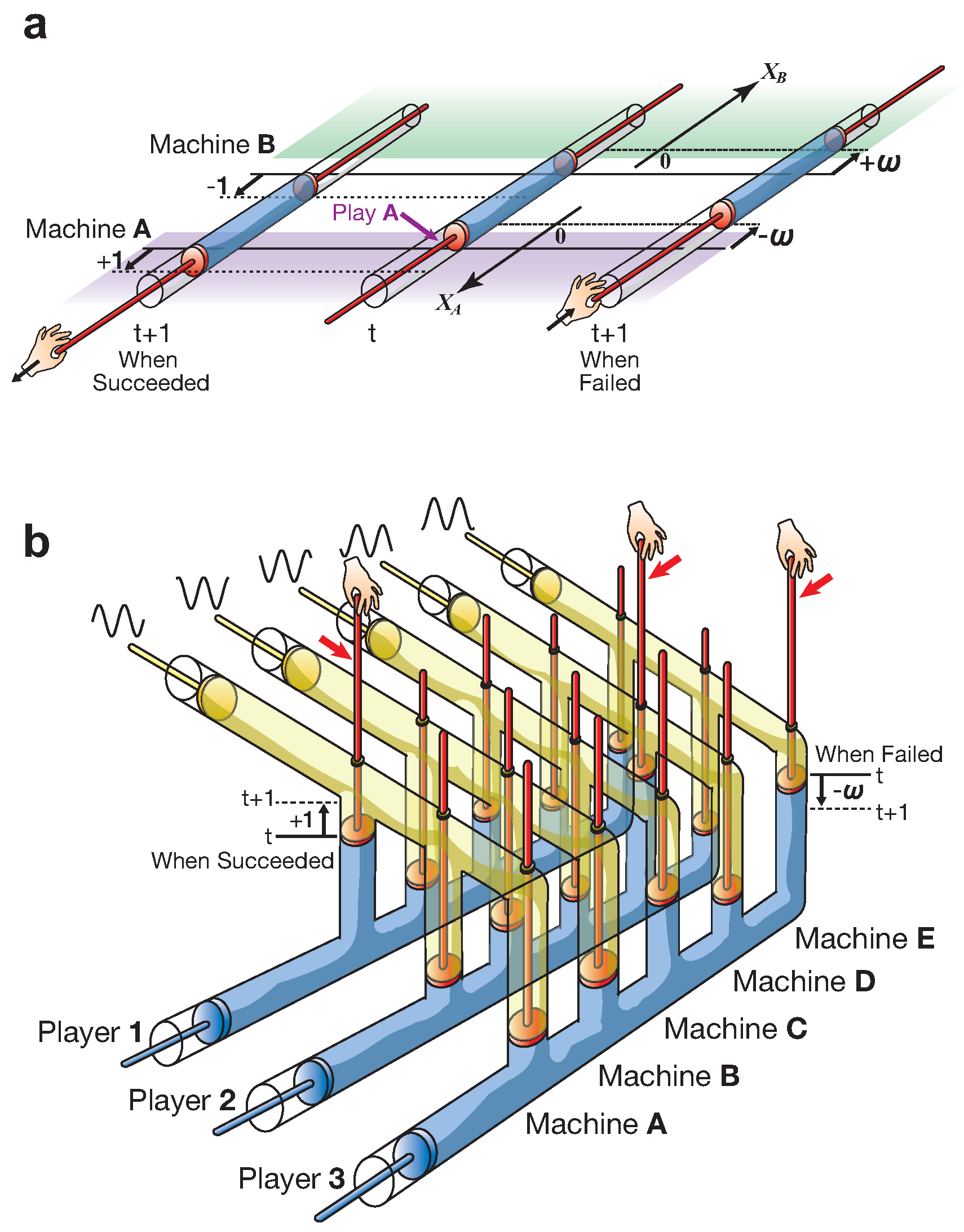
Consider an incompressible fluid in a cylinder, as shown in Figure 2a. Here, X k corresponds to the displacement of terminal k from an initial position, where k { A , B } . If X k is greater than 0, we consider that the liquid selects machine k.
We used the following estimate Q k ( k { A , B } ):
Q k ( t ) = Δ Q k ( t ) + Q k ( t 1 ) .
Here, Δ Q k ( t ) is + 1 or ω according to the result (rewarded or not). Otherwise, it is 0. ω is a weighting parameter (see Method).
The displacement X A ( = X B ) is determined by the following difference equation:
X A ( t + 1 ) = Q A ( t ) Q B ( t ) + δ ( t ) .
Here, δ ( t ) is an arbitrary fluctuation to which the liquid is subject. Consequently, the TOW dynamics evolve according to a particularly simple rule: in addition to the fluctuation, if machine k is played at each time t, + 1 and ω are added to X k ( t ) when rewarded and non-rewarded, respectively (Figure 2a). The authors have shown that these simple dynamics gain more rewards (coins or packet transmissions in cognitive radio) than those obtained by other popular algorithms for solving the BP [11,12,13,14].
Many algorithms for the BP estimate the reward probability of each machine. In most cases, this “estimate” is updated only when the corresponding machine is selected. In contrast, TOW dynamics uses a unique learning method which is equivalent to updating both estimates simultaneously owing to the volume conservation law. TOW dynamics can imitate the system that determines its next moves at time t + 1 in referring to the estimate of each machine, even if it was not selected at time t, as if the two machines were simultaneously selected at time t. This unique feature is one of the sources of the TOW’s high performance [14]. We call this the “TOW principle.” This principle is also applicable to a more general BP (see Method).

1.3. The TOW Bombe

The TOW bombe for three players ( 1 , 2 and 3) and five machines ( A , B , C , D and E) is illustrated in Figure 2b. Two kinds of incompressible fluids (blue and yellow) fill coupled cylinders. The blue (bottom) fluid handles a player’s decisions made, while the yellow (upper) one handles interaction among players. Machine selection of each player at each iteration is determined by the height of a red adjuster (a fluid interface level), and the highest machine is chosen. When the movements of blue and yellow adjusters stabilize to reach equilibrium, the TOW principle in the blue fluid holds for each player. In other words, when one interface rises, the other four interfaces fall, resulting in efficient machine selections. Simultaneously, the action–reaction law holds for the yellow fluid (i.e., if the interface level of player 1 rises, the interface levels of players 2 and 3 fall), contributing collision avoidance, and the TOW bombe can search for an overall optimization solution accurately and quickly. In normal use, however, blue and yellow adjusters must have fixed positions not to move.
The dynamics of the TOW bombe are expressed as follows:
Q ( i , k ) ( t ) = Δ Q ( i , k ) ( t ) + Q ( i , k ) ( t 1 ) 1 M 1 j i Δ Q ( j , k ) ( t ) ,
X ( i , k ) ( t + 1 ) = Q ( i , k ) ( t ) 1 N 1 l k Q ( i , l ) ( t ) + δ ( i , k ) ( t ) .
Here, X ( i , k ) ( t ) is the height of the interface of player i and machine k at iteration step t. If machine k is chosen for player i at time t, Δ Q ( i , k ) ( t ) is + 1 or ω according to the result (rewarded or not). Otherwise, it is 0. δ ( t ) ( i , k ) is an arbitrary fluctuation (see Method).
In addition to the above-mentioned dynamics, some fluctuations or external oscillations are added to X ( i , k ) . These added fluctuations or oscillations are sensitive to the TOW bombe’s performance, because fluctuations represent exploration patterns in the early stage.
Thus, the TOW bombe operates only by adding an operation which raises or lowers the interface level ( + 1 or ω ) according to the result (success or failure of coin gain) for each player (total M times) at each time. After these operations, the interface levels move according to the volume conservation law, calculating the next selection for each player. In each player’s selection, an efficient search is achieved as a result of the TOW principle, which can obtain a solution accurately and quickly for trial-and-error tasks. Moreover, through the interaction among players via yellow fluid, the Nash equilibrium can be avoided, thereby achieving the social maximum [9,10].

2. Results for CBP

To show that the TOW bombe avoids the Nash equilibrium and regularly achieves an overall optimization, we consider a case wherein ( P A , P B , P C , P D , P E ) = ( 0 . 03 , 0 . 05 , 0 . 1 , 0 . 2 , 0 . 9 ) as a typical example. For simplicity, part of the payoff tensor that has 125 (= 5 3 ) elements is described as follows; only matrix elements for which each player does not choose low-ranking A and B are shown (Table 1, Table 2 and Table 3). For each matrix element, the reward probabilities are given in the order of players 1, 2 and 3.
Social maximum (SM) is a state in which the maximum amount of total reward is obtained by all the players. In this problem, the social maximum corresponds to a segregation state in which the players choose the top three distinct machines ( C , D , E ), respectively; there are six segregation states indicated by SM in the Tables. In contrast, the Nash equilibrium (NE) is a state in which all the players choose machine E independent of others’ decisions; machine E gives the reward with the highest probability, when each player behaves selfishly.
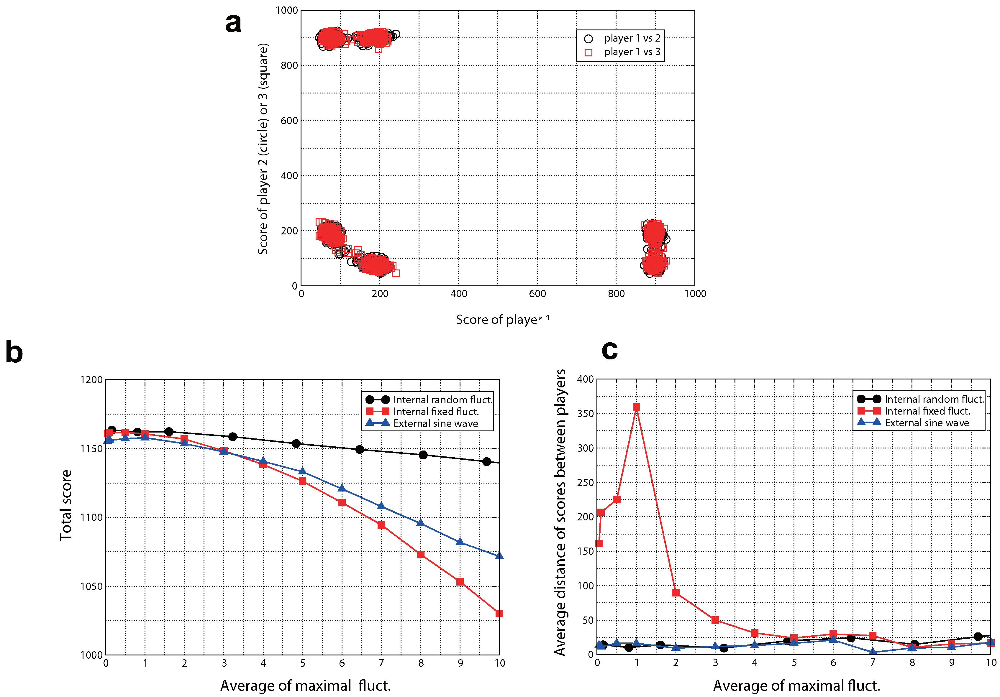
The performance of the TOW bombe was evaluated using a score: the number of rewards (coins) a player obtained in his/her 1000 plays. In cognitive radio communication, the score corresponds to the number of packets that have successfully transmitted [18,19]. Figure 3a shows the TOW bombe scores in the typical example wherein ( P A , P B , P C , P D , P E ) = ( 0 . 03 , 0 . 05 , 0 . 1 , 0 . 2 , 0 . 9 ). Since 1000 samples were used, there are 1000 circles. Each circle indicates the score obtained by player i (horizontal axis) and player j (vertical axis) for one sample. There are six clusters in Figure 3a corresponding to the two-dimensional projections of the six segregation states, implying the overall optimization. The social maximum points are given as follows: (the score of player 1, the score of player 2, the score of player 3) = (100, 200, 900), (100, 900, 200), (200, 100, 900), (200, 900, 100), (900, 100, 200) and (900, 200, 100). The TOW bombe did not reach the Nash equilibrium state (300, 300, 300).
In our simulations, we used “adaptive” weighting parameter ω, meaning that the parameter is estimated by using its own variables (see Method). Owing to this estimation cost, clusters of circles are not located exactly at the social maximum points. If we set weighting parameter ω at 0 . 08 , which are calculated as γ = P B + P C (see Method), those clusters are located exactly on the social maximum points (see Figure 4 in Ref. [22]).
Figure 3b shows TOW bombe performance, sample averages of the total scores of all players up to 1000 plays, for three different types of fluctuation, respectively. The black, red and blue lines denote the cases of internal random fluctuations, internal fixed fluctuations and external oscillations, respectively (see Method). The horizontal axis denotes the sample averages of maximum fluctuation. In the maximal case, the average total score has gained nearly 1200 (=100 + 200 + 900), which is the value of the social maximum, although there are some gaps resulting from estimation costs.
Figure 3c also shows TOW bombe fairness, sample averages of the mean distance between players’ scores, for three different types of fluctuation, respectively. We can confirm lower fairness in the cases of internal fixed fluctuations (red line). Artificially created fluctuations, such as internal fixed fluctuations, often show lower fairness because of the existence of biases (lack of uniformity or randomness) in fluctuations. Although the external oscillations (sine waves) have higher fairness (blue line), controlling the blue and yellow adjusters appropriately is difficult. Moreover, the performances of these two types of fluctuation rapidly decrease as the magnitude of fluctuations increases, as shown in Figure 3b.
We can conclude that only the internal random fluctuations, which are supposed to be generated automatically in the real TOW bombe, exhibit higher performance and fairness. This conclusion is consistent even in cases where we set weighting parameter ω at 0 . 08 . This indicates the construction of a novel analog computing scheme which exploits nature’s power in terms of automatic generation of random fluctuations, simultaneous computations using a conservation law and intrinsic efficiency.

3. Results for the Extended Prisoner’s Dilemma Game

Although the payoff tensor has N M elements, the TOW bombe need not hold N M evaluation values. It is noted that the congestion effects, where each reward probability is divided by the number of players due to the collisions, appeared only in the diagonal elements of the payoff tensor. If we ignore the diagonal elements, N evaluation values are sufficient for each player’s estimation of which machine is the best because the problem becomes independent of the three BPs. Therefore, using the TOW bombe, the CBP is reducible to an O ( N M ) problem when implementing a collision-avoiding mechanism handled by yellow fluid, although, in a strict sense, the computational cost must include the cost for providing random fluctuations generated by the fluids’ physical dynamics. In Figure 3b, we showed the results of only three types of fluctuation. TOW bombe performance with internal M-random fluctuations (see Method) was the same as that of the internal random fluctuations, although computations for generating the former type of fluctuation require a cost that exponentially grows as O ( N M ) . This is because the exponential type of fluctuation is not effective for O ( N M ) problems. Various random seed patterns do not affect enhancing the performance of O ( N M ) problems because of the reducibility of CBP to three independent BPs.
However, this is not the cases if we focus on more complex problems, such as the “Extended Prisoner’s Dilemma Game”; we must prepare more than N M evaluation values because a player’s reward is drastically changed according to the selections of other players in this problem.
Consider a situation wherein three people are arrested by the police and are required to choose from the following five options:
  • A: keep silent;
  • B: confess (implicate him- or herself);
  • C: implicate the next person (circulative as 1,2,3,1,2,3,⋯);
  • D: implicate the third person (circulative as 1,2,3,1,2,3,⋯);
  • E: implicate both of the others.
According to the three person’s choices, the “degree of charges” (from 0 to 3) are to be determined for every person. For example, the degree of charges are ( 1 , 1 , 1 ) for the choice (person 1, person 2, person 3) = (B,B,B), ( 1 , 1 , 0 ) for the choice (A,B,C), ( 2 , 1 , 1 ) for the choice (B,C,D), ( 2 , 2 , 1 ) for the choice (C,D,D), ( 2 , 2 , 2 ) for the choice (D,D,D), ( 3 , 1 , 1 ) for the choice (B,D,D) etc. For each pattern of degree of charges, a set of reward probabilities of each person are determined as follows: in what follows, P, R, R1, R2, S1, S2, S3, T1, T2, and T3 are reward probabilities that specify the problem for players (prisoners). The notation was borrowed from Ref. [23]):
  • the set of reward probabilities for the charges ( 0 , 0 , 0 ) is ( R 2 , R 2 , R 2 );
  • the ( 1 , 1 , 1 ) → ( R 1 , R 1 , R 1 );
  • the ( 2 , 1 , 1 ) or ( 1 , 2 , 1 ) or ( 1 , 1 , 2 ) → (R, R, R): the social maximum;
  • the ( 2 , 2 , 2 ) → (P,P,P): the Nash equilibrium.
Otherwise, each difference between his or her degree and the minimum degree of the pattern determines a reward probability. If his/her degree is the same as the minimum degree, the reward probability is “T,” otherwise “S.” Moreover, the difference between his or her degree and the minimum degree of the pattern is added to it. For example, the ( 1 , 1 , 0 ) → ( S 1 , S 1 , T 1 ), the ( 2 , 2 , 1 ) → ( S 1 , S 1 , T 1 ), the ( 3 , 1 , 1 ) → ( S 2 , T 2 , T 2 ). Here, we set T 3 = 0 . 79 , T 2 = 0 . 76 , T 1 = 0 . 73 , R = 0 . 70 , R 1 = 0 . 60 , R 2 = 0 . 55 , P = 0 . 50 , S 1 = 0 . 40 , S 2 = 0 . 30 and S 3 = 0 . 20 . Therefore, the social maximum is (R,R,R). Here, charges (2, 1, 1), (1, 2, 1), and (1, 1, 2) are special states from which the police cannot extract any information because it is assumed that the police know in advance that there are one main suspect and two accomplices in the problem setting. We treat as exceptional states those where the same R is assigned to all the prisoners, although their charges are different. The complete list of reward probabilities is shown in Table 4.
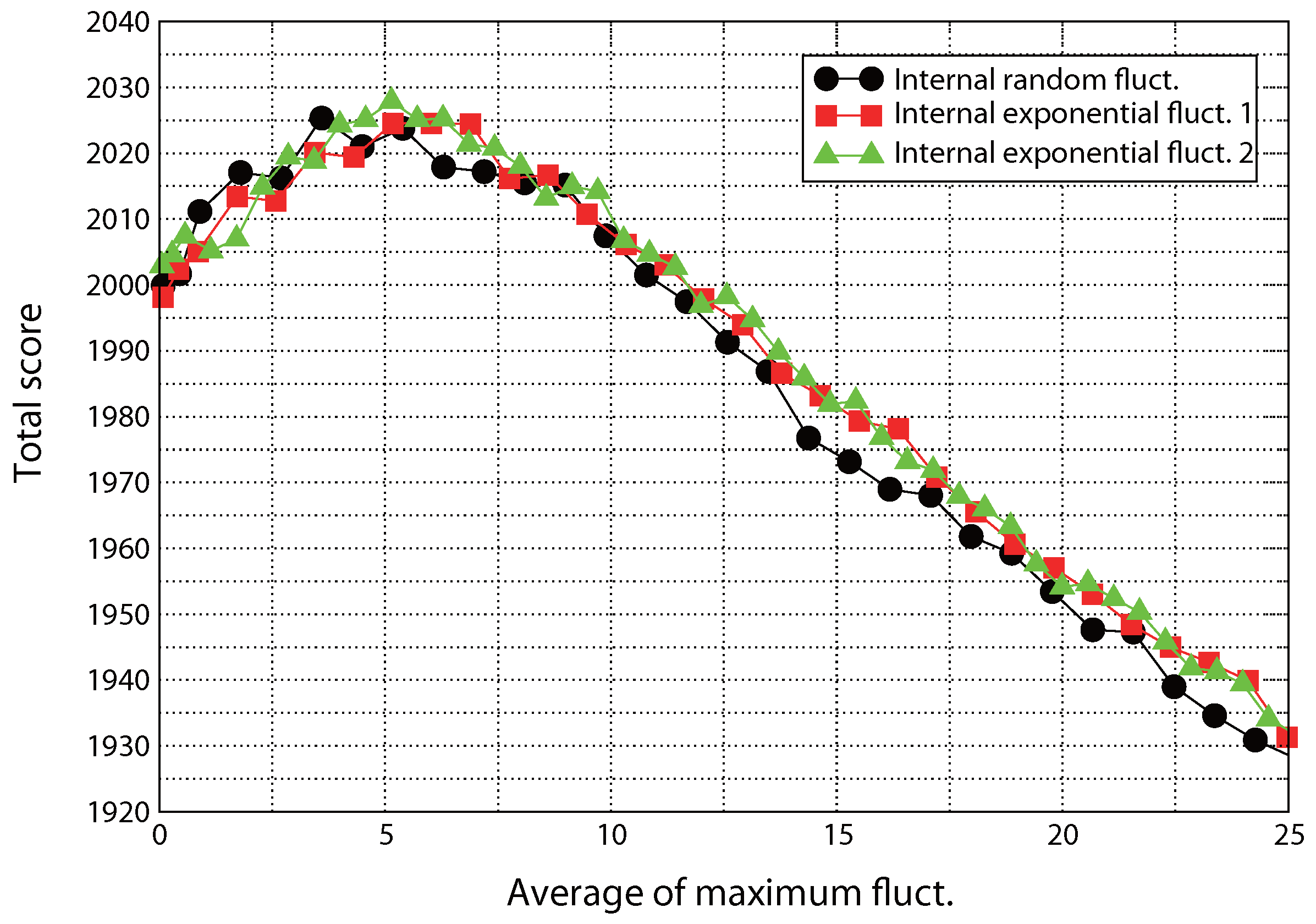
If we allow ourselves to consider approximate solutions, some of the problems in the complex classes would be solved efficiently using the TOW bombe, as the complexity of these problems has approximate reducibility to O ( N M ) . In these cases, the exponential type of fluctuation can enhance the performance very slightly (see Figure 4). This fact may suggest that we find the first toehold to harnessing nature’s power which is the feasibility of massive computations. However, it is difficult to solve this type of complex problem using the TOW bombe in general. To solve more complex problems and find the toehold, we must also extend the TOW bombe.

4. Conclusions

The TOW bombe enables us to solve the assignment problem for M players and N machines by repeating M up-and-down operations of fluid interface levels in cylinders at each iteration; it does not require calculation for as many evaluation values as are required when using a conventional digital computer because it entrusts the huge amount of computation to the physical processes of fluids. This suggests that there are advantages to analog computation even in today’s digital age. Moreover, higher performance is produced by using internal random fluctuations, which are supposed to be generated physically in the materially-implemented TOW bombe, rather than by using artificially-generated fluctuations.

5. Discussion

Introducing the TOW bombe, we extracted a method to harness the computational power of nature from fluid dynamics; the TOW bombe exploits (1) the physical generation of random fluctuations; (2) simultaneous (concurrent) computations via the conservation law; and (3) its intrinsic efficiency [14]. Another significant aspect of fluids from which we tried to exploit computational power is their capacity to produce “genuine randomness”, which is generated through the fluctuating movements of the massive number of molecules of which they are comprised. We represented the fluid-derived fluctuations as “M-random fluctuations” by making exponentially-many combinatorial efforts. However, we were unable to satisfactorily exploit the power of M-random fluctuations. This is because, as long as we use the current configuration of the TOW bombe, we cannot accommodate a class of problems whose complexity cannot be reduced to O ( N M ) . Therefore, we need to extend the configuration of the TOW bombe so that it can be applied to solving more complex classes of problems, such as the “Extended Prisoner’s Dilemma Game” and others with O ( N M ) complexity.
Unfortunately, it is difficult to solve the “Extended Prisoner’s Dilemma Game” type of complex problem using the TOW bombe in general. We have some ideas regarding TOW bombe extension using some fluid compressibility, local inflow and outflow, a reservoir for blue or yellow fluid, a time order of fluctuations and quantum effects such as non-locality and entanglement. If we assume the relaxation processes of fluids, we can extend our model so that it can exploit more flexible dynamical effects from the movements of fluids, such as those originating from velocity-dependent reaction, delay, dissipation and synchronization. If we successfully extend the TOW bombe, all possible multiplayer decision-making problems in our framework could be solved. We will also investigate whether our approach confronts some of the fundamental difficulties considered in “Arrow’s impossibility theorem [24]”. The TOW bombe can also be implemented on the basis of quantum physics. In fact, the authors have exploited optical energy transfer dynamics between quantum dots and single photons to design decision-making devices [25,26,27,28]. Our method might be applicable to a class of problems derived from CBP and broader varieties of game payoff tensors, implying that wider applications can be expected. We will report these observations and results elsewhere in the future.

Methods

The Weighting Parameter ω

TOW dynamics involves the parameter ω which is sensitive to its performance. From analytical calculations, it is known that the following ω 0 is sub-optimal in the BP (see [14]):
ω 0 = γ 2 γ ,
γ = P A + P B ,
where it is assumed that P A is the largest reward probability and P B is the second largest.
In the CBP cases (M-player and N-machine), the following ω 0 is sub-optimal:
ω 0 = γ 2 γ ,
γ = P ( M ) + P ( M + 1 ) ,
where P ( M ) is the top Mth reward probability.
Players must estimate ω 0 using its variables because information regarding reward probabilities is not given to players. We call this an “adaptive” weighting parameter. There are many estimate methods, such as Bayesian inference, but we simply use “direct substitution” herein. Direct substitution uses R j ( t ) / N j ( t ) for P j , where R j ( t ) is the number of reward gains from machine j through time t and N j ( t ) is the number of plays of machine j through time t.

TOW Dynamics for General BP

In this paper, we use TOW dynamics only for the Bernoulli type of BP in which the reward r is 1 or 0. Another type of TOW dynamics can also be constructed for general BP in which the reward r is a real value from an interval [ 0 , R ] . Here, R is arbitrary positive value, and the reward r is selected according to given probability distribution whose mean and variance are μ and σ 2 , respectively.
In this case, the following estimate Q k ( k { A , B } ) is used instead of Equation (1):
Q k ( t ) = Σ j = 1 t r k ( j ) γ N k ( t ) .
Here, N k is the number of playing machine k until time t and r k ( j ) is the reward in k at time j, where γ is the following parameter:
γ = μ A + μ B 2 .
If machine k is played at each time t, the reward r k ( t ) and γ are added to X k ( t 1 ) .

Generating Methods of Fluctuations

Internal Fixed Fluctuations

First, we define fixed moves O k ( k = 0 , , 4 ), as follows:
{ O 0 , O 1 , O 2 , O 3 , O 4 } = { 0 , A , 0 , A , 0 . }
where A is an amplitude parameter. Note that k = 0 4 O k = 0.
To use the above move O k recursively, we introduce a new variable n u m ( n u m = 0 , , 4 ), as follows:
n u m = { t + ( k 2 ) } m o d 5 .
Here, t is a time. For each machine k ( k = 1 , , 5 ), we use the following set of fluctuations, respectively:
o s c ( 1 , k ) ( t ) = O 0 ,
o s c ( 2 , k ) ( t ) = O 3 ,
o s c ( 3 , k ) ( t ) = O 1 ,
if n u m = 0;
o s c ( 1 , k ) ( t ) = O 1 ,
o s c ( 2 , k ) ( t ) = O 4 ,
o s c ( 3 , k ) ( t ) = O 3 ,
if n u m = 1;
o s c ( 1 , k ) ( t ) = O 2 ,
o s c ( 2 , k ) ( t ) = O 0 ,
o s c ( 3 , k ) ( t ) = O 4 ,
if n u m = 2;
o s c ( 1 , k ) ( t ) = O 3 ,
o s c ( 2 , k ) ( t ) = O 1 ,
o s c ( 3 , k ) ( t ) = O 2 ,
if n u m = 3;
o s c ( 1 , k ) ( t ) = O 4 ,
o s c ( 2 , k ) ( t ) = O 2 ,
o s c ( 3 , k ) ( t ) = O 0 ,
if n u m = 4.
It always holds that i = 1 3 o s c ( i , k ) ( t ) = 0 and k = 1 5 o s c ( i , k ) ( t ) = 0. These conditions mean that added fluctuations to X ( i , k ) can be cancelled in total. In other words, the total volume of blue or yellow fluid does not change. As a result, we create artificial “internal” fluctuations.

Internal Random Fluctuations

First, a matrix sheet of random fluctuations ( S h e e t ( i , k ) ) is prepared. Here, i = 1 , , 3 and k = 1 , , 5 .
  • r is a random value from [ 0 , 1 ] . We call this “seed”.
  • There are N M ( = 15 ) possibilities for a seed position. Choose the seed position ( i 0 , k 0 ) randomly from i 0 = 1 , , 3 and k 0 = 1 , , 5 and place the seed r at the point,
    S h e e t ( i 0 , k 0 ) = r .
  • All elements of the k 0 th column other than ( i o , k 0 ) are substituted with 0 . 5 r .
  • All elements of the i 0 -th row other than ( i o , k 0 ) are substituted with 0 . 25 r .
  • All remaining elements are substituted with r / 8 . 0 .
  • The matrix sheet is summed up in a summation matrix S u m ( i , k ) .
  • Repeat from two to six for D times. Here, D is a parameter.
We used the following set of fluctuations:
o s c ( i , k ) ( t ) = A / D S u m ( i , k ) ,
where A is an amplitude parameter.
It always holds that i = 1 3 o s c ( i , k ) ( t ) = 0 and k = 1 5 o s c ( i , k ) ( t ) = 0, as well as the internal fixed fluctuations. The total volume of blue or yellow fluid does not change. As a result, we create “internal” random fluctuations naturally. At every time step, this procedure costs O ( N · M ) computations with a digital computer.

Internal M-Random Fluctuations (Exponential)

First, a matrix sheet of random fluctuations ( S h e e t ( i , k ) ) is prepared. Here, i = 1 , , 3 and k = 1 , , 5 .
  • For each player i, independent random value r i is generated from [ 0 , 1 ] . We call these “seeds”.
  • There are N M ( = 125 ) possibilities for a seed position pattern. For each player i, choose the seed position (i, k 0 ( i ) ) randomly from k 0 ( i ) = 1 , , 5 and place the seed r i at the point
    S h e e t ( i , k 0 ( i ) ) = r i .
    However, we choose k 0 ( i ) s to be distinct. Therefore, there are really N ( N 1 ) ( N 2 ) (=60) possibilities.
  • For each i, all elements of the k 0 ( i ) -th column other than (i, k 0 ( i ) ) are substituted with 0 . 5 r i .
  • All remaining elements of the 1th row are substituted with 0 . 50 ( r 1 0 . 50 r 2 0 . 50 r 3 ) .
  • All remaining elements of the 2th row are substituted with 0 . 50 ( r 2 0 . 50 r 1 0 . 50 r 3 ) .
  • All remaining elements of the 3th row are substituted with 0 . 50 ( r 3 0 . 50 r 1 0 . 50 r 2 ) .
  • The matrix sheet is summed up in a summation matrix S u m ( i , k ) .
  • Repeat from two to seven for D times. Here, D is a parameter.
We used the following set of fluctuations:
o s c ( i , k ) = A / D S u m ( i , k ) ,
where A is an amplitude parameter.
It always holds that i = 1 3 o s c ( i , k ) ( t ) = 0 and k = 1 5 o s c ( i , k ) ( t ) = 0 as well as the internal fixed or random fluctuations. The total volume of blue or yellow fluid does not change. As a result, we create “internal” M-random fluctuations naturally. At every time step, this procedure costs exponential computations of O ( N M ) with a digital computer.

External Oscillations

Herein, we used completely synchronised oscillations o s c ( i , k ) ( t ) added to every player’s X ( i , k ) ,
o s c ( i , k ) ( t ) = A s i n ( 2 π t / 5 + 2 π ( k 1 ) / 5 ) ,
where i = 1 , ⋯, 3 and k = 1 , ⋯, 5. A is an amplitude parameter. These oscillations are externally provided by appropriately controlling the blue and yellow adjusters.

Acknowledgments

This work was supported in part by MEXT/JSPS KAKENHI 15K13387 (Grand-in-Aid for Challenging Exploratory Research). We are grateful to Hirokazu Hori at the University of Yamanashi for useful arguments about the theory of the TOW bombe and its quantum extension.

Author Contributions

Song-Ju Kim and Masashi Aono designed the research. Song-Ju Kim designed and simulated the TOW Bombe. Song-Ju Kim, Masashi Aono and Makoto Naruse analysed the data. Song-Ju Kim and Masashi Aono wrote the manuscript. All authors reviewed the manuscript.

Conflicts of Interest

The authors declare no conflict of interest.

References

  1. Mesquita BBDe. The Predictioneer’s Game; Random House Inc.: New York, NY, USA, 2009. [Google Scholar]
  2. Narendra, K.S.; Member, S.; Thathachar, M.A.L. Learning automata—A survey. IEEE Trans. Syst. Man Cybern. 1974, SMC-4, 323–334. [Google Scholar] [CrossRef]
  3. Fudenberg, D.; Levine, D.K. The Theory of Learning in Games; The MIT Press: Cambridge, MA, USA, 1998. [Google Scholar]
  4. Marden, J.R.; Young, H.P.; Arslan, G.; Shamma, J. Payoff based dynamics for multiplayer weakly acyclic games. SIAM J. Control Optim. 2009, 48, 373–396. [Google Scholar] [CrossRef]
  5. Turing, A.M. On computable numbers, with an application to the Entscheidungsproblem. Proc. Lond. Math. Soc. 1936, 42, 230–265. [Google Scholar]
  6. Turing, A.M. Computability and λ-definability. J. Symb. Log. 1937, 2, 153–163. [Google Scholar] [CrossRef]
  7. Moore, C. A complex legacy. Nat. Phys. 2011, 7, 828–830. [Google Scholar] [CrossRef]
  8. Feynman, R.P. Feynman Lectures on Computation; Perseus Books: New York, NY, USA, 1996. [Google Scholar]
  9. Roughgarden, T. Selfish Routing and the Price of Anarchy; The MIT Press: Cambridge, MA, USA, 2005. [Google Scholar]
  10. Nisan, N.; Roughgarden, T.; Tardos, E.; Vazirani, V.V. Algorithmic Game Theory; Cambridge University Press: New York, NY, USA, 2007. [Google Scholar]
  11. Kim, S.-J.; Aono, M.; Hara, M. Tug-of-war model for multi-armed bandit problem. In Unconventional Computation; LNCS 6079; Calude, C.S., Hagiya, M., Morita, K., Rozenberg, G., Timmis, J., Eds.; Springer: Berlin/Heidelberg, Germany, 2010; pp. 69–80. [Google Scholar]
  12. Kim, S.-J.; Aono, M.; Hara, M. Tug-of-war model for two-bandit problem: Nonlocally correlated parallel exploration via resource conservation. BioSystems 2010, 101, 29–36. [Google Scholar] [CrossRef] [PubMed]
  13. Kim, S.-J.; Aono, M. Amoeba-inspired algorithm for cognitive medium access. NOLTA 2014, 5, 198–209. [Google Scholar] [CrossRef]
  14. Kim, S.-J.; Aono, M.; Nameda, E. Efficient decision-making by volume-conserving physical object. New J. Phys. 2015, 17, 083023. [Google Scholar] [CrossRef]
  15. Auer, P.; Cesa-Bianchi, N.; Fischer, P. Finite-time analysis of the multiarmed bandit problem. Mach. Learn. 2002, 47, 235–256. [Google Scholar] [CrossRef]
  16. Kocsis, L.; Szepesvári, C. Bandit based monte-carlo planning. In Proceedings of the 17th European Conference on Machine Learning, Berlin, Germany, 18–22 September 2006; LNAI 4212. Springer: Berlin/Heidelberg, Germany, 2006; pp. 282–293. [Google Scholar]
  17. Gelly, S.; Wang, Y.; Munos, R.; Teytaud, O. Modification of UCT with Patterns in Monte-Carlo Go. (Research Report) RR-6062. 2006, pp. 1–19. Available online: https://hal.inria.fr/inria-00117266/document (accessed on 6 December 2016).
  18. Lai, L.; Jiang, H.; Poor, H.V. Medium access in cognitive radio networks: A competitive multi-armed bandit framework. In Proceedings of the IEEE 42nd Asilomar Conference on Signals, System and Computers, Pacific Grove, CA, USA, 26–29 October 2008; pp. 98–102.
  19. Lai, L.; Gamal, H.E.; Jiang, H.; Poor, H.V. Cognitive medium access: Exploration, exploitation, and competition. IEEE Trans. Mob. Comput. 2011, 10, 239–253. [Google Scholar]
  20. Agarwal, D.; Chen, B.-C.; Elango, P. Explore/exploit schemes for web content optimization. In Proceedings of the Ninth IEEE International Conference on Data Mining, Miami, FL, USA, 6–9 December 2009.
  21. Davies, D. The Bombe—A remarkable logic machine. Cryptologia 1999, 23, 108–138. [Google Scholar] [CrossRef]
  22. Kim, S.-J.; Aono, M. Decision maker using coupled incompressible-fluid cylinders. Adv. Sci. Technol. Environmentol. 2015, B11, 41–45. [Google Scholar]
  23. Helbing, D.; Yu, W. The outbreak of cooperation among success-driven individuals under noisy conditions. Proc. Natl. Acad. Sci. USA 2009, 106, 3680–3685. [Google Scholar] [CrossRef] [PubMed]
  24. Arrow, K.J. A difficulty in the concept of social welfare. J. Political Econ. 1950, 58, 328–346. [Google Scholar] [CrossRef]
  25. Kim, S.-J.; Naruse, M.; Aono, M.; Ohtsu, M.; Hara, M. Decision maker based on nanoscale photo-excitation transfer. Sci. Rep. 2013, 3, 2370. [Google Scholar] [CrossRef] [PubMed]
  26. Naruse, M.; Nomura, W.; Aono, M.; Ohtsu, M.; Sonnefraud, Y.; Drezet, A.; Huant, S.; Kim, S.-J. Decision making based on optical excitation transfer via near-field interactions between quantum dots. J. Appl. Phys. 2014, 116, 154303. [Google Scholar] [CrossRef] [Green Version]
  27. Naruse, M.; Berthel, M.; Drezet, A.; Huant, S.; Aono, M.; Hori, H.; Kim, S.-J. Single photon decision maker. Sci. Rep. 2015, 5, 13253. [Google Scholar] [CrossRef] [PubMed]
  28. Kim, S.-J.; Tsuruoka, T.; Hasegawa, T.; Aono, M.; Terabe, K.; Aono, M. Decision maker based on atomic switches. AIMS Mater. Sci. 2016, 3, 245–259. [Google Scholar] [CrossRef]
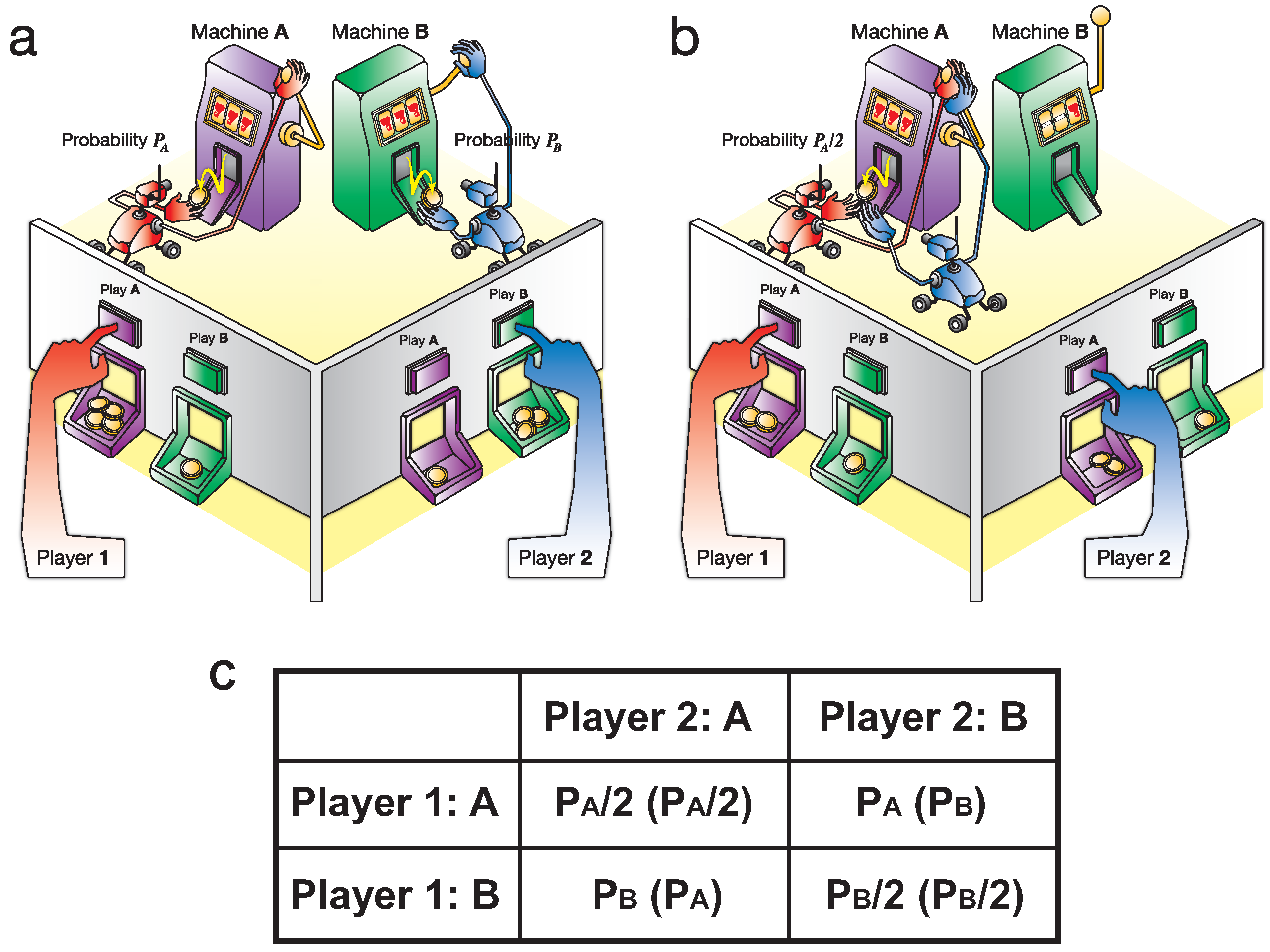
Figure 1. Competitive bandit problem (CBP). (a) segregation state; (b) collision state; and (c) payoff matrix for player 1 (player 2).
Philosophies 01 00245 g001
Figure 2. (a) TOW dynamics; and (b) the TOW bombe for three players and five channels.
Philosophies 01 00245 g002
Figure 3. (a) scores of the TOW bombe in the typical example where ( P A , P B , P C , P D , P E ) = ( 0 . 03 , 0 . 05 , 0 . 1 , 0 . 2 , 0 . 9 ); (b) sample averages of total scores of the TOW bombe in the case where ( P A , P B , P C , P D , P E ) = ( 0 . 03 , 0 . 05 , 0 . 1 , 0 . 2 , 0 . 9 ); and (c) sample averages of mean distance between player’s scores in the case where ( P A , P B , P C , P D , P E ) = ( 0 . 03 , 0 . 05 , 0 . 1 , 0 . 2 , 0 . 9 ).
Philosophies 01 00245 g003
Figure 4. Sample averages of total scores of the TOW bombe in the Extended Prisoner’s Dilemma Game.
Philosophies 01 00245 g004
Table 1. Payoff matrix of the case where ( P C , P D , P E ) = ( 0 . 1 , 0 . 2 , 0 . 9 ), player 3 chooses C.
Player 2: CPlayer 2: DPlayer 2: E
player 1: C 1 / 30 , 1 / 30 , 1 / 30 0 . 05 , 0 . 2 , 0 . 05 0 . 05 , 0 . 9 , 0 . 05
player 1: D 0 . 2 , 0 . 05 , 0 . 05 0 . 1 , 0 . 1 , 0 . 1 0 . 2 , 0 . 9 , 0 . 1 SM
player 1: E 0 . 9 , 0 . 05 , 0 . 05 0 . 9 , 0 . 2 , 0 . 1 SM 0 . 45 , 0 . 45 , 0 . 1
Table 2. Payoff matrix of the case where ( P C , P D , P E ) = ( 0 . 1 , 0 . 2 , 0 . 9 ), player 3 chooses D.
Player 2: CPlayer 2: DPlayer 2: E
player 1: C 0 . 05 , 0 . 05 , 0 . 2 0 . 1 , 0 . 1 , 0 . 1 0 . 1 , 0 . 9 , 0 . 2 SM
player 1: D 0 . 1 , 0 . 1 , 0 . 1 2 / 30 , 2 / 30 , 2 / 30 0 . 1 , 0 . 9 , 0 . 1
player 1: E 0 . 9 , 0 . 1 , 0 . 2 SM 0 . 9 , 0 . 1 , 0 . 1 0 . 45 , 0 . 45 , 0 . 2
Table 3. Payoff matrix of the case where ( P C , P D , P E ) = ( 0 . 1 , 0 . 2 , 0 . 9 ), player 3 chooses E.
Player 2: CPlayer 2: DPlayer 2: E
player 1: C 0 . 05 , 0 . 05 , 0 . 9 0 . 1 , 0 . 2 , 0 . 9 SM 0 . 1 , 0 . 45 , 0 . 45
player 1: D 0 . 2 , 0 . 1 , 0 . 9 SM 0 . 1 , 0 . 1 , 0 . 9 0 . 2 , 0 . 45 , 0 . 45
player 1: E 0 . 45 , 0 . 1 , 0 . 45 0 . 45 , 0 . 2 , 0 . 45 0 . 3 , 0 . 3 , 0 . 3 NE
Table 4. Reward probabilities in the Extended Prisoner’s Dilemma Game.
Selection PatternDegree of ChargesProbability
( A, A, A )( 0, 0, 0 )0.55 0.55 0.55
( A, A, B )( 0, 0, 1 )0.73 0.73 0.40
( A, A, C )( 1, 0, 0 )0.40 0.73 0.73
( A, A, D )( 0, 1, 0 )0.73 0.40 0.73
( A, A, E )( 1, 1, 0 )0.40 0.40 0.73
( A, B, A )( 0, 1, 0 )0.73 0.40 0.73
( A, B, B )( 0, 1, 1 )0.73 0.40 0.40
( A, B, C )( 1, 1, 0 )0.40 0.40 0.73
( A, B, D )( 0, 2, 0 )0.76 0.30 0.76
( A, B, E )( 1, 2, 0 )0.73 0.30 0.76
( A, C, A )( 0, 0, 1 )0.73 0.73 0.40
( A, C, B )( 0, 0, 2 )0.76 0.76 0.30
( A, C, C )( 1, 0, 1 )0.40 0.73 0.40
( A, C, D )( 0, 1, 1 )0.73 0.40 0.40
( A, C, E )( 1, 1, 1 )0.60 0.60 0.60
( A, D, A )( 1, 0, 0 )0.40 0.73 0.73
( A, D, B )( 1, 0, 1 )0.40 0.73 0.40
( A, D, C )( 2, 0, 0 )0.30 0.76 0.76
( A, D, D )( 1, 1, 0 )0.40 0.40 0.73
( A, D, E )( 2, 1, 0 )0.30 0.73 0.76
( A, E, A )( 1, 0, 1 )0.40 0.73 0.40
( A, E, B )( 1, 0, 2 )0.73 0.76 0.30
( A, E, C )( 2, 0, 1 )0.30 0.76 0.73
( A, E, D )( 1, 1, 1 )0.60 0.60 0.60
( A, E, E )( 2, 1, 1 )0.70 0.70 0.70
( B, A, A )( 1, 0, 0 )0.40 0.73 0.73
( B, A, B )( 1, 0, 1 )0.40 0.73 0.40
( B, A, C )( 2, 0, 0 )0.30 0.76 0.76
( B, A, D )( 1, 1, 0 )0.40 0.40 0.73
( B, A, E )( 2, 1, 0 )0.30 0.73 0.76
( B, B, A )( 1, 1, 0 )0.40 0.40 0.73
( B, B, B )( 1, 1, 1 )0.60 0.60 0.60
( B, B, C )( 2, 1, 0 )0.30 0.73 0.76
( B, B, D )( 1, 2, 0 )0.73 0.30 0.76
( B, B, E )( 2, 2, 0 )0.30 0.30 0.76
( B, C, A )( 1, 0, 1 )0.40 0.73 0.40
( B, C, B )( 1, 0, 2 )0.73 0.76 0.30
( B, C, C )( 2, 0, 1 )0.30 0.76 0.73
( B, C, D )( 1, 1, 1 )0.60 0.60 0.60
( B, C, E )( 2, 1, 1 )0.70 0.70 0.70
( B, D, A )( 2, 0, 0 )0.30 0.76 0.76
( B, D, B )( 2, 0, 1 )0.30 0.76 0.73
( B, D, C )( 3, 0, 0 )0.20 0.79 0.79
( B, D, D )( 2, 1, 0 )0.30 0.73 0.76
( B, D, E )( 3, 1, 0 )0.20 0.76 0.79
( B, E, A )( 2, 0, 1 )0.30 0.76 0.73
( B, E, B )( 2, 0, 2 )0.30 0.76 0.30
( B, E, C )( 3, 0, 1 )0.20 0.79 0.76
( B, E, D )( 2, 1, 1 )0.70 0.70 0.70
( B, E, E )( 3, 1, 1 )0.30 0.76 0.76
( C, A, A )( 0, 1, 0 )0.73 0.40 0.73
( C, A, B )( 0, 1, 1 )0.73 0.40 0.40
( C, A, C )( 1, 1, 0 )0.40 0.40 0.73
( C, A, D )( 0, 2, 0 )0.76 0.30 0.76
( C, A, E )( 1, 2, 0 )0.73 0.30 0.76
( C, B, A )( 0, 2, 0 )0.76 0.30 0.76
( C, B, B )( 0, 2, 1 )0.76 0.30 0.73
( C, B, C )( 1, 2, 0 )0.73 0.30 0.76
( C, B, D )( 0, 3, 0 )0.79 0.20 0.79
( C, B, E )( 1, 3, 0 )0.76 0.20 0.79
( C, C, A )( 0, 1, 1 )0.73 0.40 0.40
( C, C, B )( 0, 1, 2 )0.76 0.73 0.30
( C, C, C )( 1, 1, 1 )0.60 0.60 0.60
( C, C, D )( 0, 2, 1 )0.76 0.30 0.73
( C, C, E )( 1, 2, 1 )0.70 0.70 0.70
( C, D, A )( 1, 1, 0 )0.40 0.40 0.73
( C, D, B )( 1, 1, 1 )0.60 0.60 0.60
( C, D, C )( 2, 1, 0 )0.30 0.73 0.76
( C, D, D )( 1, 2, 0 )0.73 0.30 0.76
( C, D, E )( 2, 2, 0 )0.30 0.30 0.76
( C, E, A )( 1, 1, 1 )0.60 0.60 0.60
( C, E, B )( 1, 1, 2 )0.70 0.70 0.70
( C, E, C )( 2, 1, 1 )0.70 0.70 0.70
( C, E, D )( 1, 2, 1 )0.70 0.70 0.70
( C, E, E )( 2, 2, 1 )0.40 0.40 0.73
( D, A, A )( 0, 0, 1 )0.73 0.73 0.40
( D, A, B )( 0, 0, 2 )0.76 0.76 0.30
( D, A, C )( 1, 0, 1 )0.40 0.73 0.40
( D, A, D )( 0, 1, 1 )0.73 0.40 0.40
( D, A, E )( 1, 1, 1 )0.60 0.60 0.60
( D, B, A )( 0, 1, 1 )0.73 0.40 0.40
( D, B, B )( 0, 1, 2 )0.76 0.73 0.30
( D, B, C )( 1, 1, 1 )0.60 0.60 0.60
( D, B, D )( 0, 2, 1 )0.76 0.30 0.73
( D, B, E )( 1, 2, 1 )0.70 0.70 0.70
( D, C, A )( 0, 0, 2 )0.76 0.76 0.30
( D, C, B )( 0, 0, 3 )0.79 0.79 0.20
( D, C, C )( 1, 0, 2 )0.73 0.76 0.30
( D, C, D )( 0, 1, 2 )0.76 0.73 0.30
( D, C, E )( 1, 1, 2 )0.70 0.70 0.70
( D, D, A )( 1, 0, 1 )0.40 0.73 0.40
( D, D, B )( 1, 0, 2 )0.73 0.76 0.30
( D, D, C )( 2, 0, 1 )0.30 0.76 0.73
( D, D, D )( 1, 1, 1 )0.60 0.60 0.60
( D, D, E )( 2, 1, 1 )0.70 0.70 0.70
( D, E, A )( 1, 0, 2 )0.73 0.76 0.30
( D, E, B )( 1, 0, 3 )0.76 0.79 0.20
( D, E, C )( 2, 0, 2 )0.30 0.76 0.30
( D, E, D )( 1, 1, 2 )0.70 0.70 0.70
( D, E, E )( 2, 1, 2 )0.40 0.73 0.40
( E, A, A )( 0, 1, 1 )0.73 0.40 0.40
( E, A, B )( 0, 1, 2 )0.76 0.73 0.30
( E, A, C )( 1, 1, 1 )0.60 0.60 0.60
( E, A, D )( 0, 2, 1 )0.76 0.30 0.73
( E, A, E )( 1, 2, 1 )0.70 0.70 0.70
( E, B, A )( 0, 2, 1 )0.76 0.30 0.73
( E, B, B )( 0, 2, 2 )0.76 0.30 0.30
( E, B, C )( 1, 2, 1 )0.70 0.70 0.70
( E, B, D )( 0, 3, 1 )0.79 0.20 0.76
( E, B, E )( 1, 3, 1 )0.76 0.30 0.76
( E, C, A )( 0, 1, 2 )0.76 0.73 0.30
( E, C, B )( 0, 1, 3 )0.79 0.76 0.20
( E, C, C )( 1, 1, 2 )0.70 0.70 0.70
( E, C, D )( 0, 2, 2 )0.76 0.30 0.30
( E, C, E )( 1, 2, 2 )0.73 0.40 0.40
( E, D, A )( 1, 1, 1 )0.60 0.60 0.60
( E, D, B )( 1, 1, 2 )0.70 0.70 0.70
( E, D, C )( 2, 1, 1 )0.70 0.70 0.70
( E, D, D )( 1, 2, 1 )0.70 0.70 0.70
( E, D, E )( 2, 2, 1 )0.40 0.40 0.73
( E, E, A )( 1, 1, 2 )0.70 0.70 0.70
( E, E, B )( 1, 1, 3 )0.76 0.76 0.30
( E, E, C )( 2, 1, 2 )0.40 0.73 0.40
( E, E, D )( 1, 2, 2 )0.73 0.40 0.40
( E, E, E )( 2, 2, 2 )0.50 0.50 0.50