
Hiding Full-Color Images into Audio with Visual Enhancement via Residual Networks

Department of Electronic Engineering, National I-Lan University, No. 1, Sec. 1, Shen-Lung Road, I-Lan 26047, Taiwan
*
Author to whom correspondence should be addressed.
Cryptography 2023, 7(4), 47; https://doi.org/10.3390/cryptography7040047
Submission received: 30 August 2023
/
Revised: 18 September 2023
/
Accepted: 25 September 2023
/
Published: 29 September 2023
Abstract
:Watermarking is a viable approach for safeguarding the proprietary rights of digital media. This study introduces an innovative fast Fourier transform (FFT)-based phase modulation (PM) scheme that facilitates efficient and effective blind audio watermarking at a remarkable rate of 508.85 numeric values per second while still retaining the original quality. Such a payload capacity makes it possible to embed a full-color image of 64 × 64 pixels within an audio signal of just 24.15 s. To bolster the security of watermark images, we have also implemented the Arnold transform in conjunction with chaotic encryption. Our comprehensive analysis and evaluation confirm that the proposed FFT–PM scheme exhibits exceptional imperceptibility, rendering the hidden watermark virtually undetectable. Additionally, the FFT–PM scheme shows impressive robustness against common signal-processing attacks. To further enhance the visual rendition of the recovered color watermarks, we propose using residual neural networks to perform image denoising and super-resolution reconstruction after retrieving the watermarks. The utilization of the residual networks contributes to noticeable improvements in perceptual quality, resulting in higher levels of zero-normalized cross-correlation in cases where the watermarks are severely damaged.
1. Introduction
In today’s digital era, a vast array of multimedia data, spanning text, images, audio, and videos, are stored in digital formats for easy distribution and retrieval across the Internet. Correspondingly, digital watermarking emerges as a pivotal technology to safeguard the proprietary rights associated with multimedia content [1]. When content faces the threat of misappropriation or plagiarism, the presence of proprietary information (called the watermark) embedded within the host media can promptly unveil illicit attempts.
In this study, our primary focus centers on the pragmatic aspects of audio watermarking. Although researchers have explored the watermarking technology for decades, there is still much room before its widespread adoption by the general public. One conjecture for this phenomenon could be the absence of captivating applications and appealing operational modes. For audio watermarking, the considerations typically hinge on three critical criteria: payload capacity, imperceptibility, and robustness. Capacity pertains to the volume of information embedded in the host audio. Imperceptibility gauges the extent to which the audio’s fidelity remains intact after watermarking, while robustness signifies the resilience against malicious attacks or unintentional alterations during network transmission. The tradeoffs amidst the abovementioned considerations are intricate. Enhancing embedding capacity can often come at the cost of audio quality, thereby conflicting with imperceptibility requirements. Similarly, diminishing embedding strength might preserve audio quality but potentially weaken robustness. Consequently, a practical audio watermarking method must harmonize these competing demands.
Audio watermarking can be categorized into two primary groups: non-blind (including semi-blind) and blind methods [2], based on the level of information needed for watermark recovery. Non-blind methods necessitate access to the original multimedia source or related side information during watermark extraction, whereas blind methods operate without these prerequisites. In practice, blind watermarking is often favored since it eliminates the need for access to the sources, which may not always be available.
To increase public interest in audio watermarking technology, we explore the possibility of hiding color images in audio. Considering the information content of audio watermarks, the first challenge is how to increase the achievable capacity, and the second is how to enhance the recognizability of the extracted watermarks. In this study, we propose developing a new type of numeric embedding scheme to address the capacity issue and utilizing deep learning techniques to enhance the clarity and legibility of the extracted watermark images.
The contributions of this study will encompass two dimensions: (1) the inception of a pioneering blind watermarking scheme capable of direct and effective numeric embedding, thereby facilitating the effort to embed color images into audio signals; (2) the incorporation with deep neural networks (DNN) to promote the visual recognizability of watermark images extracted from watermarked audio, thereby improving their visual appeal.
The subsequent sections of this paper are structured as follows. Following the introduction in the opening section, we offer a literature review and outline our research plan in Section 2. Section 3 introduces a groundbreaking scheme that facilitates the watermark embedding of pixel values into selective coefficients within the FFT domain. Section 4 presents our experimental findings, accompanied by an in-depth discussion of imperceptibility and robustness assessments. In Section 5, we detail DNNs for watermark denoising and super-resolution. Finally, Section 6 provides our concluding remarks.
2. Literature Review and Research Planning
Audio watermarking can be implemented in the temporal and transform domains. Transform-domain methods are prevalent because they exploit signal features and human auditory properties. This category encompasses well-known techniques such as the discrete cosine transform (DCT) [3,4,5,6], discrete (or fast) Fourier transform (DFT/FFT) [7,8,9,10], discrete wavelet transform (DWT) [4,11,12,13,14], and singular value decomposition (SVD) [15,16,17]. While transform-domain methods typically excel in terms of robustness and imperceptibility, they inevitably incur computational overhead due to transformations between different domains.
In the past, researchers developed a variety of approaches to perform blind audio watermarking, including quantization index modulation (QIM) [18,19], spread spectrum (SS) [20,21,22], echo-hiding [23,24], and patchwork [5,25]. These approaches mainly aimed to embed binary information into audio signals. QIM and its variants have been the most popular because they provide a reasonable tradeoff among three conflicting requirements: capacity, imperceptibility, and robustness.
The watermark can be any form of digital data, such as text, binary logos, images, biometric signatures, encoded multimedia, and random sequence patterns. Among the possible options for audio watermarking, binary bit-composed image logos have consistently dominated the landscape of relevant research. Such a condition is conceivably due to the easy verification process via visual examination. Given the historical success of black-and-white binary logos as watermarks, a natural query arises: why not harness full-color images as watermarks? However, embedding a full-color image into an audio signal necessitates a substantial capacity allowance. Balancing this demand for capacity becomes particularly intricate, especially when considering robustness and imperceptibility simultaneously.
Our research goal is to hide full-color images in audio over an acceptable time while the embedded watermark images are still retrievable even after commonly encountered attacks. Unfortunately, no currently available approaches are capable of coping with this goal. To pave the research gap, our foremost objective revolves around crafting a novel watermarking scheme that excels in capacity, robustness, and imperceptibility. Yet, even with a high-capacity audio watermarking approach, encapsulating a color image within a limited audio timeframe poses notable challenges. Hence, our second priority in this study is to utilize the latest popular deep neural networks to enhance the visual presentation of extracted watermark images.
Based on our past research experience in audio watermarking, we hypothesize that methods previously used to implement binary embeddings can be adapted to accommodate numeric watermarking. Furthermore, considering what deep neural networks can do in image processing, we hypothesize that deep neural networks can play an important role in watermark enhancement.
Our research methodology turns out to be the following steps: (1) design a numeric watermarking method that enables the embedding of pixel values into transform-domain coefficients; (2) find the influential factors and the corresponding metrics to measure the performance; (3) collect and analyze data to justify the feasibility of our hypotheses; (4) report what we discover in this study.
3. Numeric Watermark Embedding
To facilitate the goal of hiding full-color watermark images into audio within an acceptable timeframe, we need a new numeric watermarking scheme to carry out watermark embedding.
3.1. Watermark Encryption
To enhance the security of the watermark, we employ both the Arnold transform [26] and chaotic encryption [27] to scramble the image. The Arnold transform, a classic encryption technique, permutes the coordinates within a square matrix. In the context of a color image containing N × N pixels with three color channels, this permutation is individually applied to the image matrix in each color channel.
where and represent the original and permuted coordinates of the specific pixel, respectively. signifies the modulus function. The parameter denotes a permutation number that functions as the first encryption key. The transformation matrix’s four parameters in Equation (1) must adhere to the rule that .
Let us define as the permuted matrix of a color channel after the Arnold transformation. The subsequent encryption process involves generating a sequence denoted as , possessing a matching length of , through the utilization of a chaotic map [27]:
where denotes a system parameter, which can be employed as the second encryption key, designated as . The initial value serves as the third encryption key. A slight variation of or can lead to a distinct trajectory. The resulting sequence is then merged with using conditional complement as below:
Finally, the matrix elements are converted into a one-dimensional data stream and later embedded into the audio signal one by one.
3.2. FFT-Based Phase Modulation
We employ a segmentation strategy to embed watermark information into an audio signal. Specifically, the host audio signal is first divided into frames at the transmitting end, and the watermark is sequentially hidden piece by piece into each frame. Once the watermarked audio signal is obtained at the receiving end, we extract the information hidden in each frame after confirming frame synchronization. All retrieved data is then gathered together, followed by decryption to restore the watermark. Figure 1 illustrates the concept of frame segmentation. Within each frame, a small buffer of length is reserved to ensure a smooth transition across boundaries. The actual watermark embedding takes place in the remaining portion with a length of .
We have previously introduced a unified FFT Framework [28] for performing high-performance self-synchronous blind audio watermarking. It was demonstrated that the adaptive vector norm modulation (AVNM) scheme is highly effective in delivering imperceptible binary watermarking. Here, we extend the applicable functions for numerical watermarking. After dividing the audio signal into frames, we apply FFT to the watermarking portion in each frame, as follows:
where denotes the audio signal located in the watermarking portion of the frame. Term represents the length of FFT and denote a small interval for establishing a smooth transition across frame boundaries.
The AVNM [28] is subsequently employed to embed an 8-bit synchronization code and an 8-bit frame index into low-frequency FFT coefficients. In our design, the 16-bit embedding requires the participation of 20 low-frequency FFT coefficients. Among these 20 coefficients, the first 16 are employed to embed binary bits and the remaining 4 are reserved to maintain the same energy level for retrieving quantization steps. As for the remaining FFT coefficients, they can be used to conceal a series of pixel values obtained from a color image. The AVNM can be viewed as a derivation of the quantization index modulation [18], which adjusts the target FFT coefficient towards two sets of intervals. The distinctive advantage of the AVNM lies in its adaptive control over the quantization step size. This feature ensures that the quantization noise remains below the perceptible threshold and that the quantization steps are retrievable during watermark extraction. Thanks to the inherent self-synchronizing capability of the AVNM, autonomous frame synchronization can be maintained between the transmitting and receiving ends.
Figure 2 illustrates the procedural steps of watermark embedding. The left portion of the inner loop illustrates the binary embedding procedure facilitated by the AVNM. On the right-hand side of Figure 2, we deploy another FFT-based watermarking scheme for numeric embedding. Given that the primary content of the watermark comprises a data stream derived from a color image, the task of embedding such a volume of information presents a challenge for conventional binary watermarking methods. Consequently, we introduce an innovative numeric watermarking method, named phase modulation (PM), to address this challenge.
It is widely acknowledged that the human auditory system exhibits relatively low sensitivity to variations in phase [29]. Hence, the key to imperceptible audio watermarking primarily involves manipulating the FFT phase while keeping the FFT magnitude unchanged. Since each FFT coefficient comprises a real and an imaginary component, our scheme for numerical embedding involves the manipulation of the ratio between the magnitudes of these two components. Precisely, we identify the component with the larger magnitude and utilize it as the baseline unit. Subsequently, we modulate the extent of the other component based on the intended numeric value, such as a pixel value extracted from a color image.
where and represent the real and imaginary components, respectively. The symbol indicates the absolute value function and denotes the sign function. The term refers to the pixel value to be hidden within the FFT coefficient (i.e., ). denotes the starting position for the FFT coefficients used to embed a total of values. The circumflex accent on symbolizes the resultant output. When dealing with digital images stored in an unsigned 8-bit integer format, falls within the range of 0 to 255. By dividing its value by 255, we obtain a value between 0 and 1.
In Equation (5), adjusting the smaller magnitude relative to the larger one ensures the preservation of the inequality between the real and imaginary components. In order to reduce the impact on audio quality, we restore the magnitudes of the involved FFT coefficients using a scaling approach:
with
where denotes the complex conjugate operation. Assigning as is ordinarily adequate to recover the original magnitude. Nevertheless, our experiments revealed that FFT coefficients with relatively low magnitudes are vulnerable to malicious attacks. Therefore, we strategically set a minimum threshold at −15 dB below the average power of the relevant FFT coefficients, specifically referring to the first term enclosed within the braces of Equation (7). FFT coefficients that do not meet the power threshold are elevated to this specified level, consequently bolstering the efficacy of the watermarking process.
Figure 3 presents a typical example of watermark embedding using the PM. Within panel (b), the FFT coefficients, spanning indices 60 to 107, are concurrently shown in their original and watermarked states. In the visualization, the solid line with a filled circle signifies the real component of a complex FFT coefficient, while the dashed line with a hollow shape represents the imaginary counterpart. To enhance clarity, the data sequences for the original and watermarked coefficients are color-coded in blue and green correspondingly. Notably, the coefficients positioned at indices 96 to 101 and 104 to 107 serve as instances of power thresholding. In these positions, the initial power levels (depicted as bars in blue) have been elevated to match the prescribed threshold (illustrated as bars in green).
Watermark embedding using the AVNM and PM inevitably leads to substantial changes in the FFT sequence, which is eventually reflected in the audio waveform. The altered waveform may sometimes show apparent discontinuities at frame boundaries, thus leading to perceivable noise in the audio. To avoid such an artificial effect, we can compensate for the boundary gaps by adjusting the slope of the transitional zone using the following formula:
where and correspond to the leftmost and rightmost neighboring samples near the transitional zone. Equation (8) serves to rectify deviations occurring at both boundaries through linear interpolation. This boundary offset adjustment is illustrated in Figure 4, where the signal curve (depicted in blue) within the transitional zone has been shifted upwardly on the left side but downwardly on the right side (depicted in red).
To conclude the discussion above, we summarize the steps for watermark embedding:
Step 0: Prepare the encrypted watermark image as discussed in Section 3.1.
Step 1: Partition the host audio into frames.
Step 2: Take the FFT over the watermarking portion at the current frame, denoted as in Equation (4).
Step 3: Perform numeric embedding as in Equation (5).
Step 4: Take the inverse FFT of to obtain the watermarked audio signal, termed .
Step 5: Smooth the transition across frames as in Equation (8).
Step 6: Check if all frames are processed. If not, move to the next and go to Step 2. Otherwise, terminate.
Extraction of the numerical watermark is a relatively straightforward process. Figure 5 illustrates the flowchart for watermark extraction through the FFT–PM. The required steps involve:
Step 1: Align the frame boundary by examining the synchronization code, as detailed in [28].
Step 2: Apply the FFT over the watermarking portion and denote the acquired FFT sequence as .
Step 3: Derive the frame index.
Step 4: Compute the pixel values from using Equation (9). After determining which of the real and imaginary components of the specified FFT coefficient has a higher magnitude, we calculate the ratio of the smaller magnitude to the larger one. When this ratio is multiplied by the dynamic range (255), it yields the pixel intensity of a primary color.
Step 5: Check if all frames are complete. If not, move to the next frame and go to Step 2. Otherwise, proceed to the next step.
Step 6: Assemble pixel values into three matrixes and use decryption keys to decipher the watermark through the inverse process described in Section 3.1.
4. Performance Evaluation
The test materials for the subsequent experiments encompassed twenty 30-s music clips sourced from various CD albums. These clips were categorized into four genres: classical (3), popular (5), rock (5), and soundtracks (5). All audio signals were sampled at 44.1 kHz with 16-bit resolution.
The chosen watermark comprised small color images of 64 × 64 pixels. We evaluated nine watermarks collected from the CVG-UGR [30] image database. While the original dimensions of the color images were 512 × 512 pixels, they were down-sampled to 64 × 64 pixels to suit our specific objectives.
The pixel value in Equation (5) is sourced from mentioned in Section 3.1. Figure 6 shows the set of watermarks (comprising nine color images of 64 × 64 pixels) alongside their encrypted renditions. This illustration demonstrates the chaotic encryption applied to watermark images. Without the accurate encryption keys, any attempts by an adversary to access the watermark information will be thwarted.
As for the FFT–PM, we tentatively set the lengths for the transitional and watermarking segments as and , respectively. Furthermore, we considered the inclusion of 48 consecutive FFT coefficients (i.e., ) to accommodate the exact count of pixel values (8-bit unsigned integer numbers) utilizing PM. Such a design yields a payload capacity of 508.85 (=48 values frames/second) numerics per second (nps).
4.1. Processing Time
We implemented the FFT–PM scheme using MATLAB® 2023a. Our personal computer was equipped with an Intel® Core(TM) i5-13500 CPU, 128 GB RAM, and an RTX 3090 graphics card. Embedding a watermark image of 64 × 64 pixels into an audio signal of 24.15 s required approximately 83.50 milliseconds, while extracting the watermark from the watermarked audio needed 37.38 milliseconds on average.
4.2. Imperceptibility Test
Our primary concern is the impact on audio quality when placing the watermark at different positions within the FFT sequence. The intensity of the host FFT coefficient, as described in Equation (5), plays a crucial role in determining the disturbance level caused by watermark embedding. Larger magnitude FFT coefficients generally undergo more modification, which can enhance robustness but compromise imperceptibility. To select a suitable index range for the FFT–PM, we conducted a preliminary study on the magnitude distribution of FFT coefficients using our experimental dataset. Figure 7 displays the root-mean-squared (RMS) magnitudes for the FFT coefficients in the first 20 Bark scale critical bands. As shown in this figure, the first five critical bands contain FFT coefficients with relatively high magnitudes. The RMS level drops below 40 starting from the 6th critical band, remaining around 20 for the 10th to 12th critical bands. Given that embedding the watermark in the first five critical bands significantly alters the host audio, we investigate the feasibility of embedding the watermark in the frequency range starting from the 6th critical band.
Four possible candidates (with the first coefficient at the leftmost position of the 6th, 7th, 8th, and 9th critical bands) were chosen for performing PM in our experiments. In other words, we pick the 48 FFT coefficients in the four ranges (i.e., [49, 96], [60, 107], [72, 119], and [85, 132]) as the watermarking subjects. As the watermark is a color image of pixels with three color channels, the time required to embed such a color image is around 24.15 s (). Besides implementing PM on the four candidate ranges, we chose the FFT coefficients in the index range [18, 37] to carry out AVNM binary embedding. As the index range for AVNM embedding does not overlap any of the four ranges used to perform PM, the watermarking processes of the AVNM and PM do not interfere with each other.
We measured the variation in imperceptibility using the signal-to-noise ratio (SNR), as defined in Equation (10), along with the perceptual evaluation of audio quality (PEAQ) metric [31].
where and denote the original and watermarked audio signals, respectively. Meanwhile, the PEAQ metric was an implementation released by the TSP Lab at McGill University [32]. It offers an objective difference grade (ODG) between −4 and 0, signifying a perceptual impression from “very annoying” to “imperceptible”.
Table 1 shows the SNR and SDG values when the ANVM and PM operate at 169.62 bits per second (bps) plus 508.85 nps, respectively. As mentioned earlier, the main task of the ANVM is to embed the synchronization code and frame index, while the PM is responsible for numeric watermarking. As revealed in Table 1, the ANVM alone resulted in an SNR of approximately 25 dB. The corresponding ODG turned out to be a value above zero, suggesting that the binary embedding with ANVM did not cause any perceptible difference. Such an outcome can be attributed to the exploitation of human auditory properties, where the quantization noise has been deliberately suppressed below the auditory masking threshold.
For the watermark (a color image of size 64 × 64) embedded into the four frequency ranges, the trend of the changes in SNR is consistent with our original expectations. When the intensity levels of the FFT coefficients become higher, the resulting SNRs go lower. In this case, the 48 FFT coefficients in the frequency range (II), starting from the 7th Barker scale, are selected as embedding carriers, and the average SNR just exceeds the minimum acceptable threshold (i.e., 20 dB) recommended by the International Federation of the Phonographic Industry (IFPI) [33]. As for the ODGs, the results in Table 1 also exhibit a similar trend, i.e., the higher the FFT coefficient indexes are, the better the ODG scores. Nonetheless, the differences in ODGs are negligible. Even for FFT coefficients within the embedded range (I), the average ODG still holds an excellent score of −0.095. The result can be attributed to the fact that watermark embedding only affects the spectral phase, while keeping the spectral magnitude intact. Since the human ear is insensitive to spectral phase variation, the PEAQ metric emulating the auditory system reflects nearly no difference between the original and watermarked audio signals.
4.3. Randomness Properties
Apart from the preceding imperceptibility test, we conducted several additional tests to explore the extent to which audio signals were affected by watermarking. First, we performed histogram analysis on the watermarked audio signals. Figure 8 depicts the histograms of the original and watermarked signals as grouped bars in pairs. It can be seen from the four subplots in Figure 8 that the differences in each pair of histograms were insignificant and had minimal impact on the overall distribution of data.
To understand whether the randomness properties were affected by watermarking, we also computed the entropy levels of the original and watermarked audio samples, along with the correlation coefficients of consecutive samples derived from these audio signals. Table 2 presents the statistical results of these two measures. The tabulated results revealed that the entropy values between the original and watermarked audio signals were similar. The variations due to watermarking were within the expected range of statistical fluctuations. The two compared correlation coefficients were also comparable, suggesting that the watermarking process did not introduce significant alterations in the sequential relationships within the audio signal.
In summary, our experimental findings indicate that the watermarking process has minimal impact on the statistical properties, entropy characteristics, and correlations between consecutive samples in the audio signals. These results align with our goal of preserving audio quality and fidelity while embedding the watermark.
4.4. Robustness Test
During the second phase of performance evaluation, we focused on assessing the robustness of the proposed PM when subjected to various commonly encountered attacks. The details of the types of attacks and their specifications employed in our experiments are summarized in Table 3. To gauge the robustness of the proposed PM scheme, we relied on the zero-normalized cross-correlation (ZNCC) between the original and extracted watermarks, defined as follows:
where denotes the mean of the pixel values obtained from the watermark image of size .
Table 4 presents the average ZNCC values obtained from the retrieved watermarks under various attacks. Several conclusions can be deduced from the tabulated results. Firstly, the watermark (i.e., downsized images) in the frequency range (I) demonstrated the highest robustness, followed by those in ranges (II)–(IV) in decreasing order. Table 1 also indicates that the embedded range (I) had the smallest SNR, implying that such watermark embedding entails stronger strength and thus exhibits better resistance.
Secondly, jittering (i.e., Case K) and MPEG-3 compression at 64 kbps (Case M) were the two damaging attacks among all attack types. The resulting ZNCC for audio watermarking in the index range (IV) could be as low as 0.582 for 64 kbps MPEG-3 compression. Apart from these two attacks, adding white noise with SNR = 20 dB (Case F) also caused more damage than anticipated. This is related to the vulnerability of the spectral phases to the attacks mentioned above. Once the phases undergo severe perturbation, we can only expect a defective watermark. Although the final image appears noisy, a watermark with a ZNCC value around 0.58 is still visually recognizable. Figure 9 demonstrates the color images extracted from a typical watermarked audio clip after various attacks. Observations on these watermark images confirm our earlier discussion about the tabulated data in Table 4.
5. Watermark Enhancement
The retrieved watermark image, consisting of 64 × 64 color pixels, suffered from a resolution deficiency that hindered detailed inspection upon zooming in. However, recent advances in deep learning techniques have offered the possibility of augmenting image quality and resolution through very deep super-resolution (SR) networks. The task of SR reconstruction poses great challenges because the original high-frequency content does not normally reside in low-resolution images. Analogous to the manner adopted in [34], we tackle the difficulties by employing a residual learning network to learn the residual difference between the high-resolution reference image and the up-sampled low-resolution counterpart. In theory, if the residual network can capture the high-frequency nuances of a high-resolution image, adding this residual to the up-sampled low-resolution image is anticipated to mitigate the deficiency of high-frequency components.
The residual network (ResNet), as depicted in Figure 10, serves the dual purpose of image denoising and super-resolution reconstruction. Its network architecture closely follows the foundational design pioneered by Ledig et al. [34]. Once the watermark image is taken into a convolutional (abbreviated as “Conv”) layer with the use of the parametric rectified linear unit (PReLU) as the activation function, the SR model exploits the traits of the identity mapping function to learn the high-frequency details. The upper branch of the depicted network model signifies the residual units of the identity mapping, which is a stacked structure of a five-layer composite arranged as “convolution, batch normalization (BN), PReLU, convolution, and BN”. For precise specifications of each layer, readers are referred to the original paper [34] for details.
Following the combination of the identity mapping and additive residual, the intermediate outcome is directed through two stacks, each consisting of “Conv, DepthToSpace2D, and PReLU” layers. While the “DepthToSpace2D” layer permutes the data from the depth dimension into two-dimensional (2D) spatial blocks, it effectively captures high-resolution features from low-resolution feature maps through convolution and subsequent reorganization across channels. The number within the parentheses of the label denotes the desired up-sampling multiple in each dimension. Given two DepthToSpace2D(2) layers within the SR network model, the output has 16 times the original resolution.
Although the ResNet can be employed for noise reduction and resolution reconstruction, previous studies [35,36,37] pointed out that the ResNet model often fell short in restoring high-frequency information due to the inherent over-smoothing tendencies of DNNs. In response to this limitation, the generative adversarial network (GAN) has been introduced to address the issue. The conceptual underpinning of the GAN is depicted in Figure 11. In addition to employing the ResNet model shown in Figure 10 for image generation, another network model depicted in Figure 12 serves as a discriminator. The discriminator’s role is to differentiate between real and super-resolved images. Notably, the discriminator used in this study mirrors the design introduced in [34], except that the final sigmoid layer has been omitted. Through adversarial competition, the capabilities of both the generator, termed , and the discriminator, termed , are progressively enhanced. Eventually, the images generated by the generative network are supposed to become indistinguishable from real images by the discriminator. To attain the abovementioned objective, we specifically chose the hinge loss functions [38], as given below, to iteratively train the generator and discriminator:
with
where and correspond to the model parameters associated with the generator and discriminator, respectively. denotes the expectation operation and stands for a probability density function. The discriminator’s loss function (expressed as ) in Equation (14) results from a fusion of the mean absolute error (MAE), denoted as , and an adversarial loss . The symbols used in Equations (14), (16), and (17) possess the following interpretations: and denote the high- and low-resolution images, respectively, and implies the super-resolved image derived from through the generator. The dimensions of the respective images are indicated by and . The basic idea behind the above formulas is to train the generator model to fool the discriminator , whose duty is to distinguish super-resolved images from real images.
The training dataset for the SR networks comprised 3000 color images extracted from the IAPR TC-12 database [39]. Before initiating network training, we employed a preprocessing procedure akin to image augmentation to expand the dataset’s diversity. The entire process consists of the following steps. Each watermarked image was initially cropped to dimensions of 256 × 256 pixels and subsequently down-sampled to 64 × 64 pixels. We then chose four music clips representing different genres to simulate watermark extraction under attack. Apart from the close-loop scenario without attacks, we subjected the four watermarked audio signals to each attack specified in Table 3. Subsequently, we retrieved the watermarks using the expressions given in Equation (9). The retrieved 64 × 64-pixel watermark and its original high-resolution 256 × 256-pixel counterpart were combined to form an input–output pair for supervised learning. In total, a dataset of 168,000 samples (4 music clips × 14 attack scenarios × 3000 watermark images) was prepared for training the SR network. Our objectives were two-fold: firstly, to train the SR networks to reduce noise stemming from imperfect watermark extraction, and secondly, to achieve a 16-fold increase in resolution.
Throughout the training phase, we opted for the Adam optimizer and adopted a mini-batch configuration of 12 observations per iteration. The number of maximum training epochs was set at 3. The network training was carried out within the MATLAB platform, leveraging the computational power of an NVIDIA 3090 GPU to expedite processing speed. While a training task generally requires tens of hours of work, the image generation in the test phase only takes an average of 62.9 milliseconds.
Figure 13 demonstrates the enhancement in visual quality due to the employment of the SR networks. Within each block, the left image comprises the retrieved watermark on the upper-left corner (termed “w64”), alongside its fourfold up-sampled rendition in each dimension using bicubic interpolation (“BIw256”). Additionally, the middle and right images show the results of the SR-ResNet (“SR-ResNetw256”) and SR-GAN (“SR-GANw256”), respectively. As evident from the distinctive contrasts inside each block of Figure 13, the SR networks consistently produce satisfactory high-resolution images with high-frequency details.
For a quantitative assessment of this enhancement, we conducted a comparative analysis of the ZNCCs obtained with and without the SR networks. Figure 14 depicts a bar graph consisting of 14 clusters of ZNCC values derived from the comparison between the original and retrieved watermarks across various attack scenarios. Each cluster contains four types of ZNCC values (“w64”, “BIw256”, ”SR-ResNetw256”, and “SR-GANw256”) corresponding, respectively, to the outcomes obtained from 64 × 64-pixel watermarks, bicubically interpolated 256 × 256-pixel watermarks, and super-resolved 256 × 256-pixel watermarks using the SR-ResNet and SR-GAN.
Several inferences can be drawn from Figure 14. Firstly, the bar labeled “w64” correlates closely with the statistical distribution outlined in Table 4. Secondly, employing bicubic interpolation on the watermark, as evidenced by the bars of “BIw256,” does not show obvious advantages in ZNCC. In cases where original 256 × 256-pixel images serve as the target references, the ZNCC experiences slight degradation across all super-resolved images even when the attack is absent. Thirdly, the SR-ResNet and SR-GAN can actually enhance the ZNCC whenever attacks severely damage the watermarks. The improvement in ZNCC can be attributed to the denoising capabilities associated with the residual networks. Notably, the ZNCC values in the case of “SR-GANw256” appear to be somewhat inferior to those achieved by “SR-ResNetw256.” This outcome can be readily comprehended, as SR-GAN reconstructs high-frequency details based on learned patterns from the training phase rather than adhering to the original content. Consequently, these added details tend to detrimentally affect the similarity measurement in the pixel space.
6. Conclusions
We have developed a groundbreaking numeric watermarking scheme known as phase modulation in the FFT domain, which enables an exceptionally high payload capacity. Our scheme can embed a 64 × 64-pixel color image into an audio clip of merely 24.15 s long. The fundamental principles of the FFT–PM scheme involve modifying the spectral phases of specific FFT coefficients while preserving the spectral magnitudes. By leveraging the human auditory properties, the PM ensures that the watermarked audio remains perceptually indistinguishable from the original. Comprehensive and rigorous tests confirmed the PM’s robustness against a variety of common signal processing attacks, including resampling, requantization, lowpass filtering, Gaussian noise corruption, and MPEG-3 compression. However, the FFT–PM was less resistant to attacks that caused severe phase perturbations. Overall, our demonstration of hiding a full-color image within a short audio clip unequivocally validated the viability of the proposed FFT–PM scheme.
Apart from implementing the FFT–PM for high-capacity blind audio watermarking, this study also explores the potential of residual networks for watermark enhancement. As demonstrated by improved ZNCC and visual quality, residual networks have the full potential to reduce noise and regain better resolution from corrupted image watermarks. Notably, using color images as watermarks and incorporating deep learning neural networks have extended the applicable scope for audio watermarking. In our forthcoming research endeavors, we are committed to further enhancing the watermarking performance in robustness and payload capacity. Additionally, we are dedicated to refining the visual quality of the color watermark images.
Author Contributions
Conceptualization, H.-T.H.; Data curation, H.-T.H. and T.-T.L.; Formal analysis, H.-T.H.; Funding acquisition, H.-T.H.; Investigation, H.-T.H. and T.-T.L.; Project administration, H.-T.H.; Resources, H.-T.H. and T.-T.L.; Software, H.-T.H. and T.-T.L.; Supervision, H.-T.H.; Validation, H.-T.H.; Visualization, H.-T.H.; Writing—original draft, H.-T.H.; Writing—review and editing, H.-T.H. and T.-T.L. All authors have read and agreed to the published version of the manuscript.
Funding
This research work was supported in part by the National Science and Technology Council, Taiwan (R.O.C.) under Grant NSTC 112-2221-E-197-026.
Data Availability Statement
The image datasets analyzed during the current study are available in the CVG-UGR image database [https://ccia.ugr.es/cvg/dbimagenes/ (accessed on 23 August 2023)], and IAPR TC-12 Benchmark [https://www.imageclef.org/photodata (accessed on 23 August 2023)]. The watermarking programs implemented in MATLAB code are available upon reasonable request.
Conflicts of Interest
The authors declare no conflict of interest.
References
- Charfeddine, M.; Mezghani, E.; Masmoudi, S.; Amar, C.B.; Alhumyani, H. Audio Watermarking for Security and Non-Security Applications. IEEE Access 2022, 10, 12654–12677. [Google Scholar] [CrossRef]
- Hua, G.; Huang, J.; Shi, Y.Q.; Goh, J.; Thing, V.L.L. Twenty years of digital audio watermarking—A comprehensive review. Signal Process. 2016, 128, 222–242. [Google Scholar] [CrossRef]
- Hu, H.-T.; Hsu, L.-Y. Robust, transparent and high-capacity audio watermarking in DCT domain. Signal Process. 2015, 109, 226–235. [Google Scholar] [CrossRef]
- Wang, X.-Y.; Zhao, H. A Novel Synchronization Invariant Audio Watermarking Scheme Based on DWT and DCT. IEEE Trans. Signal Process. 2006, 54, 4835–4840. [Google Scholar] [CrossRef]
- Xiang, Y.; Natgunanathan, I.; Guo, S.; Zhou, W.; Nahavandi, S. Patchwork-Based Audio Watermarking Method Robust to De-synchronization Attacks. IEEE/ACM Trans. Audio Speech Lang. Process. 2014, 22, 1413–1423. [Google Scholar] [CrossRef]
- Tsai, H.-H.; Cheng, J.-S.; Yu, P.-T. Audio Watermarking Based on HAS and Neural Networks in DCT Domain. EURASIP J. Adv. Signal Process. 2003, 2003, 764030. [Google Scholar] [CrossRef]
- Fallahpour, M.; Megias, D. High capacity robust audio watermarking scheme based on FFT and linear regression. Int. J. Innov. Comput. Inf. Control 2012, 8, 2477–2489. [Google Scholar]
- Megías, D.; Serra-Ruiz, J.; Fallahpour, M. Efficient self-synchronised blind audio watermarking system based on time domain and FFT amplitude modification. Signal Process. 2010, 90, 3078–3092. [Google Scholar] [CrossRef]
- Tachibana, R.; Shimizu, S.; Kobayashi, S.; Nakamura, T. An audio watermarking method using a two-dimensional pseudo-random array. Signal Process. 2002, 82, 1455–1469. [Google Scholar] [CrossRef]
- Li, W.; Xue, X.; Lu, P. Localized audio watermarking technique robust against time-scale modification. IEEE Trans. Multimed. 2006, 8, 60–69. [Google Scholar] [CrossRef]
- Wang, X.; Wang, P.; Zhang, P.; Xu, S.; Yang, H. A norm-space, adaptive, and blind audio watermarking algorithm by discrete wavelet transform. Signal Process. 2013, 93, 913–922. [Google Scholar] [CrossRef]
- Hu, H.-T.; Hsu, L.-Y. A DWT-Based Rational Dither Modulation Scheme for Effective Blind Audio Watermarking. Circuits Syst. Signal Process. 2016, 35, 553–572. [Google Scholar] [CrossRef]
- Peng, H.; Li, B.; Luo, X.; Wang, J.; Zhang, Z. A learning-based audio watermarking scheme using kernel Fisher discriminant analysis. Digit. Signal Process. 2013, 23, 382–389. [Google Scholar] [CrossRef]
- Hu, H.-T.; Hsu, L.-Y.; Chou, H.-H. Variable-dimensional vector modulation for perceptual-based DWT blind audio watermarking with adjustable payload capacity. Digit. Signal Process. 2014, 31, 115–123. [Google Scholar] [CrossRef]
- Bhat, K.V.; Sengupta, I.; Das, A. An adaptive audio watermarking based on the singular value decomposition in the wavelet domain. Digit. Signal Process. 2010, 20, 1547–1558. [Google Scholar] [CrossRef]
- Lei, B.Y.; Soon, I.Y.; Li, Z. Blind and robust audio watermarking scheme based on SVD–DCT. Signal Process. 2011, 91, 1973–1984. [Google Scholar] [CrossRef]
- Hu, H.-T.; Chou, H.-H.; Yu, C.; Hsu, L.-Y. Incorporation of perceptually adaptive QIM with singular value decomposition for blind audio watermarking. EURASIP J. Adv. Signal Process. 2014, 2014, 12. [Google Scholar] [CrossRef]
- Chen, B.; Wornell, G.W. Quantization index modulation: A class of provably good methods for digital watermarking and information embedding. IEEE Trans. Inf. Theory 2001, 47, 1423–1443. [Google Scholar] [CrossRef]
- Moulin, P.; Koetter, R. Data-Hiding Codes. Proc. IEEE 2005, 93, 2083–2126. [Google Scholar] [CrossRef]
- Cox, I.J.; Kilian, J.; Leighton, F.T.; Shamoon, T. Secure spread spectrum watermarking for multimedia. IEEE Trans. Image Process. 1997, 6, 1673–1687. [Google Scholar] [CrossRef]
- Bassia, P.; Pitas, I.; Nikolaidis, N. Robust audio watermarking in the time domain. IEEE Trans. Multimed. 2001, 3, 232–241. [Google Scholar] [CrossRef]
- Xiang, Y.; Natgunanathan, I.; Rong, Y.; Guo, S. Spread Spectrum-Based High Embedding Capacity Watermarking Method for Audio Signals. IEEE/ACM Trans. Audio Speech Lang. Process. 2015, 23, 2228–2237. [Google Scholar] [CrossRef]
- Xiang, Y.; Natgunanathan, I.; Peng, D.; Zhou, W.; Yu, S. A Dual-Channel Time-Spread Echo Method for Audio Watermarking. IEEE Trans. Inf. Forensics Secur. 2012, 7, 383–392. [Google Scholar] [CrossRef]
- Hua, G.; Goh, J.; Thing, V.L.L. Time-Spread Echo-Based Audio Watermarking With Optimized Imperceptibility and Robustness. IEEE/ACM Trans. Audio Speech Lang. Process. 2015, 23, 227–239. [Google Scholar] [CrossRef]
- Kalantari, N.K.; Akhaee, M.A.; Ahadi, S.M.; Amindavar, H. Robust Multiplicative Patchwork Method for Audio Watermarking. IEEE Trans. Audio Speech Lang. Process. 2009, 17, 1133–1141. [Google Scholar] [CrossRef]
- Arnold, V.I.; Avez, A. Ergodic Problems of Classical Mechanics; Benjamin: New York, NY, USA, 1968. [Google Scholar]
- Hasler, M.; Maistrenko, Y.L. An introduction to the synchronization of chaotic systems: Coupled skew tent maps. IEEE Trans. Circuits Syst. I Fundam. Theory Appl. 1997, 44, 856–866. [Google Scholar] [CrossRef]
- Hu, H.; Lee, T. High-Performance Self-Synchronous Blind Audio Watermarking in a Unified FFT Framework. IEEE Access 2019, 7, 19063–19076. [Google Scholar] [CrossRef]
- Toole, F.E. Sound Reproduction: The Acoustics and Psychoacoustics of Loudspeakers and Rooms, 3rd ed.; Routledge: New York, NY, USA; London, UK, 2017. [Google Scholar]
- CVG-UGR. (Computer Vision Group-University of Granada) Image Database. Available online: https://ccia.ugr.es/cvg/dbimagenes/ (accessed on 15 August 2023).
- Kabal, P. An Examination and Interpretation of ITU-R BS.1387: Perceptual Evaluation of Audio Quality; TSP Lab Technical Report; Department of Electrical & Computer Engineering, McGill University: Montréal, QC, Canada, 2002. [Google Scholar]
- Kabal, P. Matlab Implementation of the ITU-R BS 1387.1. 2004. Available online: http://www-mmsp.ece.mcgill.ca/Documents/Software/ (accessed on 15 August 2023).
- Katzenbeisser, S.; Petitcolas, F.A.P. Information Hiding Techniques for Steganography and DIGITAL Watermarking; Katzenbeisser, S., Petitcolas, F.A.P., Eds.; Artech House: Boston, MA, USA, 2000; p. xviii. 220p. [Google Scholar]
- Ledig, C.; Theis, L.; Huszár, F.; Caballero, J.; Aitken, A.P.; Tejani, A.; Totz, J.; Wang, Z.; Shi, W. Photo-Realistic Single Image Super-Resolution Using a Generative Adversarial Network. In Proceedings of the 2017 IEEE Conference on Computer Vision and Pattern Recognition (CVPR), Honolulu, HI, USA, 21–26 July 2017; pp. 105–114. [Google Scholar]
- Anwar, S.; Khan, S.; Barnes, N. A Deep Journey into Super-resolution: A Survey. ACM Comput. Surv. 2020, 53, 60. [Google Scholar] [CrossRef]
- Li, J.; Fang, F.; Mei, K.; Zhang, G. Multi-scale Residual Network for Image Super-Resolution. In Proceedings of the European Conference on Computer Vision (ECCV), Munich, Germany, 8–14 September 2018; Springer: Cham, Switzerland, 2018; pp. 527–542. [Google Scholar]
- Cai, C.; Wang, Y. A Note on Over-Smoothing for Graph Neural Networks. arXiv 2020, arXiv:2006.13318. [Google Scholar]
- Lim, J.H.; Ye, J.C. Geometric GAN. arXiv 2017, arXiv:1705.02894. [Google Scholar]
- Grubinger, M.; Clough, P.D.; Müller, H.; Deselaers, T. The IAPR TC-12 Benchmark: A New Evaluation Resource for Visual Information Systems. In Proceedings of the International Conference on Language Resources and Evaluation, Genoa, Italy, 24 May 2006; Available online: http://www-i6.informatik.rwth-aachen.de/imageclef/resources/iaprtc12.tgz (accessed on 15 August 2023).
Figure 1.
Illustration of frame partition and watermarking placement.
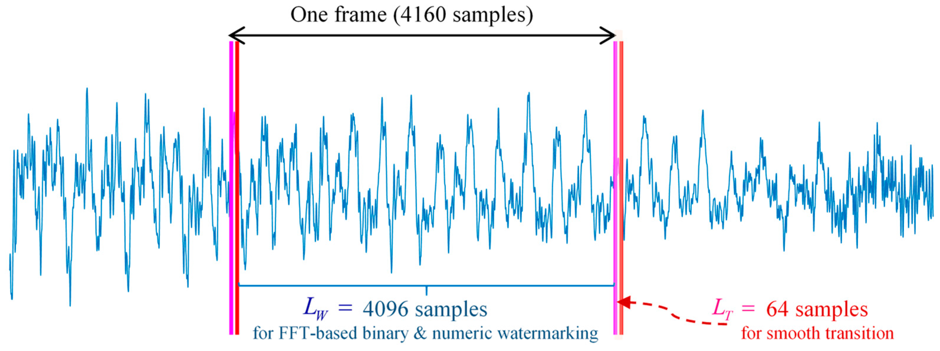
Figure 2.
Embedding procedure of the proposed FFT–PM scheme.

Figure 3.
Illustration of phase modulation (in the index range 60–107).

Figure 4.
Boundary offset adjustment in the transitional zone.

Figure 5.
Extraction procedure of the FFT–PM scheme.

Figure 6.
Color watermark images of size 64 × 64 presented in a 3 × 3 grid. Those shown on the left are scrambled versions.
Figure 6.
Color watermark images of size 64 × 64 presented in a 3 × 3 grid. Those shown on the left are scrambled versions.

Figure 7.
RMS values of the FFT magnitudes with standard error deviation bars for the first 20 Bark-scale critical bands.
Figure 7.
RMS values of the FFT magnitudes with standard error deviation bars for the first 20 Bark-scale critical bands.

Figure 8.
Histograms drawn from the original and watermarked audio signals for watermarking in four different FFT index ranges.
Figure 8.
Histograms drawn from the original and watermarked audio signals for watermarking in four different FFT index ranges.

Figure 9.
Typical watermarks (color images of size 64 × 64) extracted from the proposed FFT–PM with the FFT index range chosen as [60, 107].
Figure 9.
Typical watermarks (color images of size 64 × 64) extracted from the proposed FFT–PM with the FFT index range chosen as [60, 107].

Figure 10.
The residual network for image denoising and super-resolution reconstruction.

Figure 11.
The GAN framework for denoising and super-resolving recovered watermark images.

Figure 12.
Network architecture of the discriminator.

Figure 13.
(A–M) Examples of denoised and super-resolved images (arranged as “w64”, “BIw256”, “SR-REsNetw256”, and “SR-GANw256”) retrieved from the watermarked audio under various attacks. The label under each subpanel indicates the attack type described in Table 3.
Figure 13.
(A–M) Examples of denoised and super-resolved images (arranged as “w64”, “BIw256”, “SR-REsNetw256”, and “SR-GANw256”) retrieved from the watermarked audio under various attacks. The label under each subpanel indicates the attack type described in Table 3.

Figure 14.
Average ZNCCs derived from four sorts of watermarks in the test dataset.


Table 1.
Statistics of the measured SNRs and ODGs for the watermarks embedded in different index ranges. The data in the fourth and fifth columns are interpreted as “mean [standard deviation]”.
Table 1.
Statistics of the measured SNRs and ODGs for the watermarks embedded in different index ranges. The data in the fourth and fifth columns are interpreted as “mean [standard deviation]”.
| Embedding Scheme | FFT Index Range | Capacity [Bits/Numbers per Second] | SNR | ODG |
|---|---|---|---|---|
| AVNM | [18, 37] | 169.62 bps | 25.004 [1.650] | 0.152 [0.014] |
| PM-(I) | [49, 96] | 508.85 nps | 18.954 [2.218] | −0.095 [0.049] |
| PM-(II) | [60, 107] | 508.85 nps | 20.218 [2.216] | −0.069 [0.055] |
| PM-(III) | [72, 119] | 508.85 nps | 21.260 [2.438] | −0.065 [0.082] |
| PM-(IV) | [85, 132] | 508.85 nps | 22.314 [2.593] | −0.052 [0.099] |
| AVNM + PM-(II) | [18, 37] & [60, 107] | 169.62 bps + 508.85 nps | 18.755 [1.326] | −0.094 [0.054] |
Table 2.
Statistics of the measured entropy and correlation coefficients for the watermarks embedded in four different frequency ranges. The data in each cell are interpreted as “mean [standard deviation]”.
Table 2.
Statistics of the measured entropy and correlation coefficients for the watermarks embedded in four different frequency ranges. The data in each cell are interpreted as “mean [standard deviation]”.
| Index Range | Entropy () | Correlation Coefficient () | ||||
|---|---|---|---|---|---|---|
| Original | Watermarked | Original | Watermarked | |||
| PM-(I) | 15.041 [0.312] | 14.966 [0.256] | 0.105 [0.072] | 0.975 [0.019] | 0.975 [0.019] | 0.000 [4.9 × 10⁻⁶] |
| PM-(II) | 14.974 [0.255] | 0.096 [0.064] | 0.975 [0.019] | 0.000 [4.4 × 10⁻⁶] | ||
| PM-(III) | 14.987 [0.267] | 0.090 [0.066] | 0.975 [0.019] | 0.000 [4.2 × 10⁻⁶] | ||
| PM-(IV) | 14.984 [0.265] | 0.092 [0.067] | 0.975 [0.019] | 0.000 [4.6 × 10⁻⁶] | ||
Table 3.
Attack types and specifications.
| Item | Type | Description |
|---|---|---|
| A | Resampling | Conduct down-sampling to 22,050 Hz and then up-sampling back to 44,100 Hz. |
| B | Requantization | Quantize the watermarked signal to 8 bits/sample and then back to 16 bits/sample. |
| C | Zero thresholding | Zero out all samples below a threshold, which is set as 0.03 of the maximum dynamic range |
| D | Amplitude scaling | Scale the amplitude of the watermarked signal by 0.85. |
| E | Noise corruption (I) | Add zero-mean white Gaussian noise to the watermarked audio signal with SNR = 30 dB. |
| F | Noise corruption (II) | Add zero-mean white Gaussian noise to the watermarked audio signal with SNR = 20 dB. |
| G | Lowpass filtering | Apply a lowpass filter with a cutoff frequency of 4 kHz. |
| H | Lowpass filtering | Apply a lowpass filter with a cutoff frequency of 8 kHz. |
| I | DA/AD conversion | Convert the digital audio file to an analog signal and then resampling the analog signal at 44.1 kHz. The DA/AD conversion is performed through an onboard Realtek ALC892 audio codec, of which the line-out is linked with the line-in using a cable line during playback and recording. |
| J | Echo addition | Add an echo signal with a delay of 50 ms and a decay of 5% to the watermarked audio signal. |
| K | Jittering | Delete or add one sample randomly for every 100 samples. |
| L | MPEG-3 compression @ 128 kbps | Compress and decompress the watermarked audio signal with an MPEG layer III coder at a bit rate of 128 kbps. |
| M | MPEG-3 compression @ 64 kbps | Compress and decompress the watermarked audio signal with an MPEG layer III coder at a bit rate of 64 kbps. |
Table 4.
Average ZNCCs of the watermarks acquired from different index ranges.
| Attack Type | FFT Index Range | |||
|---|---|---|---|---|
| (I) [49, 96] | (II) [60, 107] | (III) [72, 119] | (IV) [85, 132] | |
| 0. None | 1.000 | 1.000 | 1.000 | 1.000 |
| A | 1.000 | 1.000 | 1.000 | 1.000 |
| B | 0.996 | 0.994 | 0.992 | 0.989 |
| C | 1.000 | 1.000 | 1.000 | 1.000 |
| D | 1.000 | 1.000 | 1.000 | 1.000 |
| E | 0.959 | 0.947 | 0.935 | 0.920 |
| F | 0.786 | 0.744 | 0.707 | 0.670 |
| G | 0.999 | 0.999 | 0.998 | 0.998 |
| H | 1.000 | 1.000 | 1.000 | 1.000 |
| I | 0.894 | 0.866 | 0.840 | 0.813 |
| J | 0.947 | 0.946 | 0.945 | 0.943 |
| K | 0.747 | 0.692 | 0.642 | 0.588 |
| L | 0.953 | 0.945 | 0.937 | 0.929 |
| M | 0.667 | 0.632 | 0.608 | 0.582 |
Disclaimer/Publisher’s Note: The statements, opinions and data contained in all publications are solely those of the individual author(s) and contributor(s) and not of MDPI and/or the editor(s). MDPI and/or the editor(s) disclaim responsibility for any injury to people or property resulting from any ideas, methods, instructions or products referred to in the content. |
© 2023 by the authors. Licensee MDPI, Basel, Switzerland. This article is an open access article distributed under the terms and conditions of the Creative Commons Attribution (CC BY) license (https://creativecommons.org/licenses/by/4.0/).
Share and Cite
MDPI and ACS Style
Hu, H.-T.; Lee, T.-T. Hiding Full-Color Images into Audio with Visual Enhancement via Residual Networks. Cryptography 2023, 7, 47. https://doi.org/10.3390/cryptography7040047
AMA Style
Hu H-T, Lee T-T. Hiding Full-Color Images into Audio with Visual Enhancement via Residual Networks. Cryptography. 2023; 7(4):47. https://doi.org/10.3390/cryptography7040047
Chicago/Turabian StyleHu, Hwai-Tsu, and Tung-Tsun Lee. 2023. "Hiding Full-Color Images into Audio with Visual Enhancement via Residual Networks" Cryptography 7, no. 4: 47. https://doi.org/10.3390/cryptography7040047