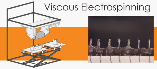
An Adaptable Device for Scalable Electrospinning of Low- and High-Viscosity Solutions


Abstract
1. Introduction
1.1. Needle-Free Electrospinning
1.2. An Ideal Electrospinning Device
1.3. Our Device
2. Materials and Methods
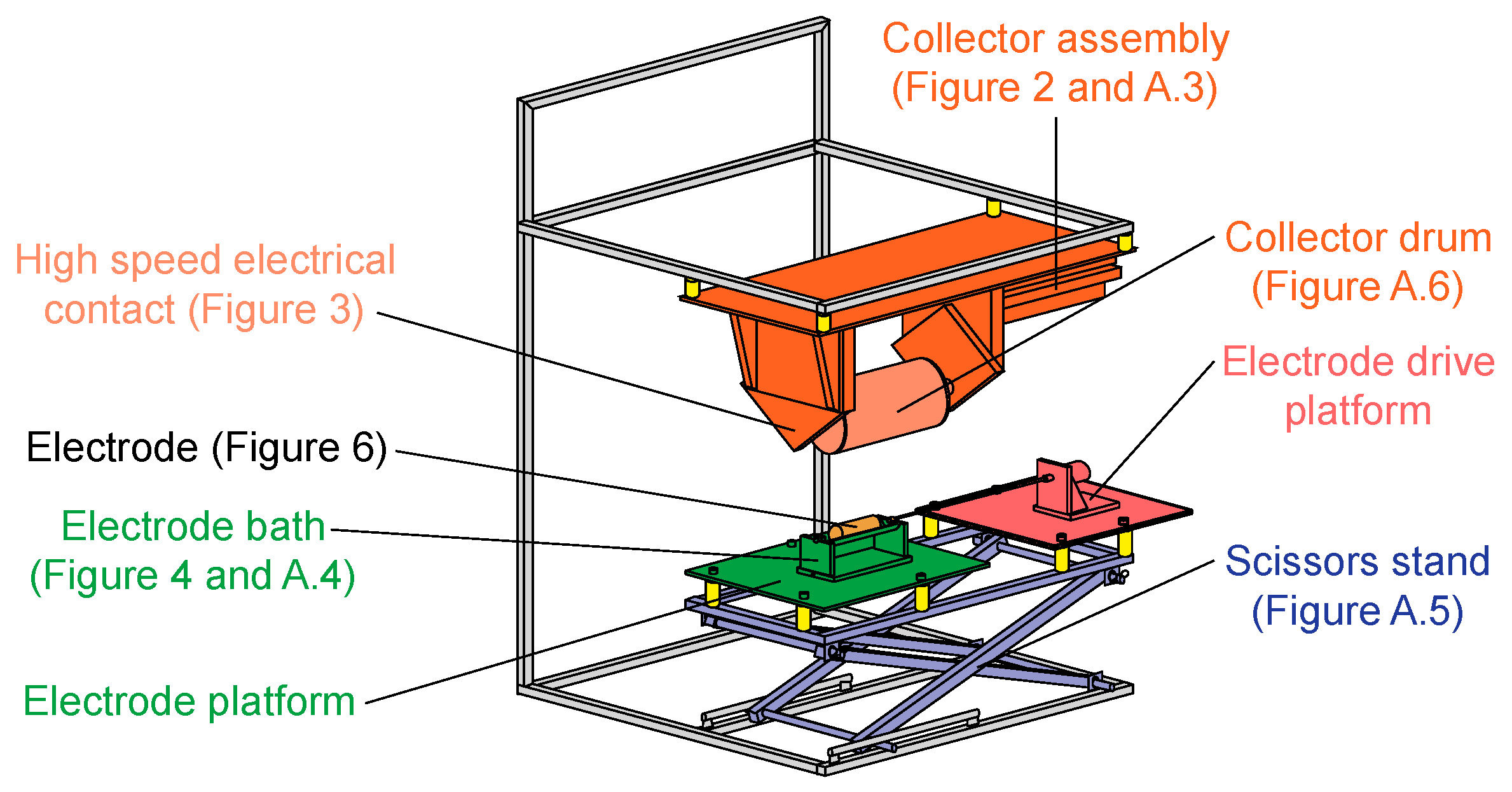
2.1. Design Overview
2.2. Frame
2.3. Dielectric Materials and Fabrication
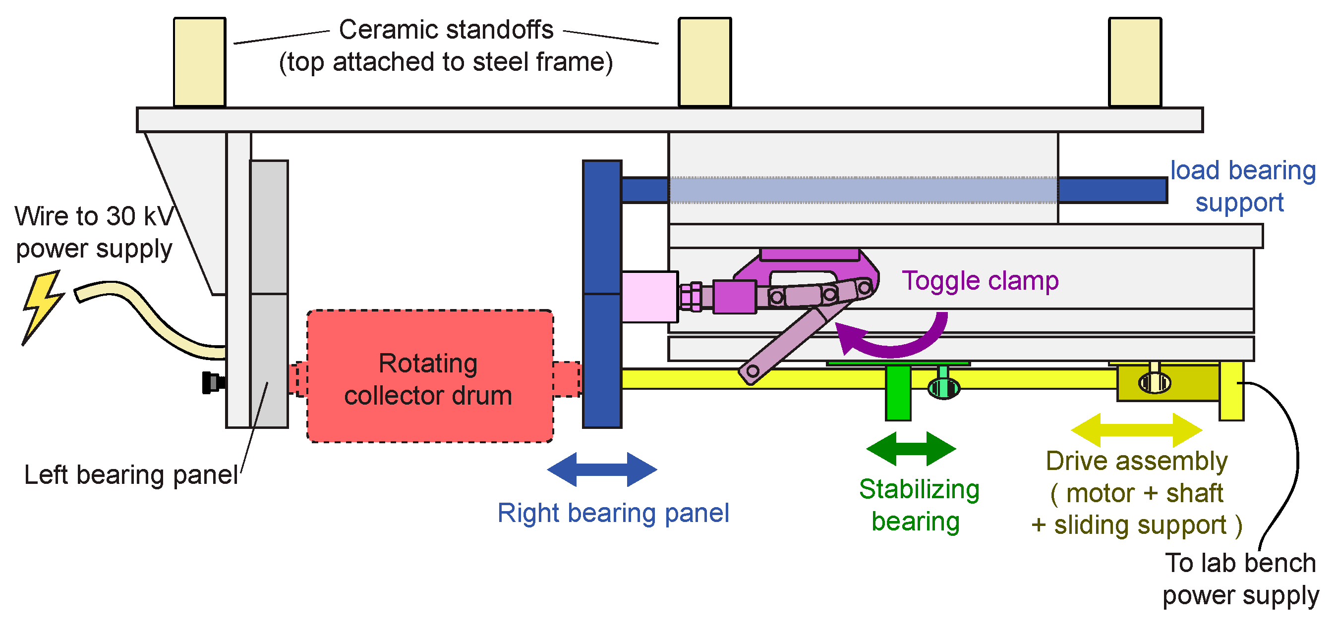
2.4. Rotating Collector Assembly
2.5. Bottom Table, Bath, and Drive Assembly
2.6. Electrodes
2.7. High-Voltage Wires
2.8. Power Supplies and Environmental Controls
2.9. Testing and Measurement
3. Results and Discussion
3.1. Results and Discussion Overview
3.2. Device Adaptability and User Interface
3.3. High-Voltage Performance
3.4. High-Voltage Safety
- De-energize the high voltage power supplies.
- Set a 5-min timer to allow the device time to discharge before opening the fume hood.
- After the timer rings, use a high-voltage grounding rod (also sold under names such as discharge stick or discharge rod) with a high-voltage insulating handle to open the fume hood doors. Then contact each part known to charge with the grounding rod tip, to ensure they had fully discharged.
3.5. Electric Field for Spinning
3.6. Mechanical Performance of Collector and Electrode
3.7. Other Design Considerations
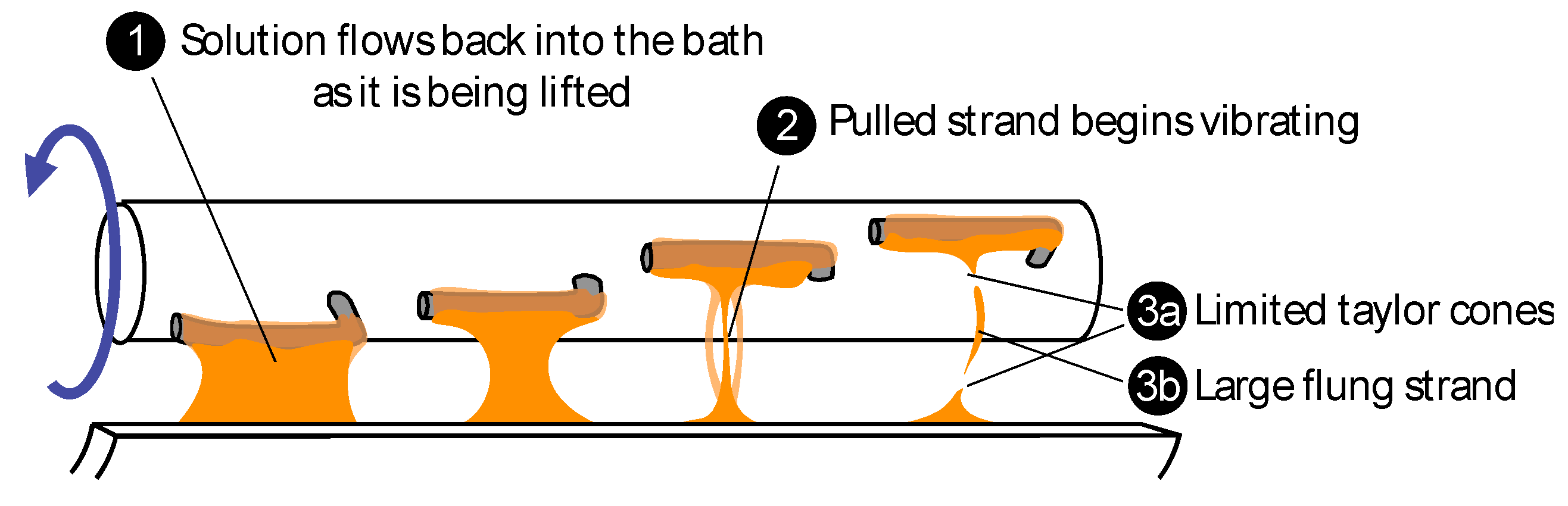
3.8. Electrode Design and Performance
3.9. Unassisted-Electrospinning Electrode Performance
3.10. Assisted Electrode Performance
4. Conclusions
Supplementary Materials
Author Contributions
Funding
Acknowledgments
Conflicts of Interest
Appendix A
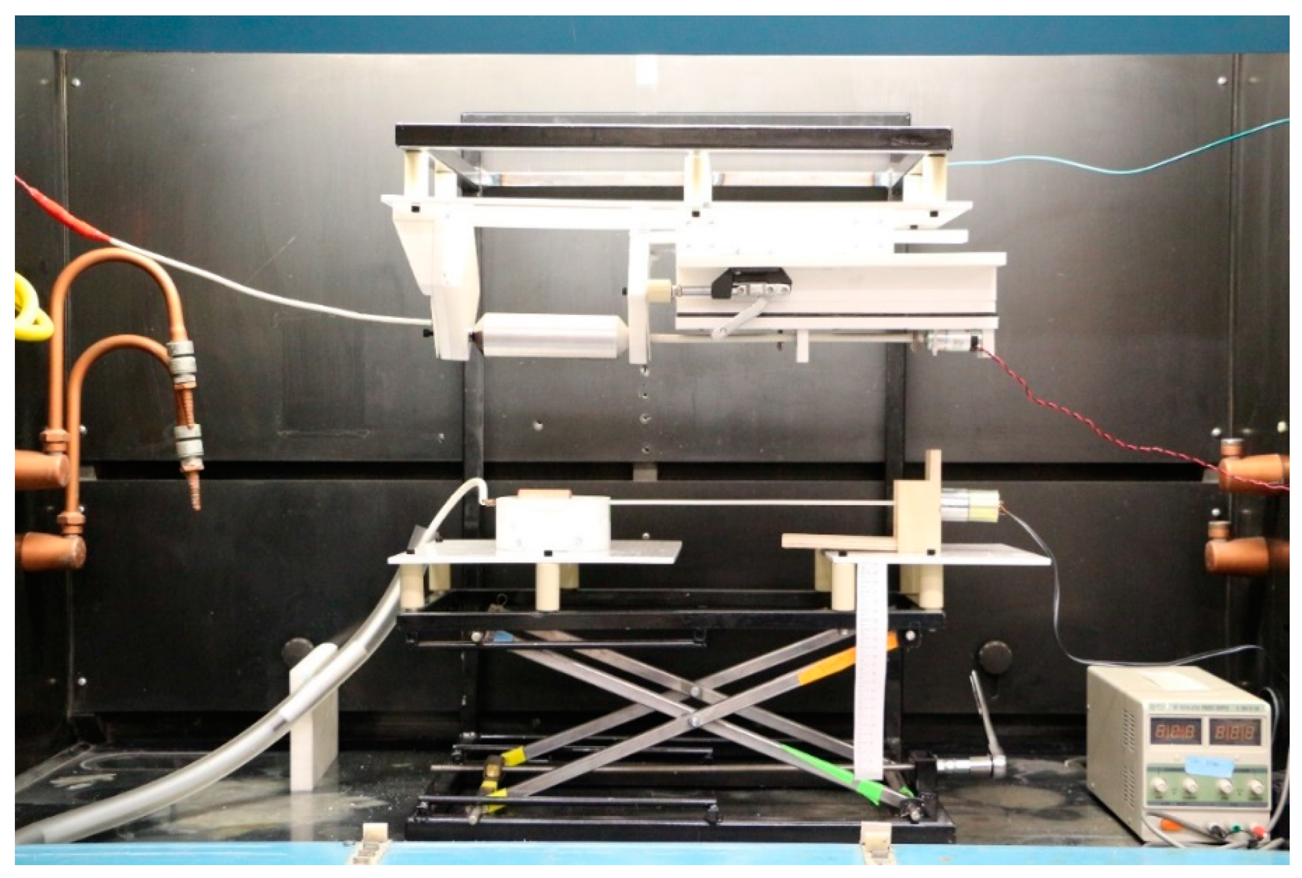
Appendix A.1. Photographs of the Device


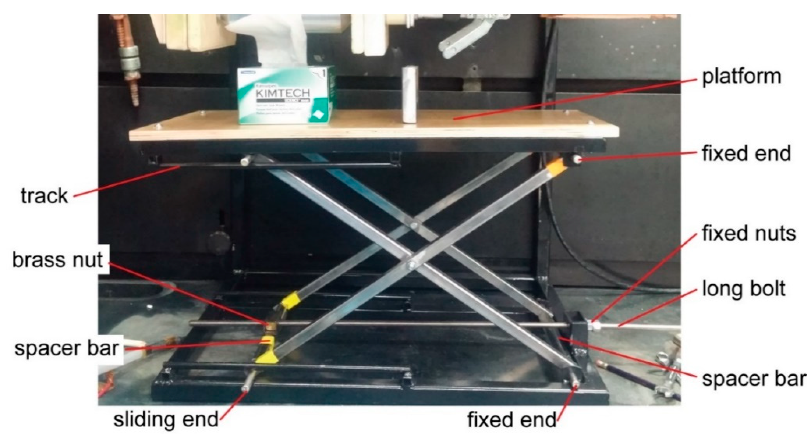
Appendix A.2. Scissors Stand Description

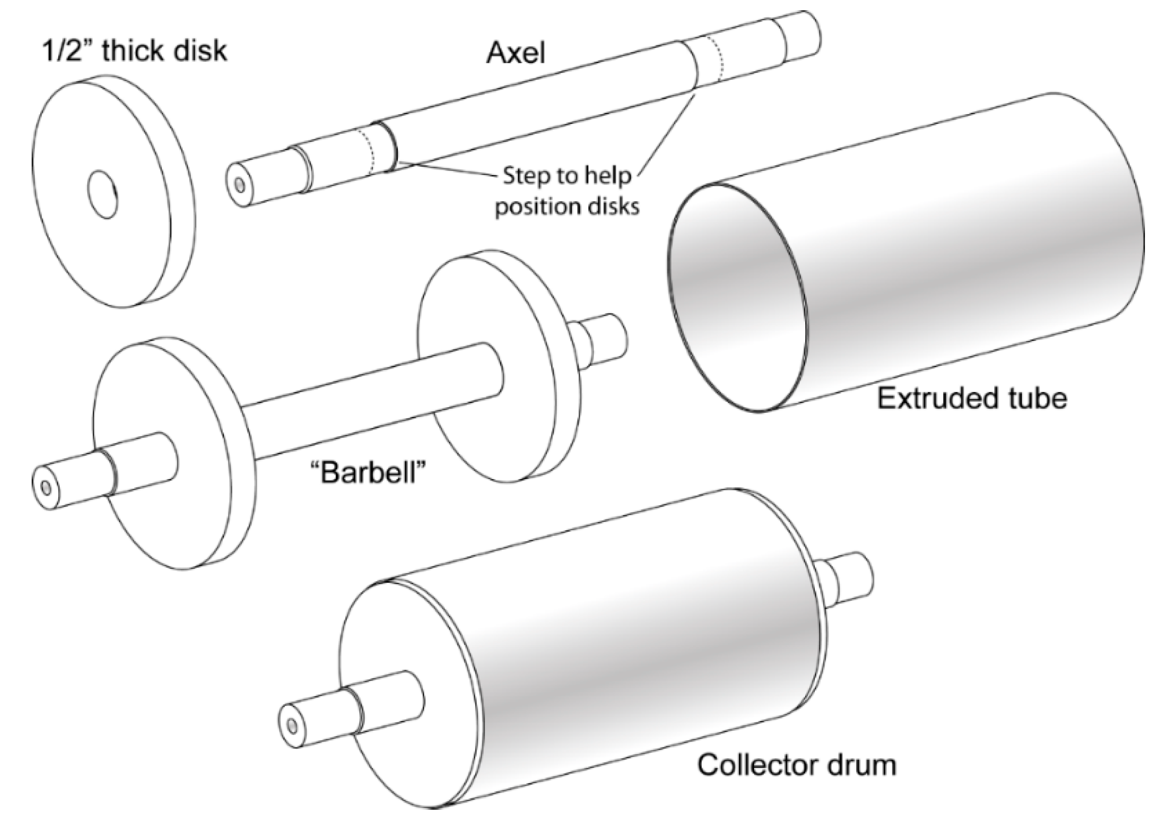
Appendix A.3. Rotating Collector Drum Fabrication

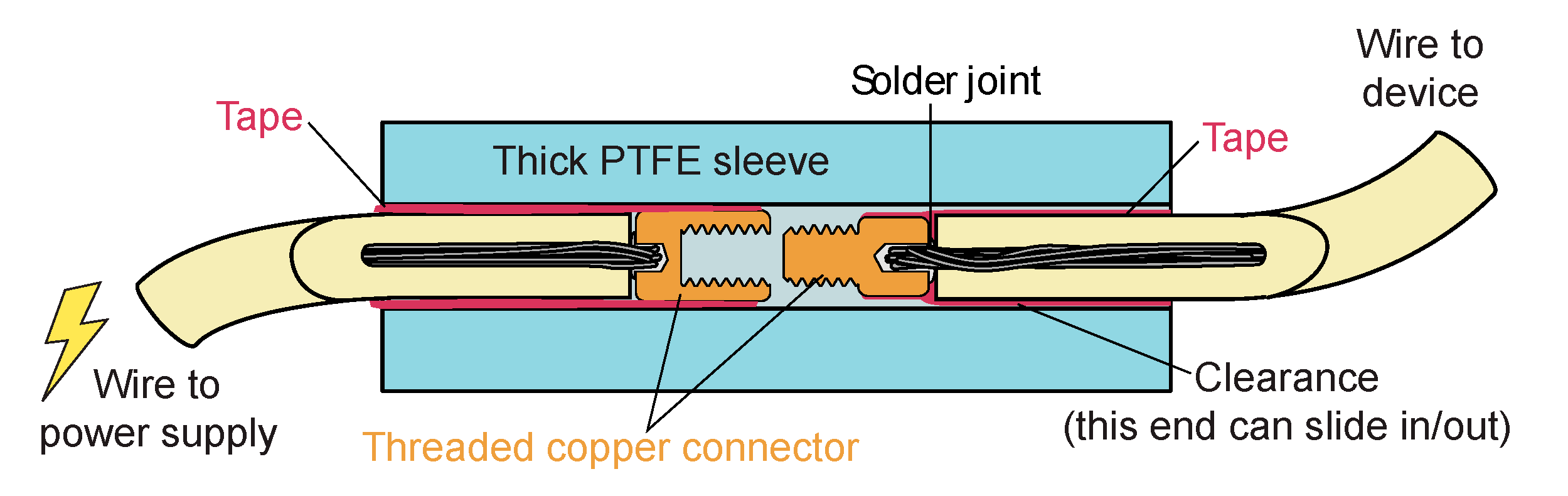
Appendix A.4. High-Voltage Connector

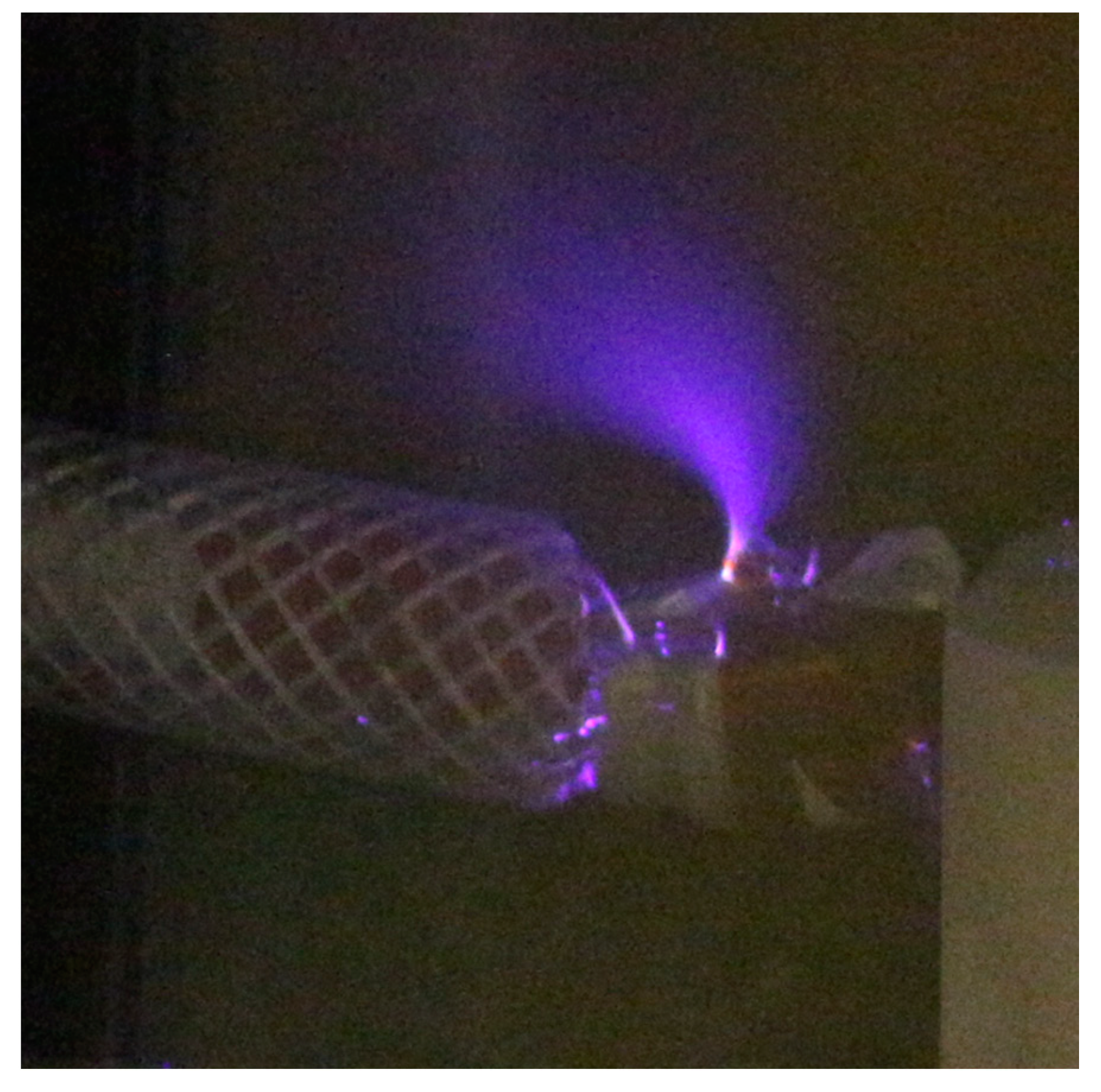
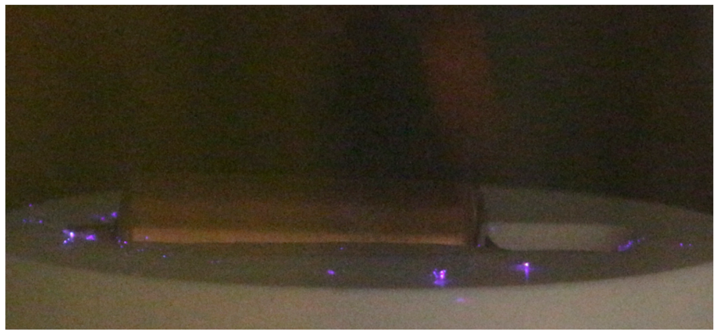
Appendix A.5. Troubleshooting Corona Discharge


Appendix A.6. Additional Electrode Designs for Taylor Cone Templating

Appendix A.7. Unsuccessful Design Concepts
Appendix A.8. Material and Time Costs
Appendix B
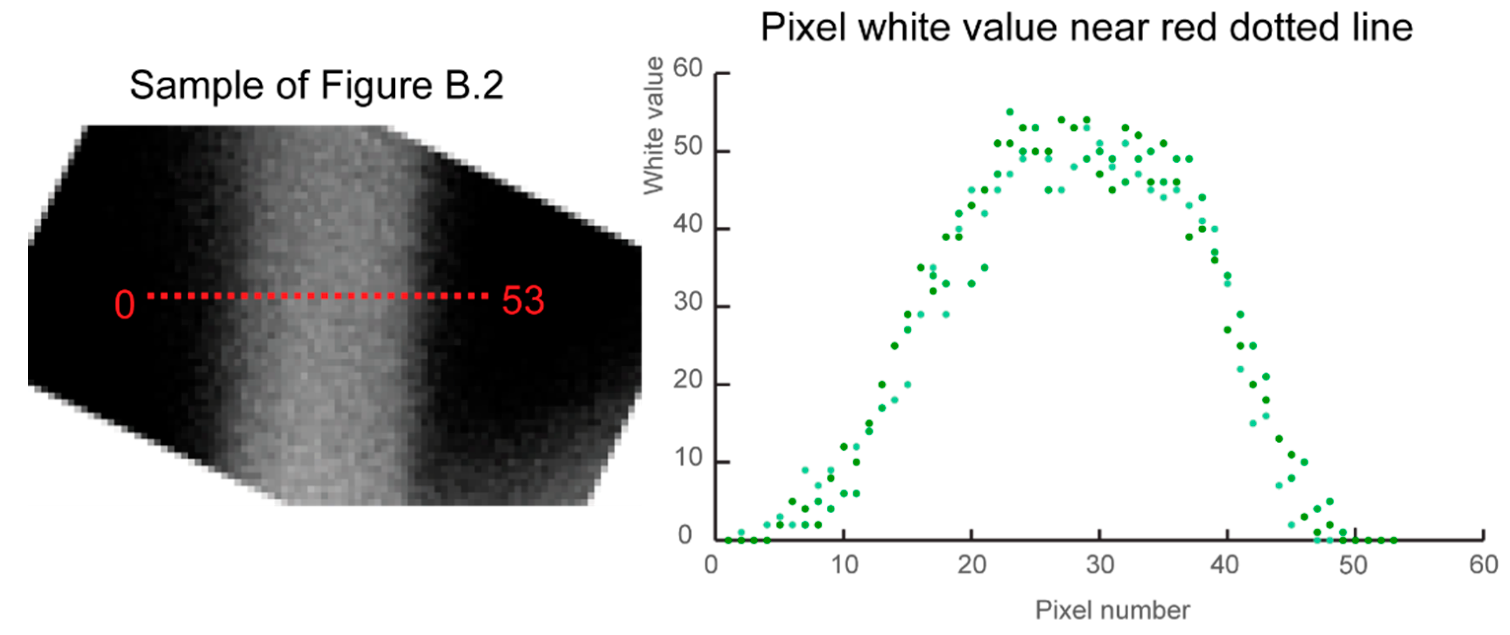
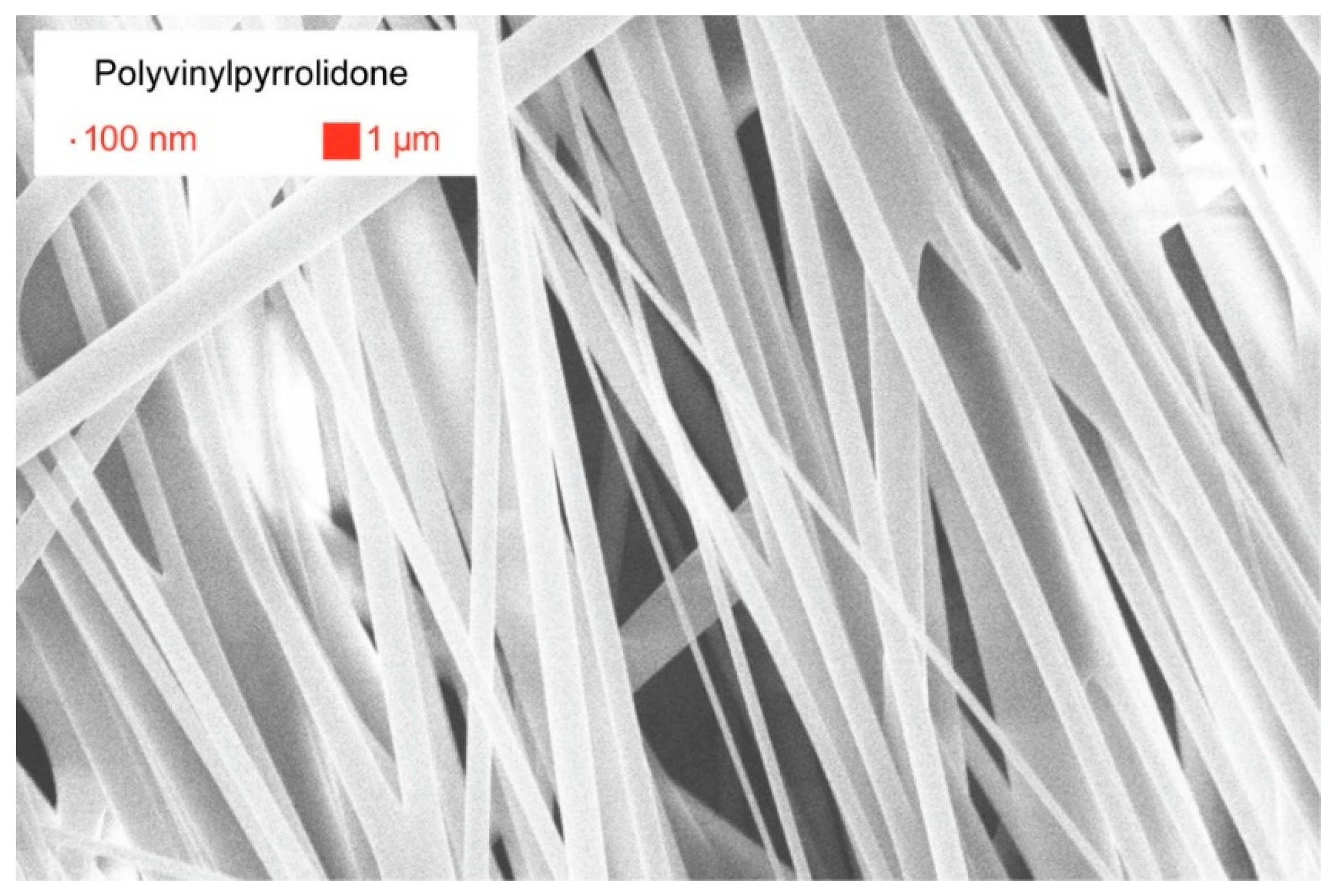
Appendix B.1. Fiber Diamater Measurments and Uncertainty Budget

| Source | Feature Size (nm) | Pixel Size (nm) | Pixel to Feature Ratio |
|---|---|---|---|
| Crouzier et al. [34] | ~29 | 2.8 | 1:10 |
| Figure A12 | 120 | 1.5 | 1:80 |
| Figure A13 | 833 | 34.5 | 1:24 |
| Figure A14 | 212 | 20.4 | 1:10 |

| Uncertainty Component Description | Estimated Uncertainty (nm) | Type | Probability Distribution | Standard Uncertainty | % Contribution |
|---|---|---|---|---|---|
| Pixel size 1 | 0.014 | B | 1σ | 0.014 | 0.0% |
| Repeatability | 0.3 | A | 1σ | 0.3 | 1.1% |
| Magnificaiton 2 | 0.26 | B | 1σ | 0.26 | 0.8% |
| Beam Width 2 | 1.7 | B | 1σ | 1.7 | 35.9% |
| Operator selection 2 | 0.2 | B | 1σ | 0.2 | 0.5% |
| Operating voltage | 2 | B | Rect. | 1.1547 | 16.6% |
| Contrast-Brightness | 1.21 | A | 1σ | 1.21 | 18.2% |
| Fiber edge | 1.04 | A | 1σ | 1.04 | 13.4% |
| Human-power | 0.29 | A | 1σ | 0.29 | 1.0% |
| Platinum coating | 1 | B | 1σ | 1 | 12.4% |
| Combined Uncertainty: | 2.8 | ||||
| k (Coverage Factor): | 2.87 | ||||
| Expanded Uncertainty: | 8.1 | ||||
| Uncertainty Component Description | Estimated Uncertainty (nm) | Type | Probability Distribution | Standard Uncertainty | % Contribution |
|---|---|---|---|---|---|
| Pixel size 1 | 0.014 | B | 1σ | 0.014 | 0.0% |
| Repeatability | 0.3 | A | 1σ | 0.3 | 0.1% |
| Magnificaiton 2 | 0.26 | B | 1σ | 0.26 | 0.1% |
| Beam Width 2 | 1.7 | B | 1σ | 1.7 | 2.2% |
| Operator selection 2 | 0.2 | B | 1σ | 0.2 | 0.0% |
| Operating voltage | 2 | B | Rect. | 1.1547 | 1.0% |
| Contrast-Brightness | 8.4133 | A | 1σ | 8.4133 | 53.3% |
| Fiber edge | 7.2471 | A | 1σ | 7.2471 | 39.6% |
| Human-power | 1.9992 | A | 1σ | 1.9992 | 3.0% |
| Platinum coating | 1 | B | 1σ | 1 | 0.8% |
| Combined Uncertainty: | 11.5 | ||||
| k (Coverage Factor): | 4.5 | ||||
| Expanded Uncertainty: | 52.2 | ||||
| Uncertainty Component Description | Estimated Uncertainty (nm) | Type | Probability Distribution | Standard Uncertainty | % Contribution |
|---|---|---|---|---|---|
| Pixel size 1 | 0.014 | B | 1σ | 0.014 | 0.0% |
| Repeatability | 0.3 | A | 1σ | 0.3 | 0.7% |
| Magnificaiton 2 | 0.26 | B | 1σ | 0.26 | 0.5% |
| Beam Width 2 | 1.7 | B | 1σ | 1.7 | 21.1% |
| Operator selection 2 | 0.2 | B | 1σ | 0.2 | 0.3% |
| Operating voltage | 2 | B | Rect. | 1.1547 | 9.8% |
| Contrast-Brightness | 2.1412 | A | 1σ | 2.1412 | 33.5% |
| Fiber edge | 1.8444 | A | 1σ | 1.8444 | 24.9% |
| Human-power | 0.5088 | A | 1σ | 0.5088 | 1.9% |
| Platinum coating | 1 | B | 1σ | 1 | 7.3% |
| Combined Uncertainty: | 3.7 | ||||
| k (Coverage Factor): | 2.87 | ||||
| Expanded Uncertainty: | 10.6 | ||||
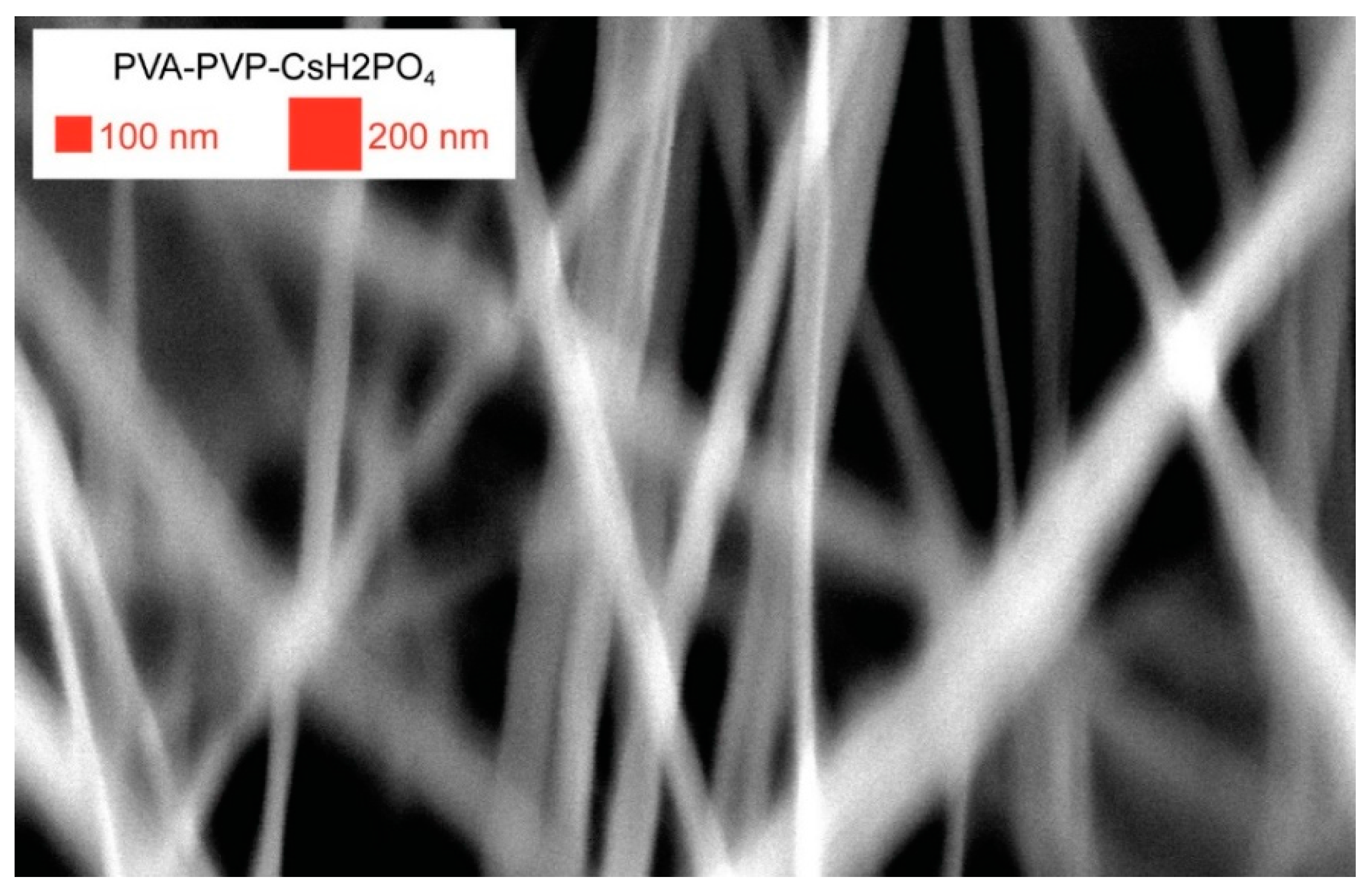
Appendix B.2. Demonstration on Select Compositions


Appendix B.3. System Paramaters
| Parameter | Minimum | Maximum | Units |
|---|---|---|---|
| Total bias | 0 | 93,000 1 | volts |
| Collector electrode distance at peak voltage | 11 | 33 | cm |
| Electrode rotational frequency | 0.03 | 0.2 | Hz |
| Electrode rotational frequency | 2 | 12 | rpm |
| Collector rotational frequency | 0 | 105 | Hz |
| Collector rotational frequency | 0 | 6300 | rpm |
| Collector surface speed | 0 | 50 | m/s |
| Parameter | Minimum | Maximum | Units | Source |
|---|---|---|---|---|
| Air temperature | 19 | 55 | C | External air heaters |
| Air flow | 0 1 | 0.6 | m/s | Fans and fume hood |
| Relative humidity | 15 2 | 85 | % | Dehumidifier or humidifiers |
References
- Saldanha, P.L.; Lesnyak, V.; Manna, L. Large scale syntheses of colloidal nanomaterials. Nano Today 2017, 12, 46–63. [Google Scholar] [CrossRef]
- Niu, H.; Lin, T. Fiber generators in needleless electrospinning. J. Nanomater. 2012, 2012. [Google Scholar] [CrossRef]
- Haider, A.; Haider, S.; Kang, I.K. A comprehensive review summarizing the effect of electrospinning parameters and potential applications of nanofibers in biomedical and biotechnology. Arab. J. Chem. 2018, 11, 1165–1188. [Google Scholar] [CrossRef]
- Ray, S.S.; Chen, S.S.; Li, C.W.; Nguyen, N.C.; Nguyen, H.T. A comprehensive review: Electrospinning technique for fabrication and surface modification of membranes for water treatment application. RSC Adv. 2016, 6, 85495–85514. [Google Scholar] [CrossRef]
- Aruna, S.T.; Balaji, L.S.; Kumar, S.S.; Prakash, B.S. Electrospinning in solid oxide fuel cells—A review. Renew. Sustain. Energy Rev. 2017, 67, 673–682. [Google Scholar] [CrossRef]
- Xu, J.; Liu, C.; Hsu, P.C.; Liu, K.; Zhang, R.; Liu, Y.; Cui, Y. Roll-to-Roll Transfer of Electrospun Nanofiber Film for High-Efficiency Transparent Air Filter. Nano Lett. 2016, 16, 1270–1275. [Google Scholar] [CrossRef]
- ElectrospinTech Contributiors. ElectrospinTech. Available online: http://electrospintech.com/ (accessed on 10 March 2019).
- Taylor, G. Disintegration of water drops in an electric field. Proc. R. Soc. Lond. Ser. A Math. Phys. Sci. 1964, 280, 383–397. [Google Scholar] [CrossRef]
- Ryan, C.N.; Smith, K.L.; Stark, J.P.W. Characterization of multi-jet electrospray systems. J. Aerosol Sci. 2012, 51, 35–48. [Google Scholar] [CrossRef]
- Amariei, N.; Manea, L.R.; Bertea, A.P.; Bertea, A.; Popa, A. The Influence of Polymer Solution on the Properties of Electrospun 3D Nanostructures. IOP Conf. Ser. Mater. Sci. Eng. 2017, 209. [Google Scholar] [CrossRef]
- Tiwari, S.K.; Venkatraman, S.S. Importance of viscosity parameters in electrospinning: Of monolithic and core-shell fibers. Mater. Sci. Eng. C 2012, 32, 1037–1042. [Google Scholar] [CrossRef]
- Al-Mezrakchi, R.Y.H.; Naraghi, M. Interfused nanofibres network in scalable manufacturing of polymeric fibres via multi-nozzle electrospinning. Micro Nano Lett. 2018, 13, 536–540. [Google Scholar] [CrossRef]
- Rodoplu, D.; Mutlu, M. Effects of Electrospinning Setup and Process Parameters on Nanofiber Morphology Intended for the Modification of Quartz Crystal Microbalance Surfaces. J. Eng. Fiber. Fabr. 2012, 7, 155892501200700. [Google Scholar] [CrossRef]
- Dias, J.R.; Dos Santos, C.; Horta, J.; Granja, P.L.; Bartolo, P.J.D.S. A new design of an electrospinning apparatus for tissue engineering applications. Int. J. Bioprint. 2017, 3, 121–129. [Google Scholar] [CrossRef]
- Jirsak, O.; Sanetrnik, F.; Lukas, D.; Kotek, V.; Martinova, L.; Chaloupek, J. Způsob Výroby Nanovláken z Polymerního Roztoku Elektrostatickým Zvlákňováním a Zařízení k Provádění Způsobu. CZ294274B6, 8 September 2003. [Google Scholar]
- Wei, L.; Qiu, Q.; Wang, R.; Qin, X. Influence of the processing parameters on needleless electrospinning from double ring slits spinneret using response surface methodology. J. Appl. Polym. Sci. 2018, 135, 1–8. [Google Scholar] [CrossRef]
- Yan, G.; Niu, H.; Zhou, H.; Wang, H.; Shao, H.; Zhao, X.; Lin, T. Electro-aerodynamic field aided needleless electrospinning. Nanotechnology 2018, 29. [Google Scholar] [CrossRef] [PubMed]
- Yalcinkaya, F. Preparation of various nanofiber layers using wire electrospinning system. Arab. J. Chem. 2016. [Google Scholar] [CrossRef]
- Wang, X.; Lin, T.; Wang, X. Use of airflow to improve the nanofibrous structure and quality of nanofibers from needleless electrospinning. J. Ind. Text. 2015, 45, 310–320. [Google Scholar] [CrossRef]
- Ali, U.; Niu, H.; Aslam, S.; Jabbar, A.; Rajput, A.W.; Lin, T. Needleless electrospinning using sprocket wheel disk spinneret. J. Mater. Sci. 2017, 52, 7567–7577. [Google Scholar] [CrossRef]
- Jiang, G.; Zhang, S.; Wang, Y.; Qin, X. An improved free surface electrospinning with micro-bubble solution system for massive production of nanofibers. Mater. Lett. 2015, 144, 22–25. [Google Scholar] [CrossRef]
- Niu, H.; Wang, X.; Lin, T. Needleless electrospinning: Influences of fibre generator geometry. J. Text. Inst. 2012, 103, 787–794. [Google Scholar] [CrossRef]
- Zheng, Y.S.; Xie, S.; Zeng, Y.C. Effects of Structural Parameters on Nanofiber from a Multihole Electrospinning Setup. Adv. Mater. Res. 2013, 690–693, 2886–2890. [Google Scholar] [CrossRef]
- Thoppey, N.M.; Gorga, R.E.; Bochinski, J.R.; Clarke, L.I. Effect of solution parameters on spontaneous jet formation and throughput in edge electrospinning from a fluid-filled bowl. Macromolecules 2012, 45, 6527–6537. [Google Scholar] [CrossRef]
- He, H.J.; Liu, C.K.; Molnar, K. A Novel Needleless Electrospinning System Using a Moving Conventional Yarn as the Spinneret. Fibers Polym. 2018, 19, 1472–1478. [Google Scholar] [CrossRef]
- Um, I.C.; Fang, D.; Hsiao, B.S.; Okamoto, A.; Chu, B. Electro-spinning and electro-blowing of hyaluronic acid. Biomacromolecules 2004, 5, 1428–1436. [Google Scholar] [CrossRef] [PubMed]
- Varabhas, J.S.; Tripatanasuwan, S.; Chase, G.G.; Reneker, D.H. Electrospun jets launched from polymeric bubbles. J. Eng. Fiber. Fabr. 2009, 4, 46–50. [Google Scholar] [CrossRef]
- Wu, D.; Xiao, Z.; Deng, L.; Sun, Y.; Tan, Q.; Dong, L.; Huang, S.; Zhu, R.; Liu, Y.; Zheng, W.; et al. Enhanced Deposition Uniformity via an Auxiliary Electrode in Massive Electrospinning. Nanomaterials 2016, 6, 135. [Google Scholar] [CrossRef]
- Wu, D.; Deng, L.; Sun, Y.; Teh, K.S.; Shi, C.; Tan, Q.; Zhao, J.; Sun, D.; Lin, L. A high-safety PVDF/Al2O3 composite separator for Li-ion batteries via tip-induced electrospinning and dip-coating. RSC Adv. 2017, 7, 24410–24416. [Google Scholar] [CrossRef]
- Curry, K.; Zubiate, B.; Sanghrajka, A.; Aslamaci, A.; Mortimer, C.; Ladd, M.R.; Zhang, X. Post on “Charging a Rotating Mandrel Collector for Electrospinning?”. Available online: https://www.researchgate.net/post/Charging_a_rotating_mandrel_collector_for_electrospinning (accessed on 18 January 2018).
- Jentzsch, E.; Gül, Ö.; Öznergiz, E. A comprehensive electric field analysis of a multifunctional electrospinning platform. J. Electrostat. 2013, 71, 294–298. [Google Scholar] [CrossRef]
- Fan, Z.-Z.; He, H.-W.; Yan, X.; Zhao, R.-H.; Long, Y.-Z.; Ning, X. Fabrication of Ultrafine PPS Fibers with High Strength and Tenacity via Melt Electrospinning. Polymers 2019, 11, 530. [Google Scholar] [CrossRef]
- Rosell-Llompart, J.; Grifoll, J.; Loscertales, I.G. Electrosprays in the cone-jet mode: From Taylor cone formation to spray development. J. Aerosol Sci. 2018, 125, 2–31. [Google Scholar] [CrossRef]
- Crouzier, L.; Delvallee, A.; Allard, A.; Devoille, L.; Ducourtieux, S.; Feltin, N. Methodology to evaluate the uncertainty associated with nanoparticle dimensional measurements by SEM. Meas. Sci. Technol. 2019. [Google Scholar] [CrossRef]
- The Joint Committee for Guides in Metrology. JCGM 100: 2008, Guide to the Expression of Uncertainty in Measurement, GUM 1995 with Minor Corrections; International Bureau of Weights and Measures: Paris, France, 2008. [Google Scholar]
- Hotaling, N.A.; Bharti, K.; Kriel, H.; Simon, C.G. DiameterJ: A validated open source nanofiber diameter measurement tool. Biomaterials 2015, 61, 327–338. [Google Scholar] [CrossRef] [PubMed]
- Hotaling, N.A.; Bharti, K.; Kriel, H.; Simon, C.G. Dataset for the validation and use of DiameterJ an open source nanofiber diameter measurement tool. Data Brief 2015, 5, 13–22. [Google Scholar] [CrossRef] [PubMed]
- Öznergiz, E.; Kiyak, Y.E.; Kamasak, M.E.; Yildirim, I. Automated nanofiber diameter measurement in SEM images using a robust image analysis method. J. Nanomater. 2014, 2014. [Google Scholar] [CrossRef]
- Delvallée, A.; Feltin, N.; Ducourtieux, S.; Trabelsi, M.; Hochepied, J.F. Direct comparison of AFM and SEM measurements on the same set of nanoparticles. Meas. Sci. Technol. 2015, 26. [Google Scholar] [CrossRef]
- Radacsi, N.; Campos, F.D.; Chisholm, C.R.I.; Giapis, K.P. Spontaneous formation of nanoparticles on electrospun nanofibres. Nat. Commun. 2018, 9, 3–10. [Google Scholar] [CrossRef] [PubMed]
- Goñi-Urtiaga, A.; Scott, K.; Cavaliere, S.; Jones, D.J.; Roziére, J. A new fabrication method of an intermediate temperature proton exchange membrane by the electrospinning of CsH2PO4. J. Mater. Chem. A 2013, 1, 10875. [Google Scholar] [CrossRef]
- Kim, Y.; Lee, D.-Y.; Lee, M.-H.; Lee, S.-J. Electrospun Calcium Metaphosphate Nanofibers: I. Fabrication. J. Korean Ceram. Soc. 2007, 44, 144–147. [Google Scholar] [CrossRef]
- Tadjiev, T.R.; Chun, S.S.; Kim, H.M.; Kang, I.K.; Kim, S.Y. Preparation and Characterization of β-Tricalcium Phosphate Nanofibers via Electrospinning. Key Eng. Mater. 2009, 342–343, 817–820. [Google Scholar] [CrossRef]


© 2019 by the authors. Licensee MDPI, Basel, Switzerland. This article is an open access article distributed under the terms and conditions of the Creative Commons Attribution (CC BY) license (http://creativecommons.org/licenses/by/4.0/).
Share and Cite
McCarty, R.J.; Giapis, K.P. An Adaptable Device for Scalable Electrospinning of Low- and High-Viscosity Solutions. Instruments 2019, 3, 37. https://doi.org/10.3390/instruments3030037
McCarty RJ, Giapis KP. An Adaptable Device for Scalable Electrospinning of Low- and High-Viscosity Solutions. Instruments. 2019; 3(3):37. https://doi.org/10.3390/instruments3030037
Chicago/Turabian StyleMcCarty, Ryan J., and Konstantinos P. Giapis. 2019. "An Adaptable Device for Scalable Electrospinning of Low- and High-Viscosity Solutions" Instruments 3, no. 3: 37. https://doi.org/10.3390/instruments3030037
APA StyleMcCarty, R. J., & Giapis, K. P. (2019). An Adaptable Device for Scalable Electrospinning of Low- and High-Viscosity Solutions. Instruments, 3(3), 37. https://doi.org/10.3390/instruments3030037