
Design and Development of a High-Accuracy IoT System for Real-Time Load and Space Monitoring in Shipping Containers


Abstract
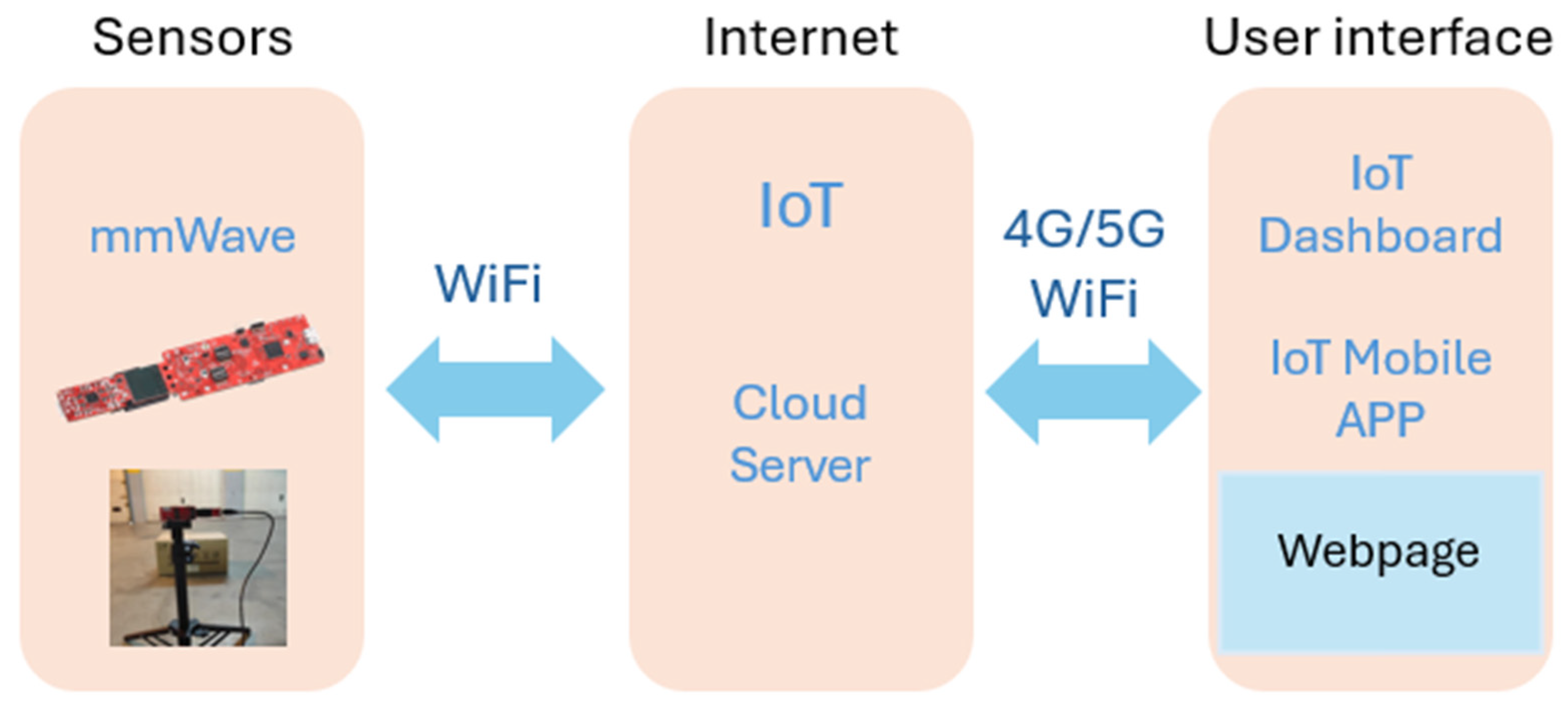
1. Introduction
2. Background and State of the Art
2.1. Background of Object Detection Technologies
- They do not rely on visible light like other types of technology, allowing them to be used in both indoor and outdoor environments without concerns about environmental conditions affecting performance levels;
- They have self-diagnostic capabilities, providing users with quick access to the collected information [9].
2.2. State of the Art: mmWave Technology
3. Materials and Methods
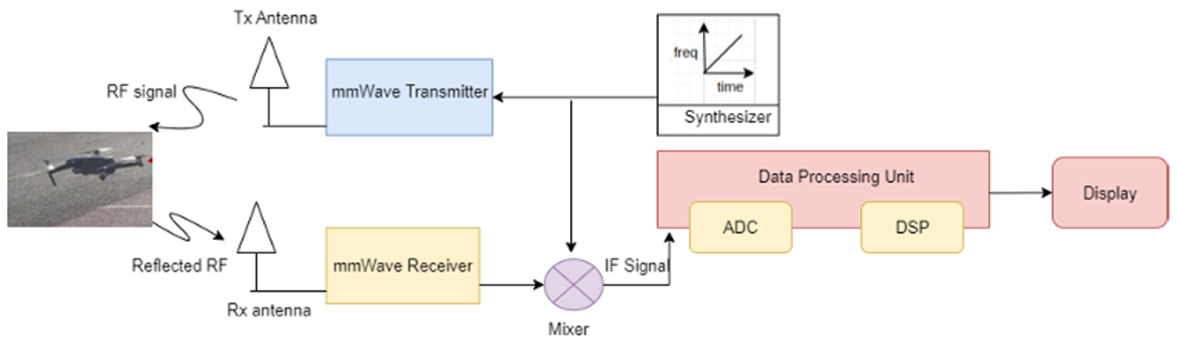
3.1. Underlying Theory FMCW
- c is the speed of light ();
- is the frequency difference (beat frequency);
- is the frequency slope of the chirp.
- d is the distance between antennas in the array;
- λ is the wavelength of the signal;
- θ is the AoA.
- xmim = −Rx/2 and xmax = Rx/2 (where the origin is in the center of the volume and the length is Rx);
- ymim = −Ry/2 and ymax = Ry/2 (where the origin is in the center of the volume and the length is Ry);
- zmim = 0 and zmax = Rz (with the ground as reference, z = 0).
| Algorithm 1. For IWR6843 |
| Function DBSCAN(Points, ε, MinPts) Clusters ← [], Volumes ← [] For each unvisited point P do Mark P as visited, Neighbors ← {Q | Distance(P, Q) ≤ ε} If size(Neighbors) < MinPts then continue Cluster ← Expand(P, Neighbors, Points, ε, MinPts) Add Cluster to Clusters For each Cluster in Clusters do Volumes ← Volumes + ComputeVolume(ConvexHull(Cluster)) Return Clusters, Volumes End Function Function Expand(P, Neighbors, Points, ε, MinPts) Cluster ← {P} For each Q in Neighbors do If Q is not visited then Mark Q as visited, NewNeighbors ← {R | Distance(Q, R) ≤ ε} If size(NewNeighbors) ≥ MinPts then Neighbors ← Neighbors ∪ NewNeighbors Add Q to Cluster Return Cluster End Function Function ComputeVolume(Hull) Return |Σ Determinant(Origin, A, B, C)/6 for each (A, B, C) in Hull| End Function |
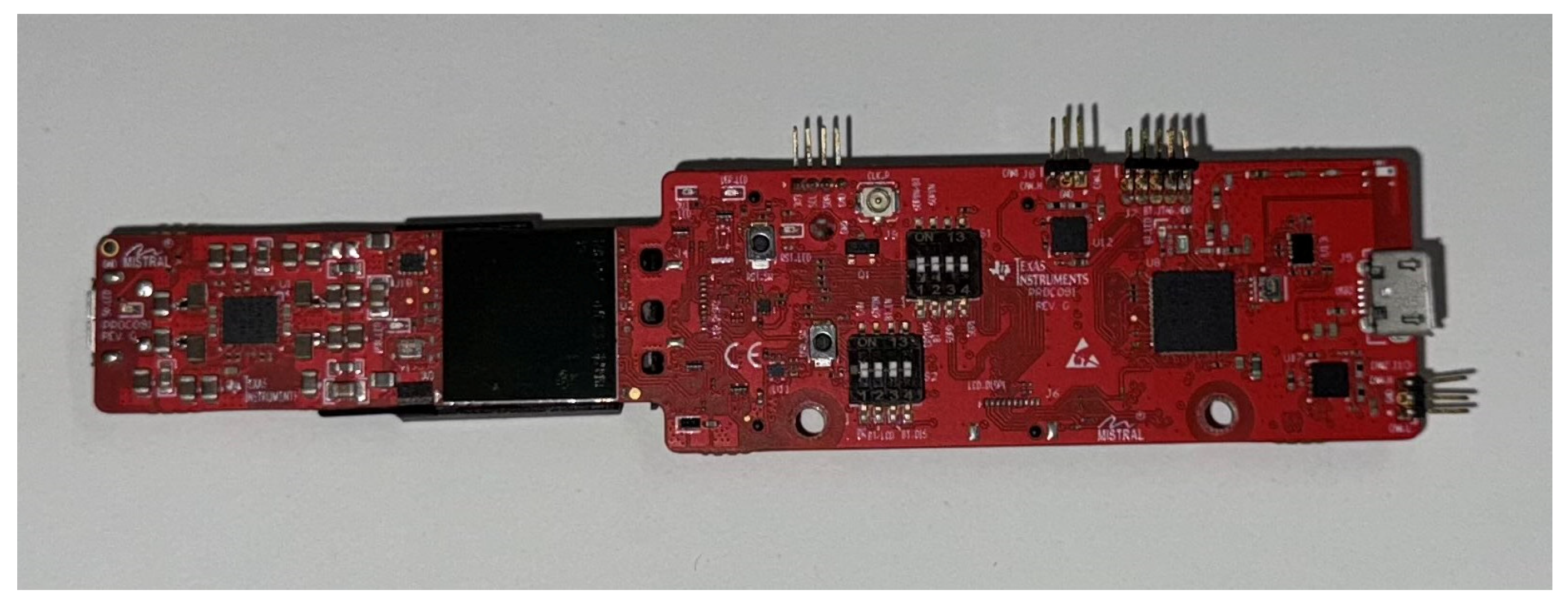
3.2. Practical Operation of the IWR6843
- A high-performance TI C674x DSP subsystem for advanced radar signal processing, magnitude, detection, and many other applications.
- A Built-In Self-Test (BIST) processor subsystem, responsible for radio configuration, control, and calibration.
- A user-programmable ARM Cortex-R4F for object detection and interface control;
- Three antennas for TX and four antennas for RX.
- A PLL, transmitter, receiver, and ADC.
- A single cable for power and data.
- Coverage from 60 to 64 GHz with a continuous bandwidth of 4 GHz.
- A hardware accelerator for FFT, filtering, and Constant False Alarm Rate (CFAR) processing.
- Up to six ADC channels, up to two Serial Peripheral Interface (SPI) ports, up to two UART ports, Inter-Integrated Circuit (I2C), and a Low Voltage Differential Signaling (LVDS) interface.
- Azimuth Field Of View (FOV) +/− 60 degrees, with an angular resolution of 29 degrees.
- Elevation FOV +/− 60 degrees, with an angular resolution of 29 degrees.
- This device enables a vast variety of applications with simple changes to the programming model. Additionally, it offers the possibility of dynamic reconfiguration, meaning in real-time and while in operation, to implement a multimodal sensor.
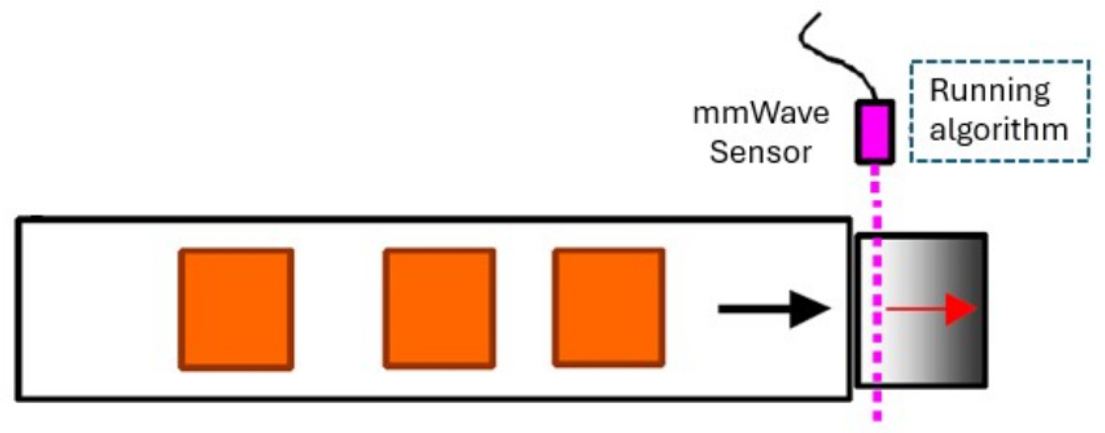
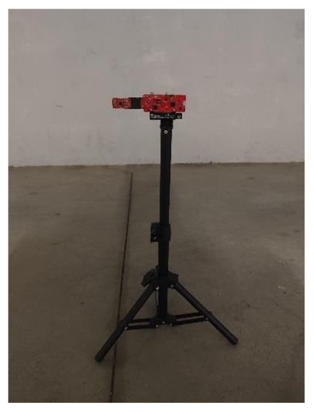
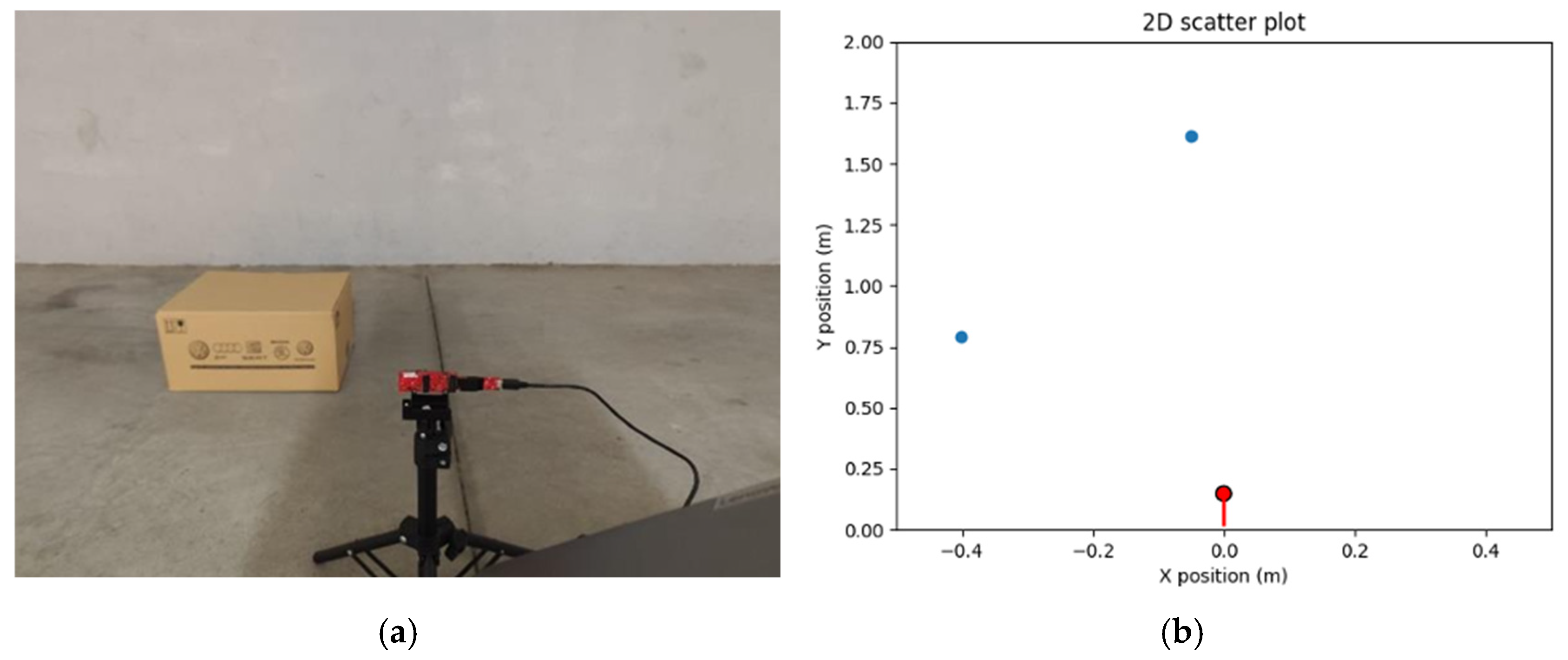
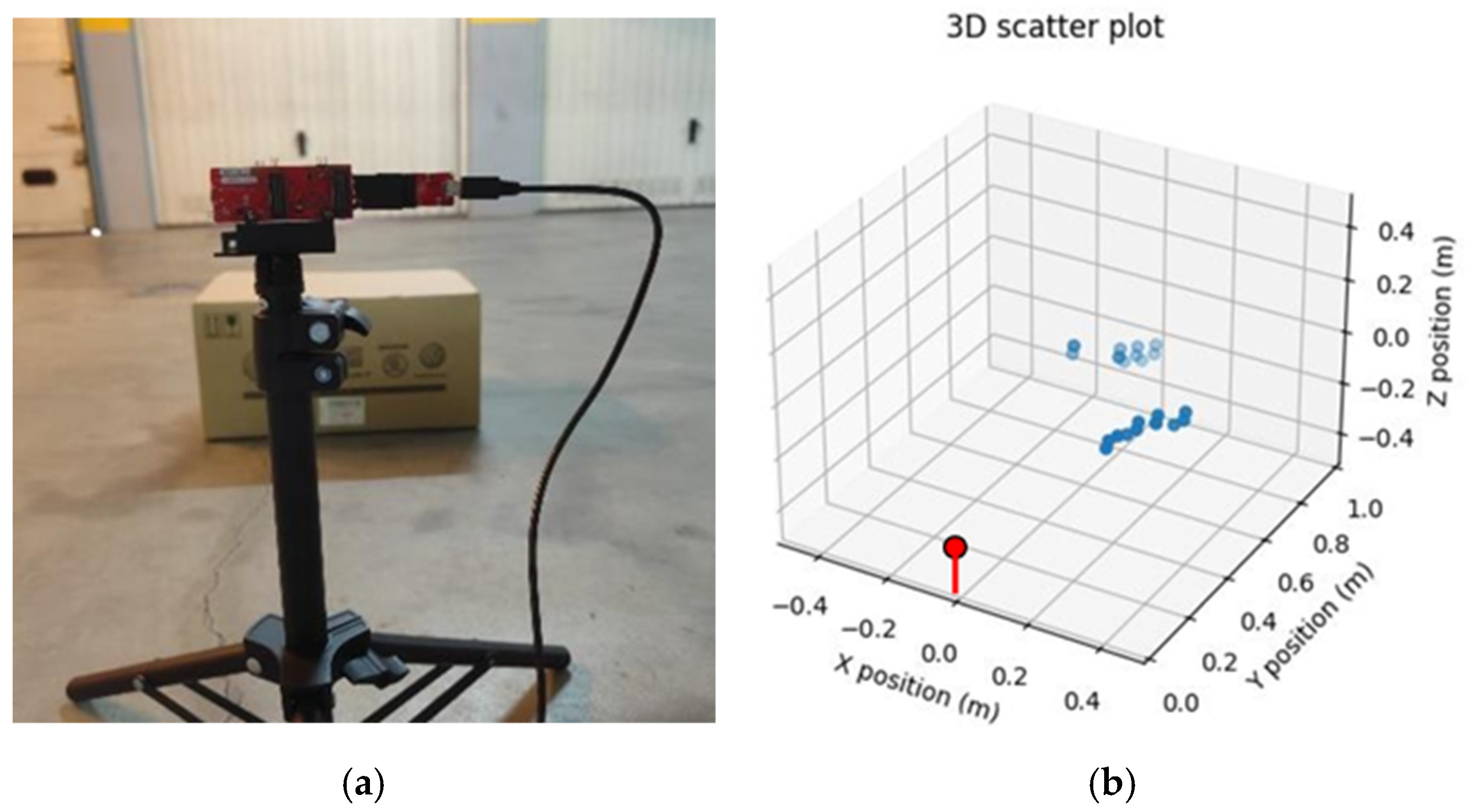
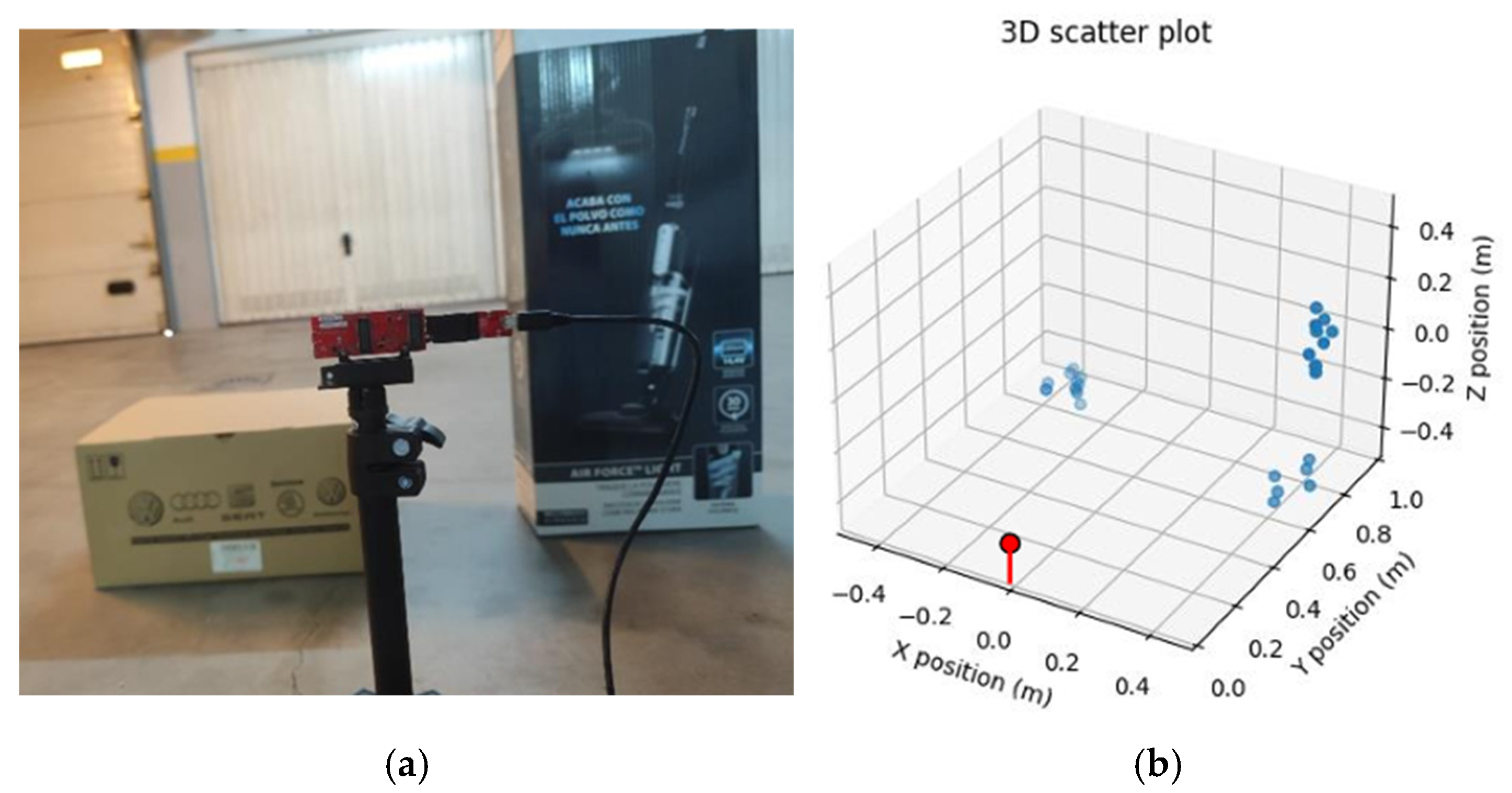
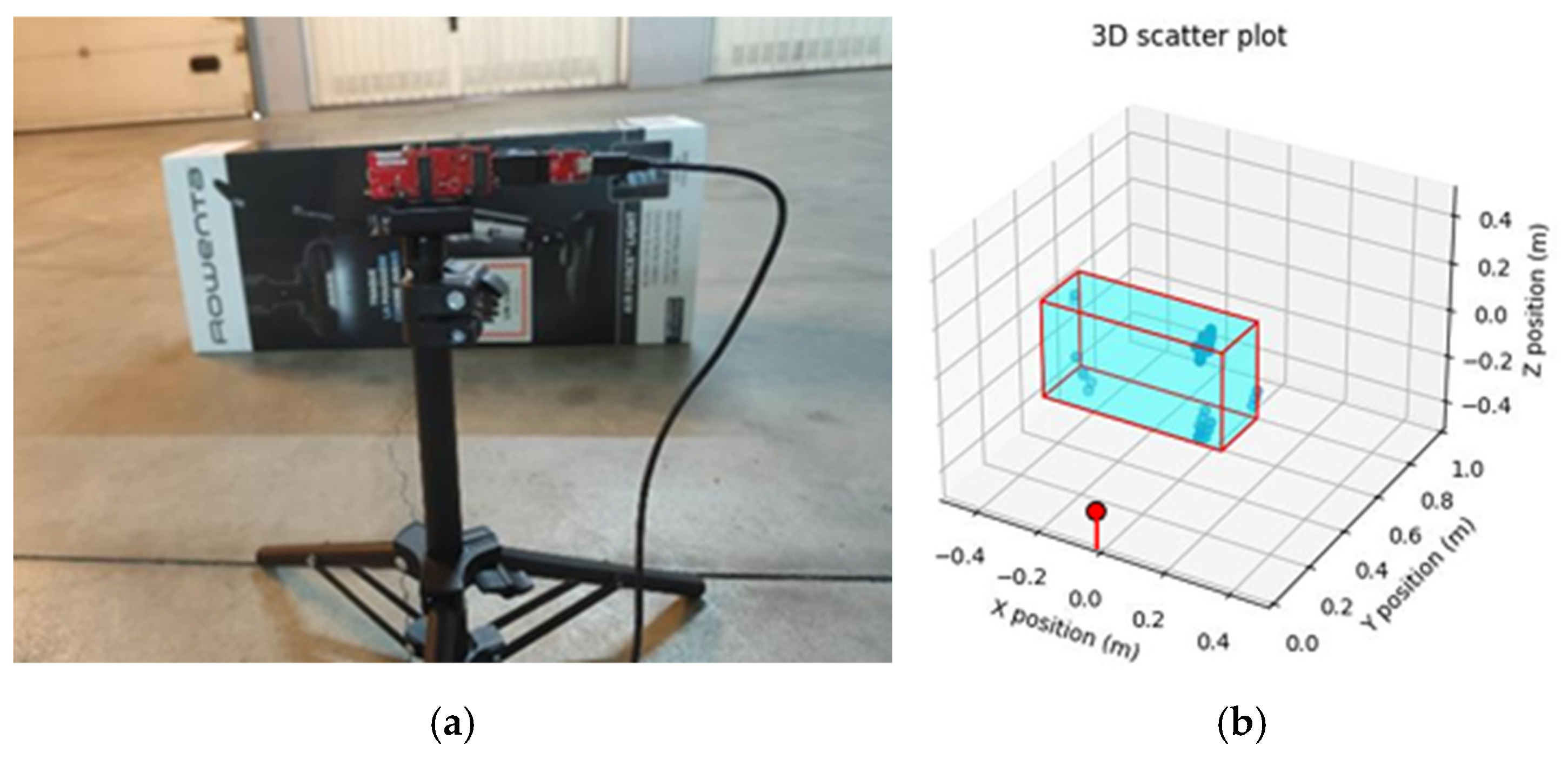
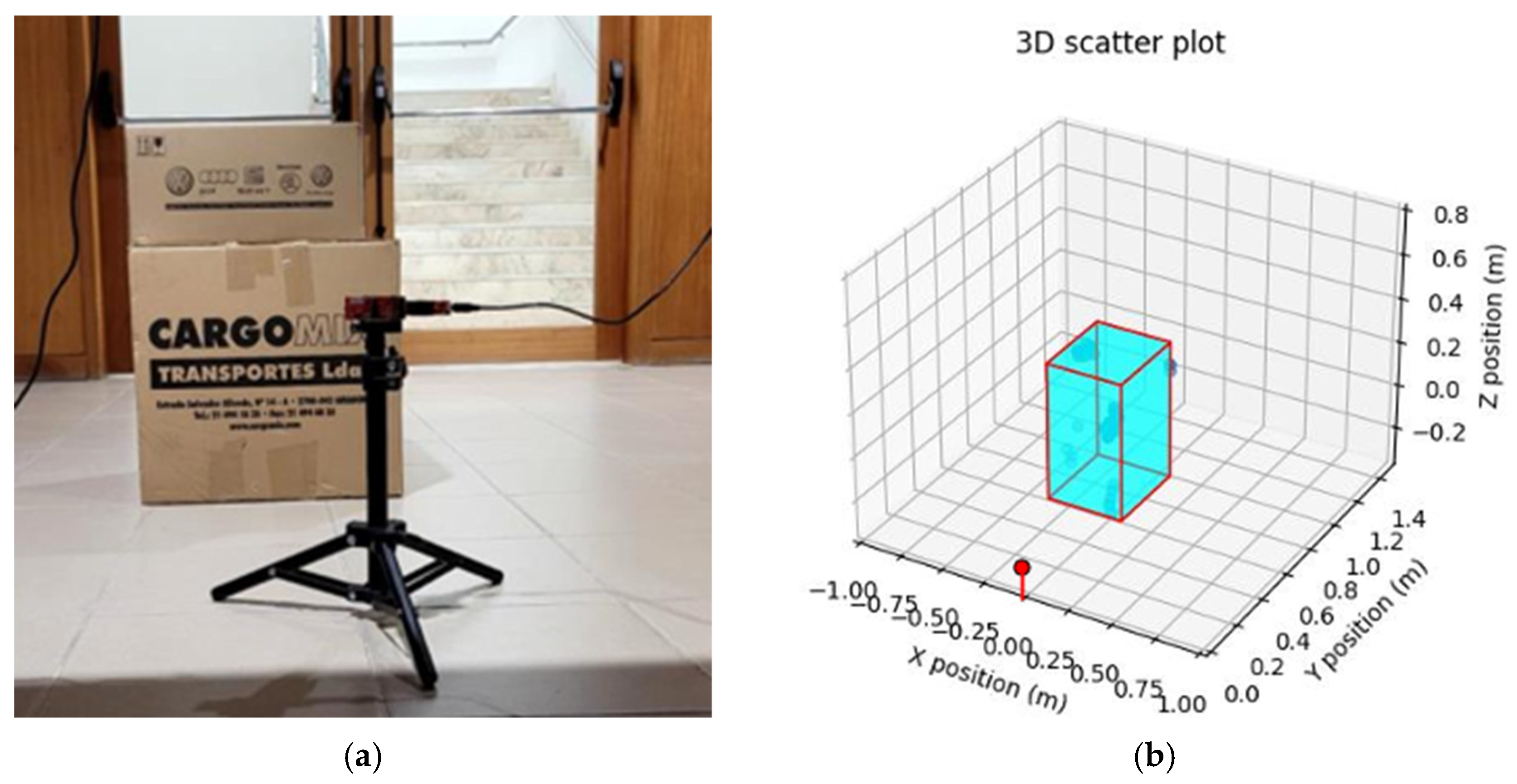
3.3. Laboratory Tests
- RF/Analog—This subsystem handles all radio frequency functions and analog signal processing. It is composed of the following:
- An oscillator that generates high-frequency signals used by the transmitters and receivers for modulation and demodulation of radar signals;
- Three transmitters, which include power amplifiers and modulation components;
- Four receivers, which include Low Noise Amplifiers (LNA), mixers, and filters;
- Filters and amplifiers improve the signal quality before conversion to a digital signal;
- ADCs to convert the received analog signals into digital signals for subsequent digital processing.
- Radio Processor—This subsystem is responsible for receiving and processing the signals from the previous subsystem. It is programmed by TI and consists of the following:
- A Digital Front-End typically serves as the interface between the analog unit and the digital processing modules. Its primary functions include gain control, sampling rate conversion, adaptive filtering, and phase correction [31].
- An ADC buffer is used to temporarily store the analog data before it is converted into digital format by the ADCs.
- A Ramp Generator—this component is essential in continuous wave frequency-modulated radar systems, such as this sensor. It generates the necessary frequency ramp to modulate the radar signals during transmission and reception, allowing for the measurement of distances and speeds of objects in the environment.
- A Radio (BIST) Processor for RF calibration and performing self-tests programmed by TI for self-diagnosis. It also includes RAM and FLASH memories.
- DSP Subsystem
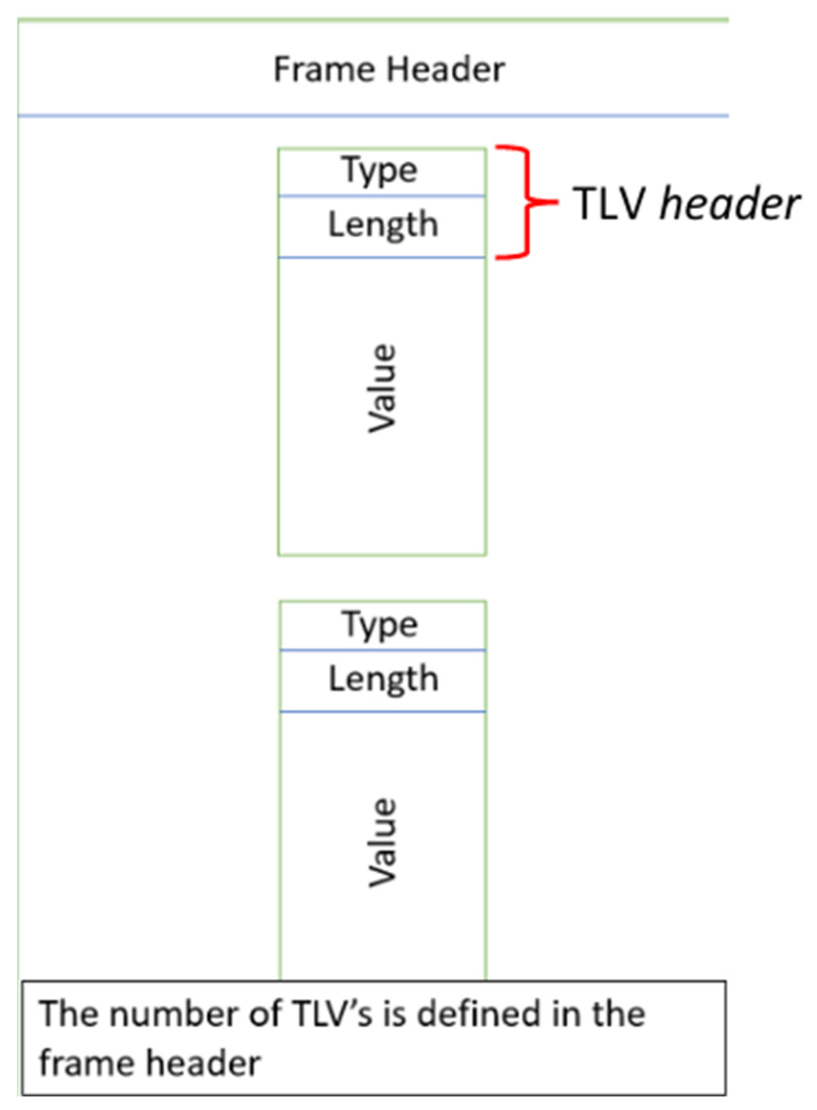
- 1—Detected Points, which contain the point cloud data. These data include the location (x, y, z) and the signal return intensity (Doppler), as we can see in Table 4.
- 2—Range Profile, which contains the range profile data, showing the intensity of the reflected signal as a function of distance.
- 3—Side Info for Detected Points, where the payload consists of 4 bytes for each detected object in the point cloud. This provides the Signal-to-Noise Ratio (SNR) and noise value for each object, as presented in Table 5. These values are measured in multiples of 0.1 dB.
4. Results
4.1. Initial Tests and Optimizations
- The third is an outlier that corresponds to the wall, for which the distance was also measured.
- Epsilon (ε)—which refers to the maximum distance between two points for them to be considered neighbors;
- MinPts—the minimum number of points within a radius of ε that defines a point with high density.
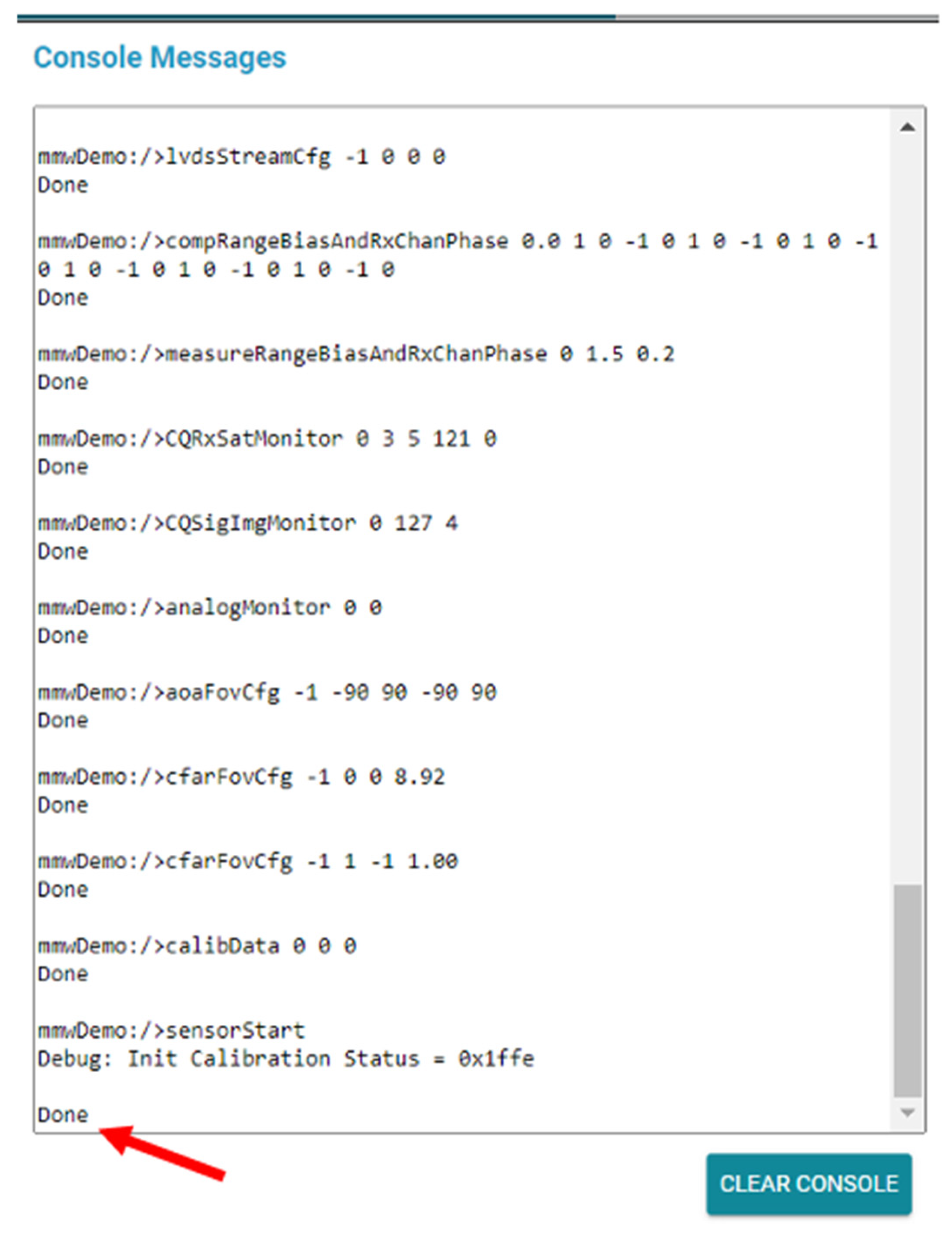
- aoaFovCfg—Command for the datapath to filter detected points outside the specified limits in the elevation plane or azimuth range. It consists of five parameters: subFrameIdx, minAzimuthDeg, maxAzimuthDeg, minElevationDeg, and maxElevationDeg. The minAzimuthDeg and maxAzimuthDeg parameters indicate the minimum and maximum azimuth angles, in degrees, specifying the start of the field of view, while the minElevationDeg and maxElevationDeg parameters indicate the minimum and maximum elevation angles, in degrees, specifying the start of the field of view. These parameters were changed from −90, 90, −90, 90 to −60, 60, −60, 60 to increase the precision in the area of focus by the radar sensor.
- cfarCfg—Command with the CFAR configuration message for the datapath, consisting of nine parameters: subFrameIdx, procDirection, mode, noiseWin, guardLen, divShift, cyclic/Wrapped mode, Threshold, and peak grouping. This command is introduced twice to define two processing directions. The processing directions are defined in the procDirection parameter, where the value 0 corresponds to CFAR detection in the range direction, and the value 1 corresponds to CFAR detection in the Doppler direction. The peak grouping parameter was changed from 1 to 0 in both commands to disable peak grouping. Additionally, the Threshold parameter was changed from 15 to 18 in the command where procDirection is 1, and in the command where procDirection is 0, the Threshold parameter was changed from 15 to 14.
- staticBoundaryBox—Defines the area where the load is expected to remain static for a long period. It consists of six parameters: X-min, X-max, Y-min, Y-max, Z-min, and Z-max. The X-min and X-max parameters were set to −1 and 1, defining the minimum and maximum horizontal distances from the origin. The Y-min and Y-max parameters were set to 0 and 1.5, defining the minimum and maximum vertical distances from the origin, and the Z-min and Z-max parameters were set to −0.35 and 1, defining the minimum and maximum height relative to the origin.
- sensorPosition—This is used to specify the orientation and position of the radar sensor and consists of three parameters: sensorHeight, azimTilt, and elevTilt. The sensorHeight parameter defines the height of the radar sensor above the ground plane, which was set to 0.34; the azimTilt parameter defines the azimuth tilt of the radar sensor, which was set to 0; and the elevTilt parameter defines the elevation tilt of the radar sensor, which was also set to 0.
- cfarFovCfg—Command for the datapath to filter detected points outside the specified limits in the range direction or Doppler direction. It consists of four parameters: subFrameIdx, procDirection, min, and max. This command is introduced twice to allow the definition of two processing directions. The processing directions are defined in the procDirection parameter, where 0 corresponds to filtering points in the range direction and 1 corresponds to filtering points in the Doppler direction. The min parameter corresponds to the minimum limit for range or Doppler, below which detected points are filtered, and the max parameter corresponds to the maximum limit for range or Doppler, above which detected points are filtered. In the command where procDirection is 0, the min and max parameters were set to 0 and 1.5, respectively. In the command where procDirection is 1, the min and max parameters were set to −1 and 1, respectively.
4.2. Final Results
- During the tests conducted, the values for the width, length, and height of the various objects showed some deviations from their actual size, but the other dimensions compensated for this deviation, making the calculated volume close to the real volume. This error does not significantly impact the project, as for the use case of this project, only the final volume presented is considered.
- Based on the results obtained, and if errors up to 10% are tolerable, it is concluded that this new solution has significant potential to enter the market and compete with other existing technologies.
- During the tests, only the packets with TLV type 1 were processed, as they contained all the necessary information for the focus of this project. That being said, and considering the structure of the datagram and the size of its fields, presented in Section 3.2 of this document, we can conclude that the size of the data being processed is, in bytes, , where these represent the size of the frame header, the size of the TLV header, the number of detected objects, and the size of the TLV type 1 payload.
- Throughout this work, it was not possible to mitigate some identified sources of error, such as the use of objects that were not in the best conditions for measurements. In particular, the presence of tape on the objects could interfere with the accuracy of the measurements due to its impact on light reflection. Additionally, the sensor’s placement could be optimized, as its current position did not always allow for an ideal view of the objects in some cases. Placing it in a higher position, allowing for observation of the objects from a superior angle, could help reduce incorrect measurements, especially in scenarios where there were boxes behind the visible ones. It was also observed that the test environment was not ideal, as the presence of additional objects and insufficient isolation could cause interference with the sensor, compromising the accuracy of the results.
- In this work, it was also observed that in the case of very small objects, the sensor’s accuracy was not optimal, at least with the sensor configuration we used throughout this project.
- The time between placing the objects in space and obtaining their measurement results is approximately 5 s.
- The effectiveness of the system was evaluated at various distances, and the experiments indicated that it becomes more reliable from 0.6 m onwards. Based on this observation, all tests were conducted starting from this distance. However, the determination of the minimum detectable object size was not specifically addressed in this study. This limitation could be explored in future work by analyzing the relationship between object dimensions and measurement accuracy under different experimental conditions.
5. Conclusions and Future Work
Author Contributions
Funding
Data Availability Statement
Acknowledgments
Conflicts of Interest
Appendix A


Appendix B
| Commands for sensor configuration |
| sensorStop flushcfg sensorPosition 0.34 0 0 dfeDataoutputMode 1 channelcfg 15 7 0 adcCfg 2 1 adcbufcfg -1 0 1 1 1 profilecfg 0 60 359 7 57.14 0 0 70 1 256 5209 0 0 158 chirpCfg 0 0 0 0 0 1 chirpCfg 1 1 0 0 0 2 chirpCfg 2 2 0 0 0 4 frameCfg 0 2 16 0 100 1 0 lowPower 0 0 guiMonitor -1 1 1 0 0 0 1 cfarCfg 1 0 2 8 4 3 0 14 0 cfarCfg -1 1 0 4 2 3 1 18 0 multiobjBeamForming -1 1 0.5 clutterRemoval -1 0 calibDcRangeSig -1 0 -5 8 256 extendedMaxVelocity -1 0 lvdsStreamCfg -1 0 0 0 compRangeBiasAndRxChanPhase 0.0 1 0 -1 0 1 0 -1 0 1 0 -1 0 1 0 -1 0 1 0 -1 0 measureRangeBiasAndRxChanPhase 0 1.5 0.2 CQRxSatMonitor 0 3 5 121 0 CQSigImgMonitor 0 127 4 analogMonitor 0 0 aoaFovCfg -1 -60 60 -60 60 cfarFovCfg -1 0 0 1.5 cfarFovCfg -1 1 -1 1.00 calibData 0 0 0 staticBoundaryBox -1 1 0 1.5 -0.35 1 sensorStart |
References
- The Internet of Cargo. The IoT Transformation Company. The Internet of Cargo. Available online: https://www.sensefinity.com/ (accessed on 9 July 2024).
- Introduction to IoT. Available online: https://www.researchgate.net/publication/330114646_Introduction_to_IOT (accessed on 6 March 2024).
- Teicher, J. The Little-Known Story of the First IOT Device, IBM Blog. 2019. Available online: https://www.ibm.com/blog/little-known-story-first-iot-device/ (accessed on 6 March 2024).
- Vailshery, L.S. IOT Connected Devices Worldwide 2019–2030, Statista. 2023. Available online: https://www.statista.com/statistics/1183457/iot-connected-devices-worldwide/ (accessed on 7 March 2024).
- What Is Iot? Internet of Things Explained—AWS. Available online: https://aws.amazon.com/what-is/iot/ (accessed on 6 March 2024).
- Iberdrola. O Que É a Iiot? Descubra a Internet Industrial das Coisas, Iberdrola. 2021. Available online: www.iberdrola.com/innovation/what-is-iiot (accessed on 6 March 2024).
- Industrial Internet of Things Market to Reach $1693.30bn by 2030 Industrial Internet of Things Market To Reach $1693.30Bn by 2030. Available online: https://www.grandviewresearch.com/press-release/global-industrial-internet-of-thingsiiot-market (accessed on 7 March 2024).
- Mecalux A Revolução da Internet Industrial das Coisas (IIoT), Mecalux, Soluções de Armazenagem. Available online: https://www.mecalux.pt/blog/iiot-internet-industrial-dascoisas (accessed on 7 March 2024).
- What Is Ultrasonic Sensor: Working Principle & Applications Robocraze. Available online: https://robocraze.com/blogs/post/what-is-ultrasonic-sensor (accessed on 15 October 2024).
- Infrared Sensor—IR Sensor: Sensor Division Knowledge Infrared Sensor—IR Sensor. Sensor Division Knowledge. Available online: http://www.infratec.eu/sensor-division/service-support/glossary/infrared-sensor/ (accessed on 20 March 2024).
- Devasia, A. Infrared Sensor: What Is It & How Does It Work, Safe and Sound Security. 2023. Available online: https://getsafeandsound.com/blog/infrared-sensor/ (accessed on 20 March 2024).
- Utama, H.; Kevin; Tanudjaja, H. Smart Street Lighting System with Data Monitoring. In Proceedings of the IOP Conference Series: Materials Science and Engineering, Chandigarh, India, 28–30 August 2020. Available online: https://iopscience.iop.org/article/10.1088/1757-899X/1007/1/012148 (accessed on 20 March 2024).
- Yokoishi, T.; Mitsugi, J.; Nakamura, O.; Murai, J. Room occupancy determination with particle filtering of networked pyroelectric infrared (PIR) sensor data. In Proceedings of the Sensors, 2012 IEEE, Taipei, Taiwan, 28–31 October 2012; pp. 1–4. [Google Scholar] [CrossRef]
- Laser Sensor Explained: Types and Working Principles—Realpars RSS. Available online: https://www.realpars.com/blog/laser-sensor (accessed on 22 March 2024).
- Laser Sensors Keyence. Available online: https://www.keyence.com/products/sensor/laser/ (accessed on 22 March 2024).
- Huang, X.; Tsoi, J.K.P.; Patel, N. mmWave Radar Sensors Fusion for Indoor Object Detection and Tracking. Electronics 2022, 11, 2209. [Google Scholar] [CrossRef]
- The Fundamentals of Millimeter Wave Radar Sensors (rev. A). Available online: https://www.ti.com/lit/spyy005 (accessed on 22 March 2024).
- Ti Developer Zone. Available online: https://dev.ti.com/tirex/explore/node?node=A__AXNV8Pc8F7j2TwsB7QnTDw__RADAR-ACADEMY__GwxShWe__LATEST (accessed on 27 March 2024).
- Soumya, A.; Krishna Mohan, C.; Cenkeramaddi, L.R. Recent Advances in mmWave Radar-Based Sensing, Its Applications, and Machine Learning Techniques: A Review. Sensors 2023, 23, 8901. [Google Scholar] [CrossRef] [PubMed]
- Shastri, S.; Arjoune, Y.; Amraoui, A.; Abou Abdallah, N.; Pathak, P.H. A Review of Millimeter Wave Device-Based Localization and Device-Free Sensing Technologies and Applications. IEEE Commun. Surv. Tutor. 2022, 24, 1708–1749. [Google Scholar] [CrossRef]
- Wang, Z.; Dong, Z.; Li, J.; Zhang, Q.; Wang, W.; Guo, Y. Human activity recognition based on millimeter-wave radar. In Proceedings of the 2023 5th International Conference on Frontiers Technology of Information and Computer (ICFTIC), Qiangdao, China, 17–19 November 2023; pp. 360–363. [Google Scholar] [CrossRef]
- Amar, R.; Alaee-Kerahroodi, M.; Mysore, B.S. FMCW-FMCW Interference Analysis in mm-Wave Radars; An indoor case study and validation by measurements. In Proceedings of the 2021 21st International Radar Symposium (IRS), Berlin, Germany, 21–22 June 2021; pp. 1–11. [Google Scholar] [CrossRef]
- Pearce, A.; Zhang, J.A.; Xu, R.; Wu, K. Multi-Object Tracking with mmWave Radar: A Review. Electronics 2023, 12, 308. [Google Scholar] [CrossRef]
- Devnath, M.K.; Chakma, A.; Anwar, M.S.; Dey, E.; Hasan, Z.; Conn, M.; Pal, B.; Roy, N. A Systematic Study on Object Recognition Using Millimeter-wave Radar. In Proceedings of the 2023 IEEE International Conference on Smart Computing (SMARTCOMP), Nashville, TN, USA, 26–30 June 2023; pp. 57–64. [Google Scholar] [CrossRef]
- Sonny, A.; Kumar, A.; Cenkeramaddi, L.R. Carry Object Detection Utilizing mmWave Radar Sensors and Ensemble-Based Extra Tree Classifiers on the Edge Computing Systems. IEEE Sens. J. 2023, 23, 20137–20149. [Google Scholar] [CrossRef]
- TI. Available online: https://www.ti.com/lit/ds/symlink/iwr6843aop.pdf?ts=1617800733758&ref_url=https%2 53A%252F%252Fwww.ti.com%252Fproduct%252FIWR6843AOP (accessed on 5 April 2024).
- Ti Developer Zone. Available online: https://dev.ti.com/tirex/explore/node?devtools=AWR6843AOPEVM&node=A__AGnx4WbbqMvEcH9P.cgwvg__com.ti.mmwave_devtools__FUz-xrs__LATEST (accessed on 6 April 2024).
- IWR6843AOPEVM Evaluation Board. TI.com. Available online: https://www.ti.com/tool/IWR6843AOPEVM (accessed on 7 April 2024).
- Chakraborty, S.; Nagwani, N.K. Performance Comparison of Incremental K-Means and Incremental DBSCAN Algorithms. Int. J. Comput. Appl. 2011, 27, 11–16. [Google Scholar] [CrossRef]
- TI. Available online: https://www.ti.com/product/IWR6843AOP (accessed on 5 April 2024).
- Digital Front—An Overview. ScienceDirect Topics. Available online: https://www.sciencedirect.com/topics/engineering/digital-front (accessed on 20 May 2024).
- Best Practices for Placement and Angle of mmwave Radar. Available online: https://www.ti.com/lit/pdf/swra758 (accessed on 10 July 2024).
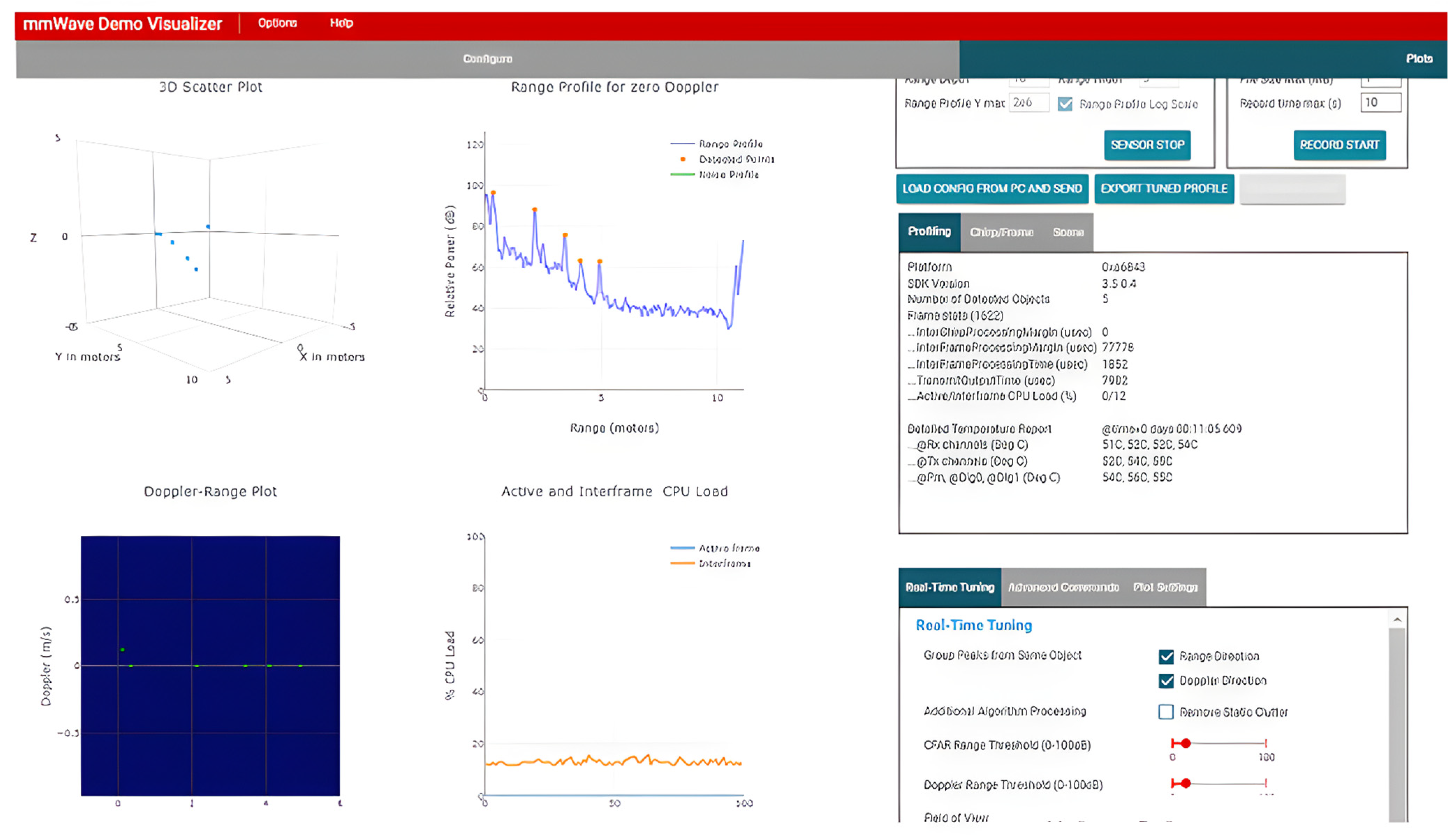
- MmWave Demo Visualizer. Available online: https://dev.ti.com/gallery/view/mmwave/mmWave_Demo_Visualizer/ver/3.5.0/ (accessed on 5 April 2024).
- Ti Developer Zone. Available online: https://dev.ti.com/tirex/explore/node?a=1AslXXD__1.00.01.07&node=A__ADnbI7zK9b SRgZqeAxprvQ__radar_toolbox__1AslXXD__1.00.01.07 (accessed on 5 April 2024).
- Mmwave SDK User Guide Scribd. Available online: https://www.scribd.com/document/653462094/mmwave-sdk-user-guide (accessed on 5 April 2024).
- Paramita, A.S.; Hariguna, T. Comparison of K-Means and DBSCAN Algorithms for Customer Segmentation in E-commerce. J. Digit. Mark. Digit. Curr. 2024, 1, 43–62. [Google Scholar] [CrossRef]


| Value | Type | Bytes | Details |
|---|---|---|---|
| Magic word | uint16_t | 8 | Output buffer magic word (sync word), it is initialized to, e.g., 0x0102 |
| Version | uint32_t | 4 | SDK Version |
| Total Packet Length | uint32_t | 4 | Total packet length including frame header |
| Platform | uint32_t | 4 | Device type, e.g., 0xA6843 |
| Frame Number | uint32_t | 4 | Frame number |
| Time [in CPU cycles] | uint32_t | 4 | Time in CPU cycles when the message was created |
| Num Detected Obj | uint32_t | 4 | Number of detected objects (points) for the frame |
| Num TLVs | uint32_t | 4 | Number of TLV items for the frame |
| Subframe Number | uint32_t | 4 | 0 if advanced subframe mode not enabled, otherwise range 1 to number of frame-1 |
| Value | Type | Bytes | Details |
|---|---|---|---|
| Type | uint32_t | 4 | Indicates types of the message contained in the payload |
| Length | uint32_t | 4 | Length of the payload in bytes (not including TLV header) |
| Type Identifier | Value Type |
|---|---|
| 1 | Detected Points |
| 2 | Range Profile |
| 3 | Noise Floor Profile |
| 4 | Azimuth Static Heatmap |
| 5 | Range-Doppler Heatmap |
| 6 | Statistics (Performance) |
| 7 | Side Info for Detected Points |
| 8 | Azimuth/Elevation Static Heatmap |
| 9 | Temperature Statistics |
| Value | Type | Bytes |
|---|---|---|
| X [m] | float | 4 |
| Y [m] | float | 4 |
| Z [m] | float | 4 |
| Doppler [m/s] | float | 4 |
| Value | Type | Bytes |
|---|---|---|
| SNR [dB] | uint16_t | 2 |
| Doppler [m/s] | uint16_t | 2 |
| Parameter | Old Value | Optimized Value | Description |
|---|---|---|---|
| aoaFovCfg | −90, 90, −90, 90 | −60, 60, −60, 60 | Restricts the radar field of view to increase precision |
| cfarCfg (procDirection = 1) | Threshold = 15 | Threshold = 18 | Adjusts CFAR threshold for Doppler detection |
| cfarCfg (procDirection = 0) | Threshold = 15, Peak grouping = 1 | Threshold = 14, Peak grouping = 0 | Adjusts CFAR threshold for range detection and disables peak grouping |
| staticBoundaryBox | We added this parameter to configuration file | X-min = −1 X-max = 1, Y-min = 0, Y-max = 1.5, Z-min = −0.35, Z-max = 1 | Defines a specific area where the load is expected to remain static |
| sensorPosition | We added this parameter to configuration file | Height = 0.34, AzimTilt = 0, ElevTilt = 0 | Specifies radar sensor placement |
| cfarFovCfg (procDirection = 1) | No changes needed | Filter detected points outside the specified limits in the range direction or Doppler direction. | |
| cfarFovCfg (procDirection = 0) | max = 8.92 | max = 1.5 | |
| Experiment | X Measured (m) | X Actual (m) | X Error (%) | Y Measured (m) | Y Actual (m) | Y Error (%) | Z Measured (m) | Z Actual (m) | Z Error (%) |
|---|---|---|---|---|---|---|---|---|---|
| 1 | 0.5717 | 0.45 | 27 | 0.297 | 0.35 | 15 | 0.435 | 0.44 | 1.13 |
| 2 | 0.853 | 0.905 | 5.75 | 0.391 | 0.35 | 11.7 | 0.4 | 0.435 | 8 |
| 3 | 0.444 | 0.45 | 1.33 | 0.385 | 0.355 | 8.45 | 0.6282 | 0.625 | 0.51 |
| 4 | 0.7467 | 0.62 | 20.44 | 0.2877 | 0.35 | 17.8 | 0.58324 | 0.55 | 6.04 |
| 5 | 0.56552 | 0.62 | 8.787 | 0.3867 | 0.35 | 10.48 | 0.6214 | 0.63 | 1.365 |
| Experiment | X Range (m) | Y Range (m) | Z Range (m) | Sensor Volume () | Actual Volume () | Error (%) |
|---|---|---|---|---|---|---|
| 1 | Min: −0.1717 Max: 0.4 | Min: 0.5979 Max: 0.89538 | Min: −0.349 Max: 0.08585 | 0.074 | 0.0693 | 6.78 |
| 2 | Min: −0.78355 Max: 0.0695 | Min: 0.61 Max: 1 | Min: −0.324 Max: 0.0736 | 0.1331 | 0.1378 | 3.53 |
| 3 | Min: −0.38155 Max: 0.0627 | Min: 0.61 Max: 0.993 | Min: −0.37065 Max: 0.2575 | 0.1074 | 0.0998 | 7.61 |
| 4 | Min: −0.5178 Max: 0.22893 | Min: 0.5943 Max: 0.882 | Min: −0.2725 Max: 0.3107 | 0.1253 | 0.1194 | 4.94 |
| 5 | Min: −0.34476 Max: 0.22076 | Min: 0.5655 Max: 0.9522 | Min:−0.2453 Max: 0.3761 | 0.1359 | 0.1367 | 0.6 |
Disclaimer/Publisher’s Note: The statements, opinions and data contained in all publications are solely those of the individual author(s) and contributor(s) and not of MDPI and/or the editor(s). MDPI and/or the editor(s) disclaim responsibility for any injury to people or property resulting from any ideas, methods, instructions or products referred to in the content. |
© 2025 by the authors. Licensee MDPI, Basel, Switzerland. This article is an open access article distributed under the terms and conditions of the Creative Commons Attribution (CC BY) license (https://creativecommons.org/licenses/by/4.0/).
Share and Cite
Pires, L.M.; Alves, T.; Vassaramo, M.; Fialho, V. Design and Development of a High-Accuracy IoT System for Real-Time Load and Space Monitoring in Shipping Containers. Designs 2025, 9, 43. https://doi.org/10.3390/designs9020043
Pires LM, Alves T, Vassaramo M, Fialho V. Design and Development of a High-Accuracy IoT System for Real-Time Load and Space Monitoring in Shipping Containers. Designs. 2025; 9(2):43. https://doi.org/10.3390/designs9020043
Chicago/Turabian StylePires, Luis Miguel, Tiago Alves, Mikil Vassaramo, and Vitor Fialho. 2025. "Design and Development of a High-Accuracy IoT System for Real-Time Load and Space Monitoring in Shipping Containers" Designs 9, no. 2: 43. https://doi.org/10.3390/designs9020043
APA StylePires, L. M., Alves, T., Vassaramo, M., & Fialho, V. (2025). Design and Development of a High-Accuracy IoT System for Real-Time Load and Space Monitoring in Shipping Containers. Designs, 9(2), 43. https://doi.org/10.3390/designs9020043