Abstract
Topology optimization is increasingly employed to design fluid flow systems capable of achieving optimal performance under specific constraints. This study presents a density-based topology optimization approach specifically tailored for second-order reactive flows. The fluid-solid distribution within the domain is represented by continuous design variables expressed as an inverse permeability field. An adjoint method is used to efficiently compute gradients of the objective function, enabling the application of gradient-based algorithms to solve the optimization problem. The methodology is validated on a benchmark bend-pipe case, reproducing known optimal geometry. Subsequently, the method is applied to optimize a system involving second-order chemical reactions, aiming to maximize a desired reaction while limiting undesirable side reactions. Results demonstrate significant performance improvements, achieving gains in reaction efficiency ranging from 90.4% to 98.7% for the porous geometries and from 94.6% to 105.2% for real geometries. The optimization strategy successfully generates flow configurations analogous to those observed in modern gas turbines, highlighting the practical relevance and potential impact of the developed methodology.
1. Introduction
Despite increasingly stringent environmental standards, the combustion engine remains a relevant solution due to its ease of design and use, as well as its performance and energy density when renewable low-carbon fuels are envisioned. Two of the main challenges in the design of combustion engines are their energy efficiency and their ability to generate low levels of nitrogen oxides, abbreviated as NOx. The predominant mechanism in the formation of NOx is the Zeldovich mechanism. It describes how nitrogen monoxide, called thermal NO, is formed in high-temperature zones. To limit the formation of thermal NO, the most common strategy is to dilute the combustion with a secondary flow to lower the temperature and thus limit the mechanism [1,2,3]. This strategy involves adopting specific geometries that can lower other objectives, for example, decreasing combustion efficiency or increasing pressure losses. The complexity of the problem therefore makes the design of combustion chambers a difficult task that is still carried out empirically today. However, numerical simulations have in recent years accelerated the process by allowing us to study the shape evolution impact on flows, stresses and systems without practical experiments. Nevertheless, in many cases the change or evolution of geometries still relies on know-how and experience, sometimes intuition or simply accident. The quest for better flows, structures or systems calls for optimal design, a methodology that provides the best shape able to fulfill a goal given some constraints. In that way, a direct solution for the best geometry could be obtained without repetition of modification and testing, whether in simulation or experiments. In fluid dynamics, since flow is imposed by geometry, it is legitimate to question the optimal geometry of a system to achieve a given objective. Topology optimization (TO) methods introduced by Borrvall and Petersson [4] in fluid dynamics allow addressing this issue. Since their introduction, these methods have been used in various applications; Alexandersen and Andreasen provide a review on the subject [5], along with Li et al. [6]. The fields where topological optimization applies are widening, particularly in fluids [7,8,9]. In the case of reactive flows, Okkels and Bruus [10,11] propose applying the density method to maximize the average reaction rate of chemical species involved in catalytic microreactors. To do this, they use first-order chemical reactions coupled with chemical species transport equations and the Navier–Stokes equations, solving the optimization problem using the MMA method (Method of Moving Asymptotes). Schäpper et al. [12] have proposed to use the method to optimize biomass distribution in a bioreactor. Yaji et al. [13] also use the density method to optimize the flow geometry in a redox battery and use the SLP (Sequential Linear Programming) method to solve the optimization problem. Behrou et al. [14] use the density method to optimize the flow of proton exchange membrane fuel cells and solve a multi-objective optimization problem with the GCMMA method (Globally Convergent Method of Moving Asymptotes). Dugast et al. [15] propose maximizing the reaction rate of a flow in the presence of a catalyst, using the lattice Boltzmann method coupled with a level-set method, and show the method’s efficiency and robustness for different Damkohler and Péclet numbers. Liu et al. [16] base their work on Okkels and Bruus to study the impact of different parameters on the performance of an optimized catalytic microreactor. Jia et al. [17] use a multi-objective TO method to improve a solar reactor for the first-order reaction of methane decomposition. The cost functions are the heat exchange capability and the viscous dissipation. The reaction rate is improved only through an increase in temperature. Bhattacharjee and Atta [18] use TO in order to increase the reaction rate of a non-Newtonian fluid in a catalytic microreactor with the density method and the MMA resolution algorithm. Wang et al. [19] also have optimized a catalytic microreactor with the density method but propose a multi-objective cost function that considers flow dissipation energy, pressure losses, and reaction rate. Finally, Gua et al. [20] use TO to optimize microreactors for hydrogen production with a first-order catalytic reaction, and the objective functions are only power dissipation and average temperature. Since the introduction of TO for reactive flows, only a few articles have addressed the subject, and previous works from different authors have only addressed first-order catalytic reactions, whereas many real-life systems work on second-order chemical reactions like combustion processes. Urgent research is needed on multi-objective topology optimization for second-order chemical reactions in flow, particularly in practical applications such as combustion.
In the following we will address the novel geometry optimization for flow with two second-order chemical reactions. The objective is to maximize a first exothermic second-order chemical reaction, like combustion, while constraining another second-order chemical reaction, like the Zeldovich mechanism. The presented algorithm also considers the constraints of dissipated power that can be encountered during the design process of a combustion chamber. The developed methodology is first presented and justified among different alternatives. To validate the algorithm, the well-known case of minimizing dissipated power in a bend pipe was performed, and the results are compared to the literature. Another illustration of the method effectiveness is made through the minimization of dissipation through a pipe, leading to the well-known cone shape. After validation, a simple case with six different constraint values for the second chemical reaction was conducted, and the results were analyzed. It should be noted that the purpose is to develop an optimization methodology, meaning that CFD simulations are not the core of the study but a tool, assumed to be functional, to deliver flow features. Convergence and precision of the CFD simulations have been widely explored in the literature and are not discussed in the following, which focuses on the optimization methodology with given CFD simulation parameters. To guarantee a precise solution of flows, CFD simulations are carried out at low Reynolds numbers. Optimization of geometries for flows at any Reynolds number is possible once the optimization method is operational, at the cost of higher calculation time.
2. Topology Optimization of Flow
Topology optimization involves finding the optimal layout of a structure subject to constraints within a given region, with the physical size and shape of the structure initially unknown. In other words, assuming that the geometry is described by parameters , called “design variables,” and that they constitute the “design vector,” , , topology optimization involves determining the vector that minimizes or maximizes a “cost” function within a given volume , subject to a “constraint vector” of dimension . Design variables ideally take two values:
The discrete nature of these variables presents hard challenges [21], so it is preferable to use continuous design variables, , with the objective of making this variable tend locally towards 0 or 1.
2.1. Geometry Description
In the case of a physical problem, to determine the optimal topology of a system, it is necessary to define the design variables and give them a physical interpretation to mathematically describe the system’s geometry. According to the state of the art by Alexandersen and Andreasen [2], in fluid dynamics, the “level set” and “density” methods are predominant, with a clear advantage for the latter. The density method belongs to a family of methods called “material interpolation,” which use the physical properties of the material as design variables [22]. This family was initiated by Bendsøe [14] with the “homogenization approach” method, followed shortly after by the SIMP (Simplified Isotropic Material with Penalization) density method developed by Bendsøe, Zhou, Rozvany, Mlejnek [23,24,25], which was introduced to simplify the homogenization method and improve convergence towards the optimal geometry [26]. Borrvall and Petersson introduced this method in fluid dynamics by considering a porous medium; the flow geometry is thus directly translated by the inverse permeability field. This field is discretized with a mesh often identical to the pressure and velocity fields. A mesh with zero inverse permeability indicates that the area is fluid, and a mesh with infinite inverse permeability indicates that the area is solid. An additional term is added to the momentum conservation equation to translate the effect of porosity on the flow:
where is the inverse permeability field. Borrvall and Petersson proposed the following convex interpolation function, which gives the relationship between the design vector and the inverse permeability [1]:
and are the maximum and minimum values of the field , respectively. The penalization parameter allows controlling the gray regions (intermediate regions between solid and fluid); the larger the , the more discrete the obtained geometry will be, but also will the higher the risk of obtaining a local optimum. To obtain a discrete geometry while avoiding local optima, Borrvall and Petersson propose a two-step procedure: a first resolution with a relatively low penalization parameter , then a second resolution with the geometry obtained in the first step as the initial geometry and a higher penalization number . This allows the second step to have a better-conditioned optimization problem and thus avoid local optima. The Darcy number for the local flow is defined as is set at , where is the characteristic velocity and is the characteristic length.
2.2. Optimum Search Algorithm
As seen previously, solving a topology optimization problem involves finding a set of design variables that minimizes or maximizes a cost function subject to constraints. There are two main families of optimum search methods: non-gradient and gradient methods.
2.2.1. Non-Gradient Methods
The first approach to finding the optimum is the stochastic and/or meta-heuristic approach, which imitates biological, physical, or other phenomena to converge towards the optimum, such as Particle Swarms [27,28,29], Simulated Annealing [30,31,32], Ant Colonies [33,34], Harmony search [35,36], Differential Evolution [37,38,39], Artificial Immune [40], Evolutionary Structural Optimization (ESO) [41,42], or the most popular among them, Genetic Algorithms [43,44]. The latter was introduced by Holland in 1975 [45] and falls into a broader category called Evolutionary algorithms [46]. To converge towards the global optimum, the initial population must cover the entire definition domain of the cost function. However, in topology optimization, the number of possible geometry combinations and, in some cases, the computation time required to solve the physical problem do not allow these algorithms to explore the entire study domain in reasonable computational times. Consequently, in some domains, these algorithms do not necessarily converge towards the global optimum [47]. However, there are cases where using non-gradient methods is more appropriate than gradient methods, particularly when it is impossible to describe the medium with a continuous variable or when it is impossible to regularize or convexify the problem [47].
2.2.2. Gradient Methods
To determine the optimum of a cost function, the second approach involves using the gradient information of this function. The descent method is an iterative method that can use this information to converge towards the optimum [48]. Consider a cost function , being the design vector at iteration ; the objective is to find at the next iteration the vector such that ; for this, the descent method uses the following relationship:
With a coefficient called “descent step” and the “descent direction” at iteration . In the case of gradient methods, the direction is calculated using the gradient of the cost function; this method seems to have been proposed for the first time by Cauchy in 1847 [49]. The gradient of the cost function consists of the derivatives of the cost function with respect to the components of the design vector , so the gradient has the same dimension as the design vector:
is the nabla/gradient operator and the dimension of the vector . The gradient method therefore assumes
There are other methods for calculating the direction, such as the conjugate gradient direction, which uses information from previous iterations; the Newton direction, which uses the Hessian matrix of the cost function; or the quasi-Newton direction, which uses an approximation of the Hessian matrix [48]. Furthermore, topology optimization problems are specific optimization problems since they are generally non-linear, subject to inequality or equality constraints, and rarely convex. To solve this type of problem without converging towards a local optimum, there are dedicated gradient algorithms, such as Sequential Quadratic Programming (SQP), Convex Linearization (CONLIN) [50], Method of Moving Asymptotes (MMA) [51] and Globally Convergent Method of Moving Asymptotes (GCMMA) [52]. According to Sigmund and Maute, the most widespread methods in topology optimization are the MMA and GCMMA methods [26].
2.2.3. Gradient Calculation
In the case where a gradient method is used to search for the optimum, one must calculate the gradient of the cost function. However, in topology optimization, this calculation is not immediate, and using the finite difference method is not appropriate since, for a system with design variables, it would be necessary to solve the system of equations times to calculate each derivative of the gradient. The “adjoint method” described hereafter allows that calculation while considerably limiting the computation time. In some physical problems, the design variable does not directly influence the cost function but influences certain physical properties , which in turn influence the cost function. For example, in fluid dynamics, the design variable acts on the pressure and velocity fields of the flow, and these fields act on the cost function. In fluid dynamics, it reduces to . Consider a cost function subject to a constraint vector of dimension such that , being the design vector of dimension . The derivative of the cost function with respect to the design variables is
Notice that to calculate this derivative, the sensitivities must be determined, but in most cases does not depend explicitly on , so these sensitivities are difficult to determine analytically. To avoid this calculation, one can introduce the Lagrangian of the problem [53,54]:
With the vector of Lagrange multipliers of dimension equal to that of and «. » a suitable scalar product. The derivative of the Lagrangian with respect to the design variables is
Or in a more appropriate form
The difficulty in calculating the derivative of the Lagrangian also lies in calculating the sensitivity , but the problem is bypassed by seeking as a solution to the adjoint state equation:
Finally, using the definition of the function , one can write
To determine the derivative of the cost function, the Lagrange multipliers must therefore be determined, first, by solving the “adjoint system” , then using the equation that gives the relationship between the derivative of the cost function and the partial derivative of the Lagrangian .
3. Case Study
3.1. Algorithm Validation with Bend Pipe Case and Duct Case
The main difficulty for optimization with the technique employed is calculating the gradient of the cost function. The adjoint method overcomes this difficulty, but the complexity of the equations and their resolution can lead to errors. To validate the gradient calculation, the method that seems the simplest but most time-consuming is to use the finite difference method to calculate the gradient and then compare the values with those obtained by the adjoint state method. To reduce computation time, it is possible to calculate only a few components of the gradient, as performed by Yoon [55]. However, to properly validate the gradient calculation, the sampling size must be significant, and the finite difference method inevitably leads to high computation time. The validation procedure used in this article therefore does not allow validating the gradient of the cost function but still allows validating the overall architecture of the algorithm. The validation of the architecture of the algorithm is assumed to be independent of the case studied. To validate the algorithm, the problem of minimizing the dissipated power of a flow given an inlet and an outlet and a square domain for possible geometry is solved, a problem widely studied in scientific literature. It is assumed that the studied flows are steady and laminar with constant density. With the use of the density method, the mass and momentum conservation equations are, respectively,
The optimization problem is
where is the mesh index, the number of cells, and the cell volume and the upper limit of volume are and , respectively. The gradients of the cost function are calculated with equation (Equation (12)), please see Appendix A.1 for more details. To determine the vector of Lagrange multipliers, the adjoint system must be solved Equation (11), details are provided in Appendix A.2. The resolution of the primal system and the adjoint systems was performed with the open-source code “OpenFOAM”, with an Intel Xeon Silver 4208 CPU using only one core. The solver employs the SIMPLE algorithm for solving both the primal and adjoint systems. For the calculation of the primal and adjoint systems, the stopping criteria is a residual of less than , with a maximum of iterations. It is assumed from experience in similar calculations that despite a residual greater than , 2000 iterations are sufficient to achieve good convergence. The search for the optimal design vector will be carried out with the help of the MMA algorithm. The study domain is two-dimensional and has the same dimension as the geometry used by Borrvall and Petersson [4]. The domain consists of quadrilateral blocks with sides measuring 10 mm. The fields and will be discretized into meshes identical to those of the pressure and velocity fields. To confirm mesh independence, the problem was also solved on a finer mesh. The Reynolds number is set at 100 and the upper limit of volume at 0.25. The penalization parameter was kept constant at a value of . The final objective value obtained is 0.3896; the gap with the value obtained by Yoon at the same Reynolds number [56] is approximately 0.5%. As shown in Figure 1, at these Reynolds numbers, the design obtained is a straight-line channel with rounded corners. This resulting geometry closely resembles that obtained by Borrvall and Petersson [4] and by Yoon [56].
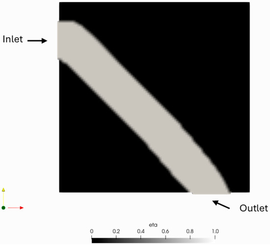
Figure 1.
Final geometry for the problem of minimizing dissipated power in bend pipe case.
In order to illustrate the method, a minimization of the dissipated power of laminar flow in the case of a duct is shown. The study domain consists of quadrilateral blocks with sides measuring 1 mm, as shown in Figure 2. The design area, where the geometry is modified, is indicated by the red rectangle in Figure 2.
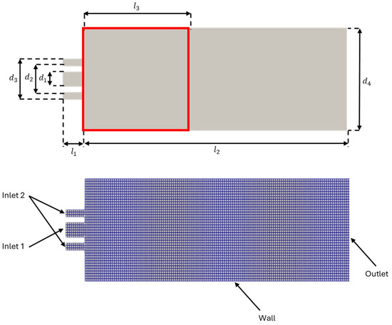
Figure 2.
Geometry and meshing of duct case.
The dimensions of the study domain are summarized in Table 1. The mesh is composed of hexahedrons with each side measuring 1 mm. The Reynolds number is set at 100. The penalization parameter was kept constant at a value of . The resulting geometry is presented in Figure 3, solid zones are colored in black. The geometry obtained to minimize the dissipated power is a well-known divergent cone.

Table 1.
Dimensions of the duct case domain.
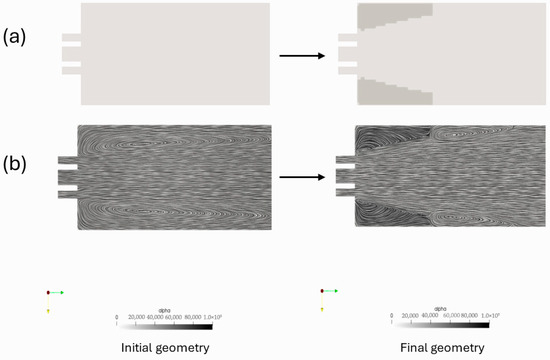
Figure 3.
(a) Initial and final geometries; (b) streamlines for the problem of minimizing dissipated power in duct case.
3.2. Optimization of Second-Order Chemical Reactions for 2D Duct Case
The assumption is made that the studied flows are steady and laminar with constant density. With the use of the density method, the mass and momentum conservation equations are, respectively,
Let us consider the following two second-order chemical reactions:
The rate constants and are calculated with the Arrhenius equation:
With T being temperature, A the pre-exponential factor, the activation energy and the universal gas constant. The transport equations for the mass fractions are as follows:
With being the molecular diffusivity. If one assumes that the first reaction is exothermic, and the enthalpy of reaction is denoted by , the energy equation transport is
The objective is to maximize the first chemical reaction (Equation (15)) and limit the second reaction (Equation (16)). In other words, the objective is to maximize the flow rate of the chemical species while limiting the flow rate of the chemical species . Thus, the optimization problem is
where and are the limits for and . The gradients of the cost function and the constraints and are calculated with Equation (Equation (12)); see Appendix A.1 for more details. To determine the vector of Lagrange multipliers, the adjoint system must be solved Equation (11), see Appendix A.2 for more details. The resolution of the primal system and the adjoint systems was performed with the open-source code “OpenFOAM”, with an Intel Xeon Silver 4208 CPU using only one core. The solver employs the SIMPLE algorithm [57] for solving both the primal and adjoint systems. For the calculation of the primal and adjoint systems, the stopping criteria is a residual of less than , with a maximum of iterations. Here again, it is assumed that despite a residual greater than , 2000 iterations are sufficient to achieve good convergence. The search for the optimal design vector will be carried out with the help of the MMA algorithm. The fields and will be discretized into meshes identical to those of the pressure and velocity fields. The study domain is identical to the domain presented in Figure 2 and Table 1. The Damköhler numbers, defined here as and , are set to 120. If the Damköhler numbers are too large, the geometry will have little influence on the reaction. To limit the stiffness of the equation system, the pre-exponential factors and are limited to 100, so to respect the Damköhler number, the inlet velocity is set to 0.167. The Reynolds numbers, defined as and are set at 1 to respect the laminar flow hypothesis. The cinematic viscosity is set to to respect the Reynolds number. The Schmidt number, defined as , is set to ; this number is taken high to favor the influence of the flow on the mixing. The Darcy number, defined as is set to to ensure strong damping of the flow in solid regions. At the inlet, the mass fraction of is set to 1 to simulate a fuel injection, and the mass fractions of the and species are, respectively, set to 0.2 and 0.8 to simulate the same composition of and as in air. The specific heat capacity is set to 1000, like air specific heat capacity. The enthalpy of reaction is set to , comparable to the enthalpy of reaction in combustion processes. The physical parameters and boundary conditions are, respectively, summarized in Table 2 and Table 3. The penalization parameter is equal to 0.01 for the first 500 iterations, then increases to 1 for the next 100 iterations, and finally to 10 for the last 100 iterations.
Table 2.
Physical parameters.
Table 3.
Boundary conditions of the primary system.
The optimization is performed with six constraint limits listed in Table 4. For the six constraint limits, the evolution of the cost function and constraint is presented in Figure 4. The results show that the algorithm maximizes the cost function and reaches a geometry that respects the constraints for all performed constraint limits. In each case, the gain obtained on the cost function is higher than 90%, the results are summarized in Table 5. The resulting geometries are presented in Figure 5a, solid zones are colored in black.
Table 4.
Constraints limits.
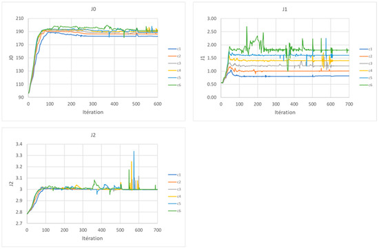
Figure 4.
Evolution of the cost function and the constraints for the constraint limits C1, C2, C3, C4, C5 and C6.
Table 5.
Cost function value for initial and final porous geometries for the constraint limits C1, C2, C3, C4, C5 and C6.
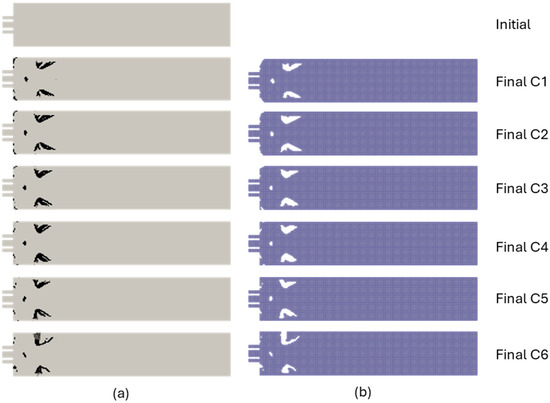
Figure 5.
Initial and final geometries for porous (a) and real (b) for the constraint limits C1, C2, C3, C4, C5 and C6.
To validate the optimal geometries, simulations are conducted using real wall boundary conditions. To accomplish this, the resulting geometries are extracted and meshes created for them, as illustrated in Figure 5b. The mesh consists of hexahedrons, each with sides of 1 mm. Close to the wall, the volume of the mesh elements is comparable to that of a 1 mm sided cube. Results are summarized in Table 6. The differences in cost function values between the final porous and real geometries are less than 4%.
Table 6.
Cost function value for initial and final real geometries for the constraint limits C1, C2, C3, C4, C5 and C6.
As illustrated in Figure 5 and Figure 6, the results show that to limit the production of the species , the algorithm creates deflectors that split the flow in two, thus creating a primary flux to feed reaction 1 (Equation (15)) and a secondary flux to dilute the flow, thereby limiting the temperatures and thus reaction 2 (Equation (16)). In Figure 5, the geometries are very similar. However, the analysis of the velocity fields, illustrated in Figure 7, shows that the slight differences in geometries naturally induce different velocity fields. Increasing the constraint limit results in a decrease in secondary flow speed. This reduction decreases the dilution effect, thereby increasing the temperature, as illustrated in Figure 8. The rise in temperature, as reaction kinetics are very sensitive to temperature levels, results in an increase in the chemical species and , as illustrated in Figure 9 and Figure 10. It is a straightforward illustration of the interest of objective optimization methods like the one developed in this work. These subtle differences in geometry and their relative qualities would be difficult to explore through intuitive or trial-and-error processes. Nevertheless, as recalled in the introduction, the secondary flow strategy is commonly used in modern gas turbines to limit the formation of nitrogen oxides.
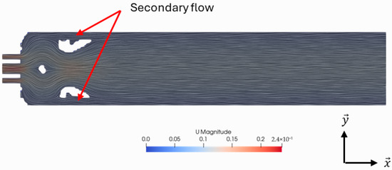
Figure 6.
Velocity field with streamlines for the final geometries with the constraint limits C1.
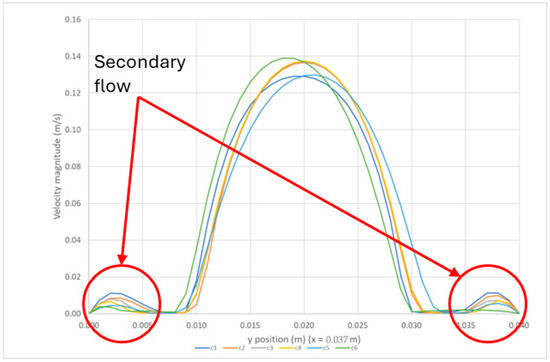
Figure 7.
Velocity as a function of at x = 37 mm.
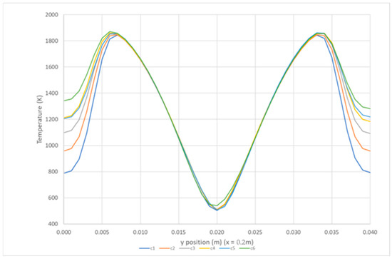
Figure 8.
Temperature as a function of y at x = 200 mm.
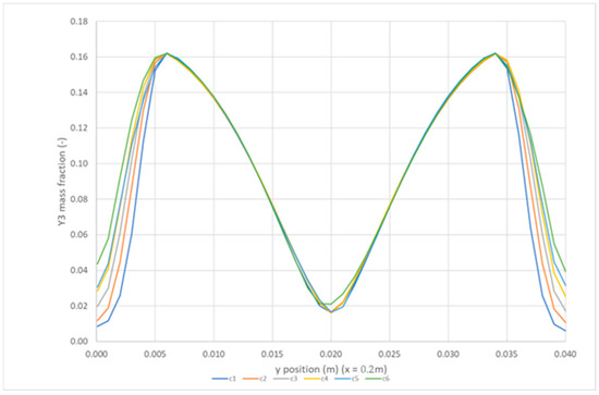
Figure 9.
mass fraction as a function of y at x = 200 mm.
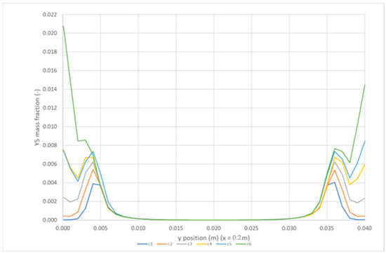
Figure 10.
mass fraction as a function of y at x = 200 mm.
4. Discussion
The gradient-based topology optimization method presented in this study demonstrates advances in optimizing reactive flows involving second-order chemical reactions. The density-based approach coupled with the adjoint method for gradient calculation proves particularly effective for maximizing desired reactions while constraining unwanted secondary reactions. With the gradient method, the challenge lies in accurately evaluating the gradient to ensure convergence toward the global optimum. The adjoint method is suitable to calculate the gradient, but without a reference, it is difficult to determine whether the obtained result is a global or local optimum. The absence of a robust reference benchmark means that, despite the accurate gradient direction, the optimization may still become trapped in a local minimum, particularly in problems with highly non-linear cost functions and constraints. However, Yoon [55] compares the sensitivity values of the finite difference method and the adjoint method on some cells. The result shows that the adjoint method provides the correct direction of the gradient. This reliability is essential for iterative schemes and helps ensure that the descent method follows a physically meaningful path. Furthermore, Yoshimura et al. [58] employed a genetic algorithm to solve the same problems addressed by Borrvall and Petersson [1], obtaining similar results. Therefore, the results provided by Borrvall and Petersson serve as reliable references for evaluating gradient methods in future work.
With the density method, the boundary layer may not be accurately calculated, as the porosity of the solid/fluid interface can result in residual flows different from usual Dirichlet boundary conditions, which can lead to poor results for turbulence problems. In laminar cases, Duan et al. [59] use a level set function with an adaptive mesh method, allowing the boundary layer to be calculated with high accuracy and achieving results similar to those of Borrvall and Petersson. Therefore, for laminar cases, it seems that the accuracy of the flow in the boundary layer is not an issue. For turbulent cases, it is known that the boundary layer plays an important role in the development of turbulence. Due to the bad representation of the boundary layer with the density method, it is possible that in turbulent cases, the density method and the level set method may find different optimal solutions, with an advantage for the level set method. Furthermore, incorporating more sophisticated turbulence models, such as Large Eddy Simulation (LES), into the topology optimization framework could help in high Reynolds number applications. In such flows, LES could better capture instantaneous turbulent structures and provide more accurate predictions, whereas the current approach might be limited by its reliance on laminar or averaged turbulence models.
Another important aspect is the computational cost associated with the presented methodology. The simulation times, particularly for problems involving chemical reaction optimization, may be substantial. While the MMA algorithm is robust and has been successfully applied to multiple cases, the overall computational burden highlights the need for improved efficiency. Strategies such as adaptive meshing and parallel computing could help reduce computational times while maintaining solution accuracy. Moreover, refining the adjoint system’s numerical implementation may also yield gains in efficiency, making the approach more viable for complex, industrial-scale problems. Nevertheless, the method computational performance should also be compared to other methods like heuristic developments. But due to the number of variable designs in topology optimization, the computational cost of these competitive methods is globally larger [58], particularly if one considers the risk presented by convergence to local optimums. Computational costs of laminar flows are known to be significantly lower for a given precision than turbulent. The method has therefore been adapted for laminar flows and illustrated for low Reynolds numbers in order to guarantee CFD convergence and precision. It should be effective in optimizing any reactive (second order) flow in a laminar regime. An interesting open question is to what extent the optimal geometry depends on turbulence intensity (Reynolds number) or other patterns of flow for a given objective. The answer requires extensive exploration of different configurations that the methodology exposed in this work makes possible.
Furthermore, the study does not explicitly address the robustness of optimized geometries under varying operational conditions. Real-world industrial environments typically exhibit fluctuations in boundary conditions, flow parameters, and chemical reaction rates. Assessing the sensitivity of optimized solutions to such variations is crucial for confirming their practical applicability and robustness. The current absence of sensitivity analysis or robustness validation constitutes a significant gap, limiting confidence in the practical reliability of the proposed optimization results. Also, the selection of penalty parameters during the optimization process may heavily influence the obtained geometries. While the two-step penalization strategy used aims to minimize local minima convergence, the determination of optimal penalty parameters remains somewhat arbitrary and might affect the final optimized solutions. Systematic studies to investigate the influence of penalty parameters on solution quality and convergence characteristics would enhance the method’s reliability and repeatability. The method’s practical applicability and reliability could be significantly enhanced by addressing these limitations, including robustness under variable conditions and systematic parameter sensitivity assessments. Addressing these concerns will substantially strengthen confidence and industrial relevance of the proposed optimization framework.
5. Summary and Outlook
A robust adjoint-based gradient calculation method integrated into a density-based topology optimization framework to optimize reactive fluid flows involving second-order chemical reactions has been described. Validation using the classical bend-pipe case confirmed the reliability of the optimization procedure. Application to second-order reactive flows led to substantial improvements, with the optimized configurations significantly enhancing the reaction efficiency while effectively limiting unwanted secondary reactions. Specifically, the optimization achieved first-reaction efficiency gains of up to 98.7% in porous geometries and 105.2% in real geometries. The resulting geometries adopted flow-splitting strategies analogous to techniques used in modern gas turbine designs, validating both the method’s practicality and its alignment with industrial practices. Initially, the calculations utilized a Reynolds number of 1; however, higher Reynolds numbers can be employed as long as the flow remains laminar. It is crucial to highlight that the Reynolds number significantly affects the optimal geometry, similar to its impact on power dissipation in a bent pipe. Future developments will focus on evaluating the impact of high Reynolds numbers on the optimal geometries in the laminar case and extending the approach to turbulent regimes by integrating advanced turbulence modeling techniques, such as Large Eddy Simulation, to tackle more complex industrial applications.
Moreover, hybrid optimization strategies combining density and level-set approaches will be explored to further enhance the precision and applicability of topology optimization in fluid dynamics.
Author Contributions
Conceptualization, H.P. and L.L.M.; methodology, H.P. and L.L.M.; software, H.P.; validation, H.P., L.L.M., J.J. and N.S.; formal analysis, H.P.; investigation, H.P.; resources, H.P.; data curation, H.P.; writing—original draft preparation, H.P.; writing—review and editing, H.P., L.L.M., J.J. and N.S.; visualization, H.P.; supervision, L.L.M.; project administration, L.L.M.; funding acquisition, L.L.M. All authors have read and agreed to the published version of the manuscript.
Funding
This research received no external funding and The APC was funded by l’Université Bourgogne Europe.
Data Availability Statement
The raw data supporting the conclusions of this article will be made available by the authors on request.
Conflicts of Interest
The authors declare no conflict of interest.
List of Symbols
| Design variable | |
| Design vector | |
| Cost function/constraint | |
| Constraint | |
| Volume of the study domain | |
| Boundary of the study domain | |
| Nabal/gradient operator | |
| Identity matrix | |
| Density | |
| Time | |
| Velocity vector | |
| Pressure, or descent step | |
| Chemical specie | |
| Mass fraction of the chemical species | |
| Viscous stress tensor | |
| Inverse permeability field | |
| Penalization parameter | |
| Descent direction | |
| Lagrangian | |
| , , | Vector of Lagrange multipliers |
| Lagrange multiplier | |
| Kinematic viscosity | |
| Diffusion coefficient | |
| Thermal diffusivity | |
| Constant reaction rate | |
| Enthalpy of reaction | |
| Heat capacity |
Appendix A
Appendix A.1. Gradients of Cost Function and Constraints
Appendix A.2. Adjoint Systems
, and are also components of the vector of Lagrange multipliers. The boundary conditions associated with the adjoint systems are as follows:
where subscripts and indicate the tangential and normal components, respectively.
References
- Junejo, A.; Al-Abdeli, Y.M.; Porteiro, J. Role of Air Staging in a Batch-Type Fixed Bed Biomass Combustor under Constant Primary Air. J. Therm. Sci. 2024, 33, 284–299. [Google Scholar] [CrossRef]
- Tu, Y.; Zhang, H.; Guiberti, T.F.; Avila Jimenez, C.D.; Liu, H.; Roberts, W.L. Experimental and numerical study of combustion and emission characteristics of NH3/CH4/air premixed swirling flames with air-staging in a model combustor. Appl. Energy 2024, 367, 123370. [Google Scholar] [CrossRef]
- Srinivasarao, M.; Kumar, S.; Jik Lee, B.; Giri, B.R.; Shrestha, K.P.; Mahendra Reddy, V. Experimental and numerical analysis on influence of air staging in a tangential flow burner for pure ammonia combustion. Appl. Therm. Eng. 2025, 266, 125580. [Google Scholar] [CrossRef]
- Borrvall, T.; Petersson, J. Topology optimization of fluids in Stokes flow. Int. J. Numer. Methods Fluids 2003, 41, 77–107. [Google Scholar] [CrossRef]
- Alexandersen, J.; Andreasen, C.S. A Review of Topology Optimisation for Fluid-Based Problems. Fluids 2020, 5, 29. [Google Scholar] [CrossRef]
- Li, H.; Wang, C.; Zhang, X.; Li, J.; Shen, J.; Zhou, S. A Mini Review on Fluid Topology Optimization. Materials 2023, 16, 6073. [Google Scholar] [CrossRef]
- Abdel Nour, W.; Jabbour, J.; Serret, D.; Meliga, P.; Hachem, E. A Stabilized Finite Element Framework for Anisotropic Adaptive Topology Optimization of Incompressible Fluid Flows. Fluids 2023, 8, 232. [Google Scholar] [CrossRef]
- Liu, J.; Li, R.; Chen, Y.; Zheng, J.; Wang, K. Topology Optimization Method of a Cavity Receiver and Built-In Net-Based Flow Channels for a Solar Parabolic Dish Collector. Entropy 2023, 25, 398. [Google Scholar] [CrossRef]
- Zhao, N.; Zhang, J.; Han, H.; Miao, Y.; Deng, Y. Topology Optimization of Hydrodynamic Body Shape for Drag Reduction in Low Reynolds Number Based on Variable Density Method. Appl. Sci. 2023, 13, 5461. [Google Scholar] [CrossRef]
- Okkels, F.; Bruus, H. Scaling behavior of optimally structured catalytic microfluidic reactors. Phys. Rev. E 2007, 75, 16301. [Google Scholar] [CrossRef]
- Okkels, F.; Bruus, H. Design of Micro-Fluidic Bio-Reactors Using Topology Optimization. J. Comput. Theor. Nanosci. 2007, 4, 814–816. [Google Scholar] [CrossRef][Green Version]
- Schäpper, D.; Lencastre Fernandes, R.; Lantz, A.E.; Okkels, F.; Bruus, H.; Gernaey, K.V. Topology optimized microbioreactors. Biotechnol. Bioeng. 2011, 108, 786–796. [Google Scholar] [CrossRef]
- Yaji, K.; Yamasaki, S.; Tsushima, S.; Suzuki, T.; Fujita, K. Topology optimization for the design of flow fields in a redox flow battery. Struct. Multidiscip. Optim. 2018, 57, 535–546. [Google Scholar] [CrossRef]
- Behrou, R.; Pizzolato, A.; Forner-Cuenca, A. Topology optimization as a powerful tool to design advanced PEMFCs flow fields. Int. J. Heat Mass Transf. 2019, 135, 72–92. [Google Scholar] [CrossRef]
- Dugast, F.; Favennec, Y.; Josset, C. Reactive fluid flow topology optimization with the multi-relaxation time lattice Boltzmann method and a level-set function. J. Comput. Phys. 2020, 409, 109252. [Google Scholar] [CrossRef]
- Liu, X.; Chen, L.; Tao, W.-Q. Effects of physicochemical parameters on the optimized topology of catalyst in micro reactors. Front. Heat Mass Transf. 2020, 14, 1–9. [Google Scholar] [CrossRef]
- Jia, S.; Cao, X.; Yuan, X.; Yu, K.-T. Multi-objective topology optimization for the solar thermal decomposition of methane reactor enhancement. Chem. Eng. Sci. 2021, 231, 116265. [Google Scholar] [CrossRef]
- Bhattacharjee, D.; Atta, A. Topology optimization of a packed bed microreactor involving pressure driven non-Newtonian fluids. React. Chem. Eng. 2022, 7, 609–618. [Google Scholar] [CrossRef]
- Wang, J.; Wang, Y.; Ma, L.; Liu, X. Multi-objective topology optimization and flow characteristics study of the microfluidic reactor. React. Kinet. Mech. Catal. 2022, 135, 2475–2501. [Google Scholar] [CrossRef]
- Guo, C.; Chen, L.; Tao, W. Topology optimization of microreactors for hydrogen production by ammonia catalytic decomposition. Int. J. Hydrogen Energy 2024, 96, 923–937. [Google Scholar] [CrossRef]
- Sigmund, O.; Petersson, J. Numerical instabilities in topology optimization: A survey on procedures dealing with checkerboards, mesh-dependencies and local minima. Struct. Optim. 1998, 16, 68–75. [Google Scholar] [CrossRef]
- Zuo, K.-T.; Chen, L.-P.; Zhang, Y.-Q.; Yang, J. Study of key algorithms in topology optimization. Int. J. Adv. Manuf. Technol. 2007, 32, 787–796. [Google Scholar] [CrossRef]
- Bendsøe, M.P. Optimal shape design as a material distribution problem. Struct. Optim. 1989, 1, 193–202. [Google Scholar] [CrossRef]
- Zhou, M.; Rozvany, G.I.N. The COC algorithm, Part II: Topological, geometrical and generalized shape optimization. Comput. Methods Appl. Mech. Eng. 1991, 89, 309–336. [Google Scholar] [CrossRef]
- Mlejnek, H.P. Some aspects of the genesis of structures. Struct. Optim. 1992, 5, 64–69. [Google Scholar] [CrossRef]
- Sigmund, O.; Maute, K. Topology optimization approaches: A comparative review. Struct. Multidiscip. Optim. 2013, 48, 1031–1055. [Google Scholar] [CrossRef]
- Eberhart, R.; Kennedy, J. A new optimizer using particle swarm theory. In Proceedings of the Sixth International Symposium on Micro Machine and Human Science (MHS’95), Nagoya, Japan, 4–6 October 1995; IEEE: New York, NY, USA, 1995; pp. 39–43. [Google Scholar]
- Wu, X.; Han, J.; Wang, D.; Gao, P.; Cui, Q.; Chen, L.; Liang, Y.; Huang, H.; Lee, H.P.; Miao, C.; et al. Incorporating Surprisingly Popular Algorithm and Euclidean distance-based adaptive topology into PSO. Swarm Evol. Comput. 2023, 76, 101222. [Google Scholar] [CrossRef]
- Luh, G.-C.; Lin, C.-Y.; Lin, Y.-S. A binary particle swarm optimization for continuum structural topology optimization. Appl. Soft Comput. 2011, 11, 2833–2844. [Google Scholar] [CrossRef]
- Najafabadi, H.R.; Goto, T.; Falheiro, M.; Martins, T.C.; Barari, A.; Tsuzuki, M.S.G. Post-Processing of non gradient-based Topology Optimization with Simulated Annealing. IFAC-PapersOnLine 2021, 54, 755–760. [Google Scholar] [CrossRef]
- Kirkpatrick, S.; Gelatt, C.D.; Vecchi, M.P. Optimization by simulated annealing. Science 1983, 220, 671–680. [Google Scholar] [CrossRef]
- Černý, V. Thermodynamical approach to the traveling salesman problem: An efficient simulation algorithm. J. Optim. Theory Appl. 1985, 45, 41–51. [Google Scholar] [CrossRef]
- Kaveh, A.; Hassani, B.; Shojaee, S.; Tavakkoli, S.M. Structural topology optimization using ant colony methodology. Eng. Struct. 2008, 30, 2559–2565. [Google Scholar] [CrossRef]
- Yoo, K.-S.; Han, S.-Y. A modified ant colony optimization algorithm for dynamic topology optimization. Comput. Struct. 2013, 123, 68–78. [Google Scholar] [CrossRef]
- Lee, K.S.; Geem, Z.W. A new structural optimization method based on the harmony search algorithm. Comput. Struct. 2004, 82, 781–798. [Google Scholar] [CrossRef]
- Qin, F.; Zain, A.M.; Zhou, K.-Q. Harmony search algorithm and related variants: A systematic review. Swarm Evol. Comput. 2022, 74, 101126. [Google Scholar] [CrossRef]
- Storn, R.; Price, K. Differential Evolution—A simple and efficient adaptive scheme for global optimization over continuous spaces. J. Glob. Optim. 1995, 11, 341–359. [Google Scholar] [CrossRef]
- Storn, R. Differential Evolution—A Simple and Efficient Heuristic for Global Optimization over Continuous Spaces. Differ. Evol. 1997, 11, 341–359. [Google Scholar] [CrossRef]
- Wu, C.-Y.; Tseng, K.-Y. Topology optimization of structures using modified binary differential evolution. Struct. Multidiscip. Optim. 2010, 42, 939–953. [Google Scholar] [CrossRef]
- Luh, G.-C.; Chueh, C.-H. Multi-modal topological optimization of structure using immune algorithm. Comput. Methods Appl. Mech. Eng. 2004, 193, 4035–4055. [Google Scholar] [CrossRef]
- Xie, Y.M.; Steven, G.P. A simple evolutionary procedure for structural optimization. Comput. Struct. 1993, 49, 885–896. [Google Scholar] [CrossRef]
- Young, V.; Querin, O.M.; Steven, G.P.; Xie, Y.M. 3D and multiple load case bi-directional evolutionary structural optimization (BESO). Struct. Optim. 1999, 18, 183–192. [Google Scholar] [CrossRef]
- Jakiela, M.J.; Chapman, C.; Duda, J.; Adewuya, A.; Saitou, K. Continuum structural topology design with genetic algorithms. Comput. Methods Appl. Mech. Eng. 2000, 186, 339–356. [Google Scholar] [CrossRef]
- Chapman, C.D. Structural Topology Optimization via the Genetic Algorithm. Master’s Thesis, Massachusetts Institute of Technology, Department of Mechanical Engineering, Cambridge, MA, USA, 1994. [Google Scholar]
- Holland, J. Adaptation in Natural and Artificial System; University of Michigan Press: Ann Arbor, MI, USA, 1975. [Google Scholar]
- Kicinger, R.; Arciszewski, T.; Jong, K.D. Evolutionary computation and structural design: A survey of the state-of-the-art. Comput. Struct. 2005, 83, 1943–1978. [Google Scholar] [CrossRef]
- Sigmund, O. On the usefulness of non-gradient approaches in topology optimization. Struct. Multidiscip. Optim. 2011, 43, 589–596. [Google Scholar] [CrossRef]
- Gilbert, J.C. Optimisation Différentiable; AF1252 V1; Techniques de l’ingénieur: Saint-Denis, France, 2008. [Google Scholar] [CrossRef]
- Cauchy, M.A. Méthode générale pour la résolution des systèmes d’équations simultanées. Comp. Rend. Sci. Paris 1847, 25, 536–538. [Google Scholar]
- Fleury, C. CONLIN: An efficient dual optimizer based on convex approximation concepts. Struct. Optim. 1989, 1, 81–89. [Google Scholar] [CrossRef]
- Svanberg, K. The method of moving asymptotes—A new method for structural optimization. Int. J. Numer. Methods Eng. 1987, 24, 359–373. [Google Scholar] [CrossRef]
- Svanberg, K. A Class of Globally Convergent Optimization Methods Based on Conservative Convex Separable Approximations. SIAM J. Optim. 2002, 12, 555–573. [Google Scholar] [CrossRef]
- Giles, M.B.; Pierce, N.B. An introduction to the adjoint approach to design. Flow Turbul. Combust. 2000, 65, 393–415. [Google Scholar] [CrossRef]
- Bradley, A.M. PDE-Constrained Optimization and the Adjoint Method. 2010. Available online: https://cs.stanford.edu/~ambrad/adjoint_tutorial.pdf (accessed on 10 August 2025).
- Yoon, G.H. Topology optimization method with finite elements based on the k- ε turbulence model. Comput. Methods Appl. Mech. Eng. 2020, 361, 112784. [Google Scholar] [CrossRef]
- Yoon, G.H. Topology optimization for turbulent flow with Spalart–Allmaras model. Comput. Methods Appl. Mech. Eng. 2016, 303, 288–311. [Google Scholar] [CrossRef]
- Na, J.; Li, H.; Yan, P.; Li, X.; Gao, X. An open-source topology optimization modeling framework for the design of passive micromixer structure. Chem. Eng. Sci. 2022, 259, 117820. [Google Scholar] [CrossRef]
- Yoshimura, M.; Shimoyama, K.; Misaka, T.; Obayashi, S. Topology optimization of fluid problems using genetic algorithm assisted by the Kriging model: Topology optimization using a kriging-based genetic algorithm. Int. J. Numer. Methods Eng. 2017, 109, 514–532. [Google Scholar] [CrossRef]
- Duan, X.; Li, F.; Qin, X. Topology optimization of incompressible Navier–Stokes problem by level set based adaptive mesh method. Comput. Math. Appl. 2016, 72, 1131–1141. [Google Scholar] [CrossRef]


Disclaimer/Publisher’s Note: The statements, opinions and data contained in all publications are solely those of the individual author(s) and contributor(s) and not of MDPI and/or the editor(s). MDPI and/or the editor(s) disclaim responsibility for any injury to people or property resulting from any ideas, methods, instructions or products referred to in the content. |
© 2025 by the authors. Licensee MDPI, Basel, Switzerland. This article is an open access article distributed under the terms and conditions of the Creative Commons Attribution (CC BY) license (https://creativecommons.org/licenses/by/4.0/).