Abstract
This paper addresses the problem of the design optimization of turbomachinery components under thermo-mechanical constraints, with focus on a radial turbine impeller for turbocharger applications. Typically, turbine components operate at high temperatures and are exposed to important thermal gradients, leading to thermal stresses. Dealing with such structural requirements necessitates the optimization algorithms to operate a coupling between fluid and structural solvers that is computationally intensive. To reduce the cost during the optimization, a novel multiphysics gradient-based approach is developed in this work, integrating a Conjugate Heat Transfer procedure by means of a partitioned coupling technique. The discrete adjoint framework allows for the efficient computation of the gradients of the thermo-mechanical constraint with respect to a large number of design variables. The contribution of the thermal strains to the sensitivities of the cost function extends the multidisciplinary outlook of the optimization and the accuracy of its predictions, with the aim of reducing the empirical safety factors applied to the design process. Finally, a turbine impeller is analyzed in a demanding operative condition and the gradient information results in a perturbation of the grid coordinates, reducing the stresses at the rotor back-plate, as a demonstration of the suitability of the presented method.
1. Introduction
Multidisciplinary optimization methods are widely adopted in the development cycle of turbomachinery-related technologies, such as in the energy and mobility businesses [1,2,3]. The increasing complexity of the products in terms of geometry and flow characteristics in design and off-design conditions, along with the fulfillment of requirements of lifetime, cost, and packaging, is reflected in the growth of concurrent design techniques that provide the experts with a comprehensive view on the problem [4,5]. The exploration of the design space is enriched by multiple physical disciplines whose interactions are captured along the optimization, resulting in accurate predictions of the component performance and any possible violation of the structural constraints. This holistic approach to the design problem differs from classical staggered methods, presenting a series of mono-discipline optimizations performed in cascade, leading typically to significantly longer development times. Moreover, such staggered methods may not converge to the same optimum as the holistic one and thus lead to suboptimal designs.
1.1. Background
The recent evolution of the market request towards aggressive reductions in emissions and fuel consumption offers new challenges to the research community. The need for further advances in multidisciplinary design optimization techniques is presented in the NASA 2040 roadmap [6] as one of nine core development areas in the context of integrated multiscale modelling frameworks contributing to the success in efficient design, manufacturing, and certification of future aerospace systems. Similarly, the engineering of advanced turbocharging solutions in the automotive sector demands further increases in efficiency to support novel combustion strategies, with no compromise on the durability targets [7,8].
Enhancements in turbomachinery components performance can be achieved by increasing the detail in the geometrical representation of the domain and reflecting it in a higher number of parameters engaged during the optimization process. This higher resolution allows the exploration of more complex shapes and discloses hidden interactions among features now present in the design space. Additionally, an increased fidelity in the physical description of the multidisciplinary problem is highly regarded and the aim is twofold. First, the optimizer is able to make more reliable predictions of the responses to the geometrical modifications, having access to lumped information accounting for the interactions of more disciplines involved in the computation of the objective functions and constraints. Therefore, the evolution of the optimization benefits from adhering more to the real behavior of the component, finally resulting in a reduced amount of experimental validation testing. Second, a more sophisticated physical description opens the path to adopting a richer set of constraints, and the safety margins usually applied to the design process can be relaxed in favor of more performance-oriented layout choices. Therefore, the optimizer can target more diversified paths towards the achievement of the desired solution, thus reducing the stiffness of the algorithm in performing the shape modifications.
The increased complexity in the models is reflected in the choice of a suitable optimization method between two major classes, notably denoted as gradient-free and gradient-based techniques.
Gradient-free methods [9], also known as “zero-order” methods, solely make use of the function values for the search of the global optimum, neglecting any knowledge of its gradients. The solution is identified after the evaluation of the output values of a large population of candidates with characteristics scattered within the boundaries of the selected design space. The larger the population, the higher the likelihood of identifying the global optimum. In the case of a multidisciplinary problem, each sample in the population must be processed through all the disciplines (FEM and FVM analyses, among others) [10]. Therefore, the number of computations necessary to identify a solution scales up with the number of involved disciplines and the number of design variables necessary to investigate the full domain, resulting quickly in a computationally expensive approach [11,12]. Even if, nowadays, gradient-free methods still represent the state-of-the-art approach to optimizations in industry because of their robustness and the high quality of the solutions, the advent of more stringent requirements and the need of evaluating larger domains are exposing an intrinsic limitation, notably referred to as the “curse of dimensionality” [13].
Gradient-based methods [14,15], with specific reference to “first-order” methods, make use of the gradient information of the function of interest in the search of the optimal solution, and therefore are more efficient than zero-order methods. The evaluation of the gradients may be computationally intensive if performed by Finite Differences or complex step techniques [16], especially in the presence of a large number of design variables and in the case of disciplines involving expensive computations. However, if the number of objective functions is lower than the number of optimization parameters, an efficient calculation of the gradients can be obtained by the adjoint method [17]. This technique, first introduced in [18] for fluid problems, is characterized by a cost for the computation of the sensitivity derivatives of the objective function that is essentially independent of the number of design variables. Therefore, it is particularly suited for problems requiring detailed geometrical descriptions with many degrees of freedom. Moreover, the exploration of the design space through its gradients decreases the number of iterations necessary to achieve the local optimal solution. Therefore, the reduced overhead can be traded for the introduction of more computationally demanding disciplines, returning a higher accuracy in the numerical solutions.
A performance comparison between these two techniques is offered in [19], whose application to the multi-point optimization of a radial turbine impeller shows that the adjoint method is capable of extending the Pareto front identified by a differential evolution (DE) algorithm. In particular, the gradient-based approach delivers a solution with a higher total-to-static efficiency, improving also the moment of inertia figure at the cost of a fraction of the computational time required by the gradient-free method to achieve its global optimum (roughly 6–10%). Other examples of applications of the adjoint methods to the optimization of turbines and compressors are reported in [20,21,22,23,24,25], with focus on the opportunity of increasing the number of variables in the design space and the multidisciplinary aspect of the physical evaluations (including aerodynamics, stresses, and modal analysis).
The higher maturity recently gained by gradient-based approaches and their improved robustness in the analysis of complex flow conditions [26,27] provides evidence of their application to problems of industrial relevance. Therefore, adjoint methods are considered a suitable choice to address the previously mentioned design advancements in turbomachinery-related applications.
1.2. Motivation
The present document focuses on the development of a radial turbine impeller for an automotive turbocharger. In contrast to aeronautical applications, the typical duty cycles for passenger cars span the entire turbine map, from very low mass flow rates and pressure ratios in urban driving situations up to peak power, resulting in requirements stretching the machine design over a wide range of operative conditions. Moreover, these turbines present tight clearances between rotor and housing in the order of few hundreds of microns, whilst the typical thermal operative range spans from ambient temperature up to 1050 °C, without the possibility of any blade-dedicated cooling circuit. Such scenario clearly demonstrates the challenges in performance requirements and durability the designer is confronted with during the product development process.
The structural integrity of the rotor experiencing centrifugal and fluid-induced stresses is a critical aspect in the search for design solutions fulfilling the efficiency and permeability targets. The problem of the Fluid–Structure Interaction (FSI) in radial turbines in relation to the thermal stresses induced by the fluid in contact with the blades is discussed in [28], in an effort to accurately predict the heat exchange between the two media for a reliable estimation of the rotor lifetime in steady state and dynamic operative conditions. The study shows how the incorrect estimation of the thermal stresses could impair the robustness of the component, justifying the inclusion of this additional constraint on top of the computation of the centrifugal stresses.
The introduction of thermal analyses in the framework of an optimization process is a topic of recent interest [29,30,31]. The physical phenomenon is described through the application of a Conjugate Heat Transfer (CHT) procedure, as originally proposed in [32,33], which involves the thermal interaction between a solid body and its surrounding fluid by a coupled solution of the two domains. The challenge in the implementation of this analysis within the landscape of a multidisciplinary optimization of a complex geometry consists of the trade-off between accuracy and significant computational overhead, so far limiting thermal predictions only to the final validation phase in industrial design procedures. In fact, it is common practice during an optimization to replace such intensive computations with reduced-order models or safety margins based on empirical experience. This approach to the evaluation of the thermal stresses would suffer in terms of accuracy or, in the case of large safety margins, would over-constrain the optimization problem.
1.3. Goal of the Paper
This paper addresses the problem of robust optimizations w.r.t. thermo-mechanical stresses by developing a discrete adjoint framework tailored to the implementation of the CHT analysis within the in-house multidisciplinary design and optimization platform “CADO” developed at the von Karman Institute for Fluid Dynamics [34]. Indeed, the selection of a gradient-based method is justified by its computational efficiency in identifying a local minimum, although the computation of the gradients is more convoluted due to the multiple disciplines involved in the performance analysis. The calculation of the thermal stresses in the solid domain and their sensitivities with respect to the grid coordinates is therefore the subject of the present paper, with the aim of including this analysis in a Sequential Quadratic Programming-based optimizer [35].
To the best of our knowledge, only a few studies have considered the CHT analysis in adjoint-based optimizations [36,37], with only a limited number adopting a discrete adjoint formulation [38,39,40] and none treating a test case with a complex three-dimensional flow field or extending the problem to thermo-mechanical evaluations. Therefore, this work is aimed at covering critical gaps in the design of radial turbines with the aim of creating a framework suitable for industrial applications.
In light of this objective, the remaining portion of the document is structured as follows. First, the framework of the primal solver for the execution of the CHT analysis is presented, with extension to the computation of the thermo-mechanical stresses. Then, the implementation of the adjoint workflow for the calculation of the sensitivities of the constraint function with respect to the solid and fluid grid coordinates is discussed, outlining the steps towards the coupling of the domains in reverse mode. Finally, the validation of the model and the results of the application of the procedure to a radial turbine rotor test case are presented and the conclusions are drawn from this study.
2. Primal Solver
The CHT analysis implemented in the current work follows the partitioned coupling approach proposed by [41], in which a fluid and a solid solver are sequentially called in an iterative process with the mutual exchange of boundary conditions till reaching the convergence of the temperature at their interface. The advantage of this strategy is related to the possibility of adopting dedicated meshes and specialized numerical methods for the solution of each domain, increasing the robustness of the convergence of the two analyses. Moreover, in the case of an unsteady computation, the partial decoupling of the two fields, which show very different characteristic time scales, would lead to a faster convergence of the assembly [42,43,44,45].
2.1. Mapping Procedure
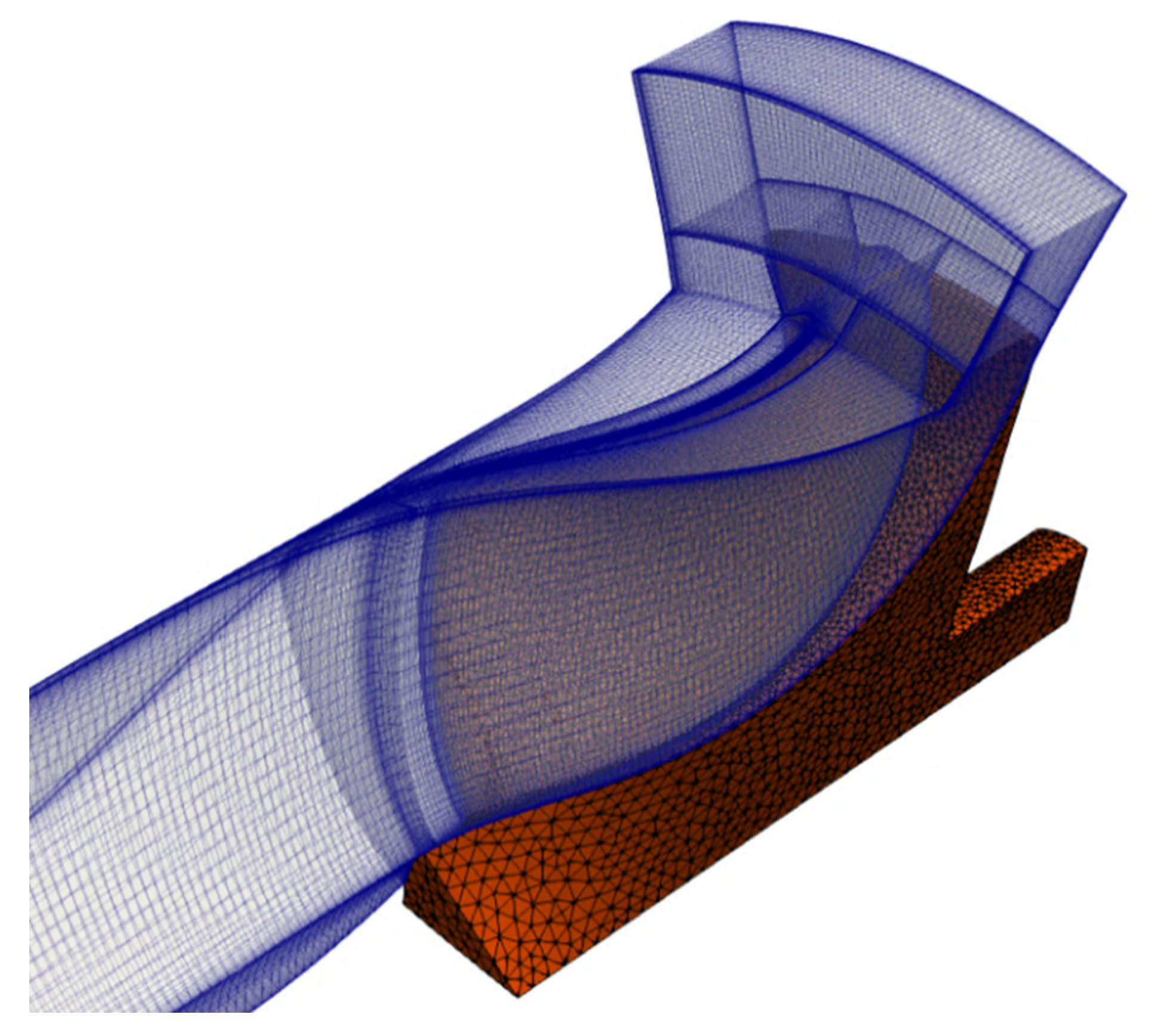
The problem under investigation is represented in Figure 1, in which a turbine rotor is analyzed considering a periodic sector. A multi-block structured fluid grid with boundary layer refinement is interfaced to an unstructured solid mesh of second-order tetrahedral elements for the computation of the heat flux between the two domains.

Figure 1.
Radial turbine rotor: fluid and solid sector meshes.
Because the meshes are non-matching at the common interface, the exchange of information is performed through the distance-weighted interpolation (DWI) technique presented in [46]. The procedure implies the mapping of the two regions in order to record the correspondences of each fluid cell center with the closest surrounding solid nodes and vice versa. For each fluid cell, the information of heat flux or temperature detected in the mating solid nodes is processed by a weighting function based on their mutual distances, resulting in the coupling of the two regions. The same routine is applied to the solid grid with respect to its fluid counterpart.
This method exhibits a good level of generality in treating different coupling problems, irrespective of their grids characteristics. For instance, in the turbine test case the exchange of information is effectively performed also at the blade hub fillet, a feature which is present in the solid domain but not detailed in the corresponding fluid region.
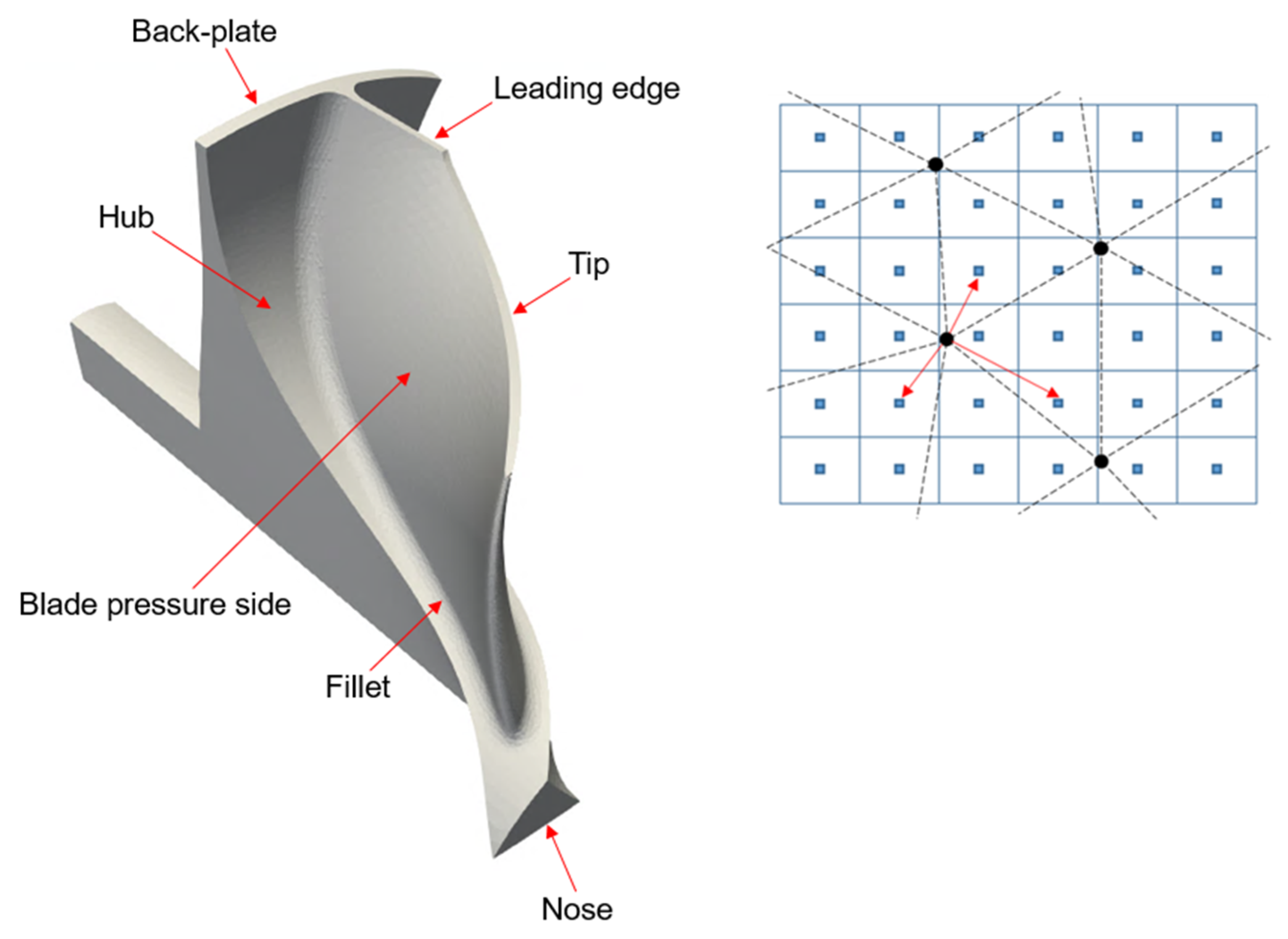
An improvement in the accuracy of this coupling procedure derives from the local labelling of the interface. With reference to Figure 2, the surface between the two media is split in sub-regions (e.g., hub, blade pressure side, blade suction side, tip, etc.) and the corresponding solid faces and fluid blocks boundaries are named accordingly. Therefore, the algorithm searching for the fluid cells–solid nodes correspondences is separately executed for each sub-region, instead of attempting the coupling of the two fields through a global search within the entire domain. This arrangement is particularly effective in locations presenting thin walls, such as in proximity of the blade tip, as it avoids any erroneous fluid-solid matching between cells and nodes actually sitting on opposite sides of the blade (i.e., suction side versus pressure side).
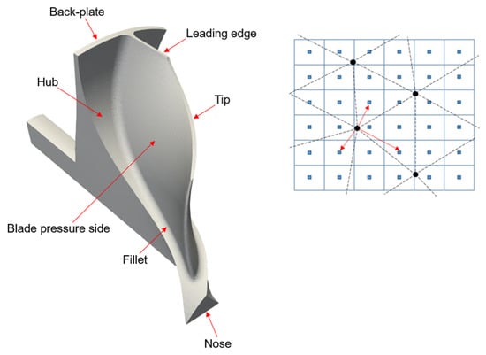
Figure 2.
Radial turbine rotor surface split in sub-regions (left), example of FVM-FEM meshes correspondence identification (right).
Additionally, the original algorithm seeks the nodes–cells correspondences through a “search radius” delimiting for each grid node a spherical volume within which the neighbors are identified. This technique may induce interpolation errors in proximity of the walls, where temperature gradients and fluid grid stretching are significant. In fact, the temperature assigned to a solid node may result from the weighting of temperature values derived from fluid cells located within the boundary layer but not in direct contact with the interface. Moreover, as demonstrated in [46], distinct grid refinements at the solid and fluid side may influence the local accuracy of the wall temperature information passed to the FEM. In order to cope with these issues, the searching criterion is limited to the sole layer of nodes and cells in direct contact with the walls, and the concept of “search radius” is dismissed in favor of a ranking assigned to each node or cell according to their mutual distance. Finally, consistently with the solution proposed in [46] addressing the problem of the aspect ratio of cells on a wall boundary, additional virtual grid points are introduced on the FVM side between two neighboring cell centers. Such virtual points are aimed at improving the uniformity of the local distribution of grid points in regions of significant mesh stretching, and their temperature is interpolated between the closest “master” cells of the original mesh. Indeed, the goal is to increase the density of the attractors in proximity of each solid node, avoiding possible inconsistencies generated from capturing the information from too far fluid cells. Thus, the domain coupling is executed through the distance-weighting interpolation of information belonging to cells and nodes in actual close proximity.
The quality of the interpolation is referenced in Figure 3. The fluid temperature at the walls (Figure 3a) is interpolated by the DWI procedure and passed to the solid nodes laying on the surface (Figure 3b). During a CHT iteration, the solid returns the heat flux to the fluid, as discussed in the next section.
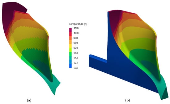
Figure 3.
Distance-weighted interpolation method applied to the exchange of information between solid and fluid domains: (a) fluid temperature at walls, (b) interpolated fluid temperature assigned to the solid surface.
2.2. Partitioned Coupling
The data exchange between the fluid and solid fields is performed through the “heat transfer forward flux back” method (hFFB) [47], whose stability properties are discussed in [48]. In summary, the convergence rate of the conjugate problem depends on the local Biot number, which expresses the ratio between the conductive over the convective thermal resistances. In complex geometries, as in the case of a radial turbine impeller, the Biot number may locally change to values greater or lower than unity, according to the variations in the blade thickness. Hence, [46] demonstrates that methods such as the hFFB or the “heat transfer forward temperature back” (hFTB) method would promote the stabilization of the fluid-solid coupling w.r.t. other techniques, such as the “flux forward temperature back” (FFTB) or the “temperature forward flux back” (TFFB) methods, which strictly require a modulus of the Biot number respectively lower or greater than unity. Instead, the hFTB and hFFB methods exhibit a wider range of convergence. Finally, the hFFB method was selected for the present study since a heat flux boundary condition imposed to the fluid domain would generally improve the convergence stability of the CFD computation more than an imposed wall temperature boundary condition.
Figure 4 reports the partitioned coupling workflow, described as follows.
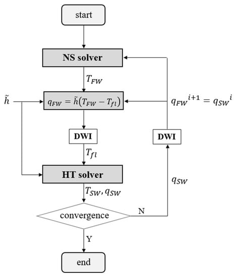
Figure 4.
hFFB coupling method for the CHT analysis.
The CHT analysis is addressed with an initial CFD computation considering adiabatic walls. The fluid temperature and the heat flux normal to the walls are extracted at the boundaries in contact with the solid, and a virtual fluid bulk temperature is calculated as:
with indicating a constant user-defined virtual heat transfer coefficient.
Since the initial fluid simulation is adiabatic, Equation (1) results in a virtual fluid bulk temperature equal to the fluid temperature at the walls. The DWI procedure returns the field associated with the solid grid nodes.
Consequently, and are assigned to the FEM heat transfer model, such that the heat flux to the solid results from the following boundary condition:
with T as the unknown solid temperature. After solving the FEM heat transfer problem, the temperature and heat flux at this boundary are known.
The heat flux at the interface is calculated from the temperature field T by means of the Fourier’s law applied to all the elements exposing at least one face to the fluid:
with indicating the temperature gradient normal to the wall and k the thermal conductivity coefficient.
The heat flux is processed by the DWI procedure, returning the heat flux assigned to the fluid cells at the interface. The fluid simulation, now accounting for an external heat flux at the viscous walls, is recomputed and the entire process is re-iterated for several loops till the achievement of the continuity of temperatures at the interface between the two fields.
The user-imposed virtual heat transfer coefficient influences the predicted wall heat fluxes at any intermediate cycle of the CHT procedure, thus determining the path to convergence of the whole coupling. In the case of the hFFB method, [46] shows that a suitable choice of the virtual coefficient , with h as the physical value of the heat transfer coefficient, would guarantee the convergence of the conjugate problem for any local value of the Biot number. The higher the value of within the stable region, the faster the convergence of the partitioned coupling method. A discussion about the determination of the value for a problem of industrial relevance is reported in Section 4.2.
2.3. Solid Heat Transfer Solver
The steady-state energy balance within the solid domain is described by Equation (4), with q as the rate of heat transfer into the system, and is computed through a FEM steady linear solver according to [49].
The boundary conditions applied to the problem are classified in three families:
with the surface of the solid domain defined as .
The first equation in (5) implies a fixed temperature imposed at the surface The second type of boundary conditions specifies a heat flux at the surface , while Fourier’s law at LHS describes the heat flux through the medium. If q = 0, the adiabatic wall boundary condition is defined. The third equation represents the convection condition, whose heat flux through the surface is proportional to the temperature difference w.r.t. the surrounding fluid. The virtual heat transfer coefficient and the interpolated thermal field are reported for the sake of consistency with Equation (2).
Once integrated over the entire domain, Equation (4) is discretized, resulting in the linear system:
with the semi-positive definite stiffness matrix A comprising the conductive and convective terms, A = [Acond + Aconv] , and the load vector b accounting for the contribution of the boundary conditions. The linear system in (6) is solved by an iterative conjugate gradient method.
2.4. Fluid Solver
The compressible Reynolds-Averaged Navier–Stokes solver with cell-centered spatial discretization over a structured multi-block grid, developed in [19], is invoked in the CHT framework. The solver computes the convective fluxes by Roe’s upwind scheme with MUSCL extrapolation, while a central discretization is applied to the calculation of viscous fluxes. The time marching technique is implemented according to the JT-KIRK scheme proposed in [26] for the improved stabilization of the discrete adjoint solver. The Spalart–Allmaras turbulence model is adopted in this study.
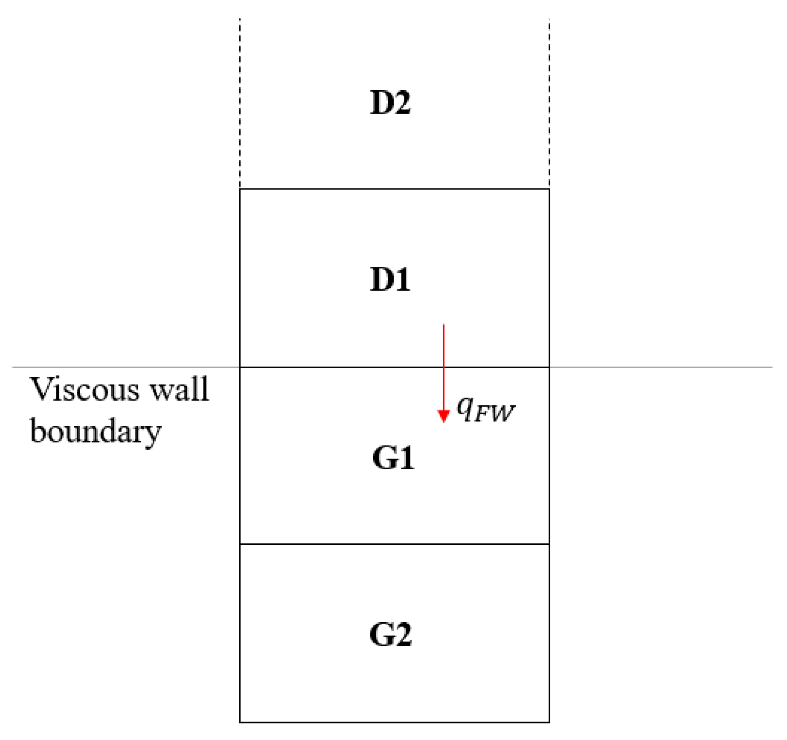
In order to establish the coupling with the solid domain, heat fluxes are imposed at the viscous wall boundaries adopting a thin shear layer approximation. The fluid mesh presents two layers of ghost cells in order to facilitate the computation of the fluxes at the interfaces [50]. The heat fluxes calculated in Equation (3) and processed through the DWI technique are associated with the corresponding fluid block boundaries in contact with the solid walls. With reference to Figure 5, D1 is the first layer of the inner fluid domain; G1 and G2 are the corresponding ghost layers. The fluid temperature in D1 is detected from the previous solver iteration, and the ghost cell temperature in the first layer is updated according to:
with as the distance between the cell centers and kfl as the locally computed fluid conductivity. Similarly, the temperature in the G2 layer is updated in cascade, with reference to the newly computed temperature in G1. The temperature values are used to calculate the corresponding cell densities considering a zero-order pressure extrapolation in wall normal direction, while the no-slip condition is assured by reversing the fluid tangential velocity components in the ghost layers. Equation (7) is linearized and accounted in the implicit scheme.

Figure 5.
Fluid domain discretization at block boundaries: D1 as the inner domain layer, G1-G2 as the ghost layers.
The rate of convergence induced by the Neumann boundary condition is influenced by the actual magnitude of the imposed heat flux in Equation (7). Since the hFFB method is employed in the present development, no under-relaxation factors are invoked for the update of the ghost cells temperatures, as they are replaced by the selection of a suitable virtual heat transfer coefficient , determinant for the stability of the coupling process [46].
2.5. Solid Mechanical Solver
Once the continuity of temperatures and heat flux is achieved at the interface of the two domains, an FEM linear elastic solver with quadratic elements presented in [51] is invoked for the solution of the von Mises stresses.
with as the stiffness matrix, referencing the vector of nodal displacements, and indicating the load.
Within the framework of the present analysis, the solid mechanical solver shares the same mesh as the heat transfer solver, as remarked in Section 3. Therefore, the previously computed nodal temperatures are directly assigned to the new linear system.
The right-hand side vector accounts for the centrifugal loading and the thermal strains, considering the effect of the material contractions and expansions induced by the temperature variations, which are computed as:
with α(Ti) indicating the temperature-dependent thermal expansion coefficient; Ti pointing to the node temperatures resulting from the CHT analysis; and Tref as the reference temperature at the initial state, at which no thermal stresses are present within the material [52]. In the current study, we refer to Tref as the ambient temperature. Through the thermal strains, the stresses in the material are dependent on the outcome of the CHT computation, which increases the complexity of the gradient calculation, as presented later on.
The maximum von Mises stress is computed using a p-norm function according to Equation (10), with p = 75.
Equation (10) fulfills the requirement of global differentiability, as it is a continuous function, and is invoked as a constraint within the optimization problem with the aim of keeping the thermo-mechanical stresses, induced through the Conjugate Heat Transfer, bounded to a prescribed value. The gradient of this constraint is computed by an adjoint methodology, as described in the next section.
3. Adjoint Solver
The structure of the primal solver evaluating the thermo-mechanical stresses is computationally expensive because the CHT procedure requires several loops of CFD-FEM analysis to reach the equilibrium of the temperatures and heat flux at the fluid–solid interface. For this reason, such a framework is less suited for gradient-free optimization methods, as a prohibitive large population of candidates would need to be evaluated using this expensive tool. A gradient-based optimization technique, on the other hand, may offer a faster convergence through a more guided search in the design space. Especially when combined with the adjoint method, the computation of the derivatives is very efficient and almost insensitive to the number of design parameters.
The evaluation of the cost function J in primal mode is a two-step process. The first one considers the values of the design variables and generates the correspondent geometry and finally the grid, whose points coordinates are expressed by the vector . The second step involves the flow solver and some post-processing routines, returning the value of J. Following the same approach in reverse mode, also the adjoint evaluation procedure is split in two parts: the first one computing the sensitivities of the cost function J w.r.t. the perturbations of the grid coordinates X, and the second one calculating the sensitivities of the grid coordinates X w.r.t the changes in the design variable α. Therefore, the CAD-based parametrization described in [21] allows transferring the grid sensitivities of the cost function to the design variables, controlling the component shape modifications by the application of the chain rule of differentiation expressed in Equation (11):
Within the thermo-mechanical analysis process developed in the present work, Equation (11) is invoked twice in order to account for the cost function sensitivities w.r.t. the coordinates of the fluid grid points and the solid grid nodes, respectively. Therefore, the global sensitivity expression can be decomposed as follows:
The remaining portion of this section is devoted to the calculation of the cost function sensitivities with respect to the fluid and solid grid coordinates, respectively and , operated through the application of a discrete adjoint method. Such sensitivities provide the descent direction for constrained or unconstrained multidisciplinary optimization problems with the aim of minimizing the thermally related response functions.
Consistently with the structure of the primal solver, the adjoint framework treating this interdisciplinary problem is formulated according to a “loose-coupling” approach, different from the “strong-coupling” techniques as described in [53]. In fact, the latter accounts for cross-discipline Jacobian terms implicitly exchanging boundary conditions between the fluid and solid domains, and therefore directly solving the global adjoint system at once. Instead, the selected partitioned-coupling method is less intrusive in the structure of the existing adjoint CFD solver from [19] and therefore more suited to a continuously growing modular multidisciplinary platform.
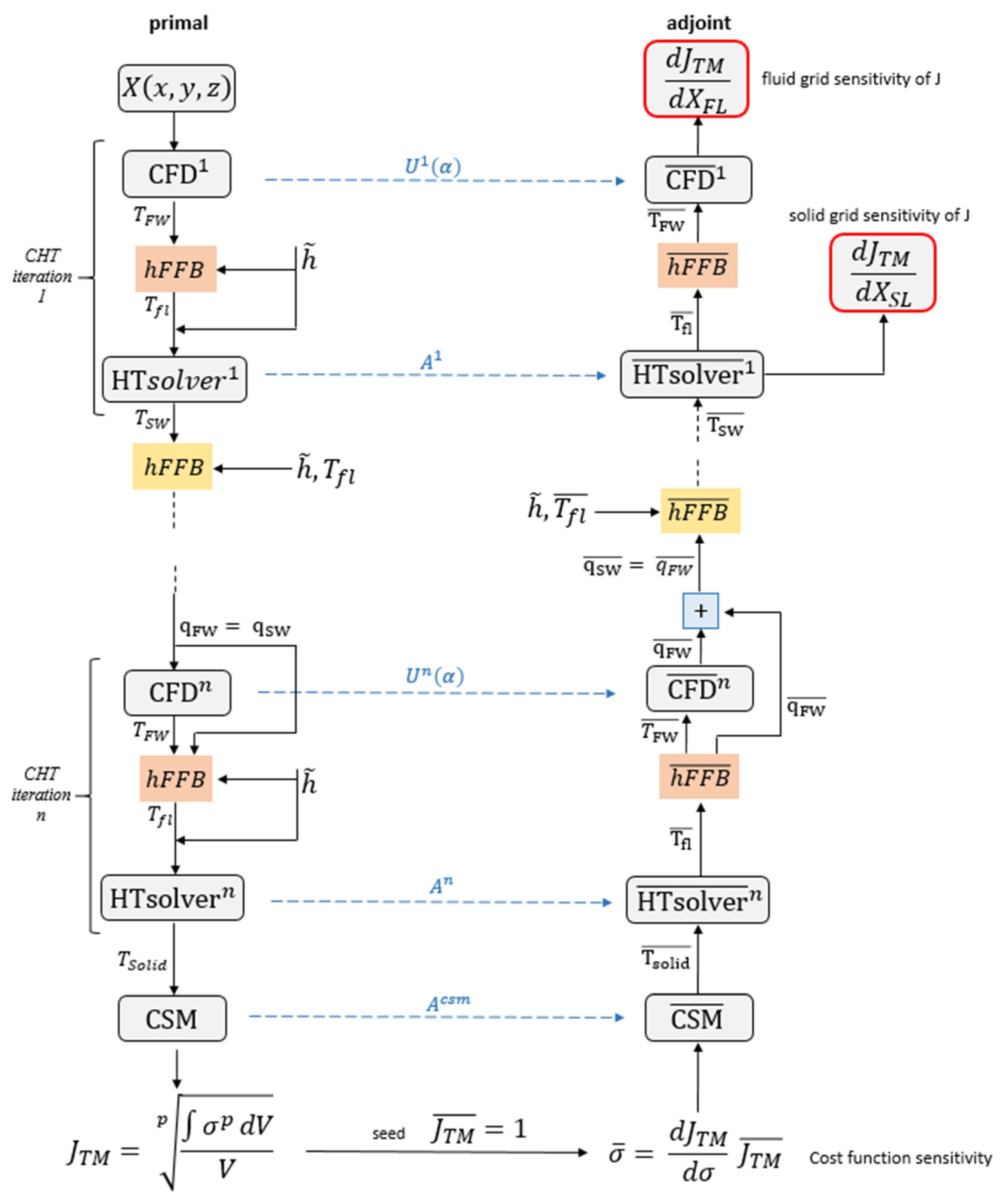
Figure 6 reports the framework of the thermo-mechanical evaluation, with the adjoint workflow on the RHS. The iterative structure characterizing the solution of the primal problem is maintained in its adjoint counterpart, which walks through the entire chain in reverse mode by the manual differentiation of the full process. Therefore, the adjoint branch is discussed starting from the bottom, till achieving the final grid sensitivities on the top.
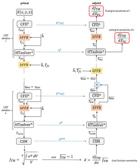
Figure 6.
Workflow for the primal and adjoint computations of steady-state thermo-mechanical constraints.
3.1. Adjoint Variables
The most demanding terms in the computation of Equation (12) are the sensitivities of the response function w.r.t. the grid coordinates. Since:
with u denoting the vector of the state variables, the application of the chain rule of differentiation results in the following decomposition:
Equation (14) holds for both the fluid and the solid grids. The second term at RHS presents the partial derivative of the cost function w.r.t. the state variables . Since the current problem exhibits a multidisciplinary footprint, the hierarchical structure of the workflow in Figure 6 implies that the output states contributing to the p-norm calculation in Equation (10) depend on the intermediate ones evaluated by the preceding CFD and FEM solvers. Therefore, according to the principle of the “reverse differentiation” [54] we choose for instance an output variable , whose sensitivity is known, and calculate its sensitivities w.r.t. each intermediate state till the initial one, such that:
Since the work focuses on the single thermo-mechanical output expressed by Equation (10), herein named y, we can associate with any intermediate state variable a new variable , called the adjoint variable, defined as:
The upper bar notation follows the convention for adjoint variables reported in [54].
Hence, we apply the chain rule walking throughout the original trace in Figure 6 in backward mode, paying attention to the opposite propagation of the adjoint variables with respect to the physical ones. This technique finally returns the sensitivities of the response function w.r.t. the initial state variables.
The following sections describe the backward propagation process in detail, with the aim of offering a guidance to the development of the adjoint method.
3.2. Adjoint Response Function
The adjoint framework is initiated by seeding the maximum von Mises constraint. Since , the input is:
The maximum von Mises stress is function of the components of the Cauchy stress tensor. Therefore, in reverse mode the adjoint stress components are calculated as:
On the other hand, Equation (10) shows an explicit dependence over the solid grid coordinates through the two volume integrals appearing at the numerator and denominator. Therefore, the constraint function sensitivities with respect to the solid grid coordinates are accumulated as follows:
In Equation (19), the operator “+=” is reported to emphasize the concept of accumulation of the sensitivities w.r.t. the solid grid coordinates that is propagated backwards throughout the adjoint workflow till the grid generation procedure. Moreover, the notation is adopted for the sake of simplicity, while in reality the sensitivities over the three dimensions (X,Y,Z) are accounted in the development.
Finally, in the remaining portion of the document the notations and will be skipped in favor of the more convenient and .
3.3. Adjoint Mechanical Solver
The evaluations through the mechanical solver involve the multi-step approach outlined in Figure 7, where the primal mode is represented along with its adjoint counterpart. Notably, the reverse computation follows the backward propagation of the adjoint variables, closely resembling the primal scheme. The related procedure is discussed in detail in this section.

Figure 7.
Evaluation by mechanical solver: primal and adjoint modes.
In primal mode, the stress components are computed from the elasticity matrix of the material under consideration and the strain components. Thus, the differentiation in reverse mode returns the adjoint strains .
Here, the adjoint stresses are the once computed by the reverse differentiation discussed in Section 3.2.
The adjoint mechanical strains and the adjoint thermal strains appear in Equation (20). Since the thermal strains exhibit direct dependence from the nodal temperatures through the term and indirect dependence through the thermal expansion coefficient α(T), the relative contributions to the adjoint solid node temperatures are accumulated and propagated to the next step in the reverse workflow.
Additionally, also the elasticity matrix E depends on the nodal temperature, which leads similarly to contributions for the adjoint solid node temperatures.
The process of accumulation of the contributes to the adjoint temperatures field is facilitated by the commonality of the solid grid coordinates between the mechanical and heat transfer solvers, as no re-interpolations are necessary for the backward propagation of the sensitivities.
Next, recalling that the mechanical strains in primal mode are calculated from the vector of nodal displacements u, the adjoint nodal displacements are derived by the reverse differentiation () and provided in input to the adjoint mechanical solver.
The iterative linear system solver adopted in primal mode for the solution of Equation (8) is not directly differentiated but, as discussed in [20], a new linear system is formulated with the adjoint displacements vector appearing at RHS as:
The system (23) is solved for the adjoint load vector , while the transpose of the stiffness matrix S, previously computed in primal mode, appears at LHS. Therefore, the adjoint stiffness matrix is obtained from the system (24).
Finally, the system assembly process is algorithmically differentiated, returning the grid sensitivity accumulation:
The system (25) accumulates the grid sensitivities attributed to the mechanical solver. The adjoint temperatures deriving from Equations (21) and (22) are provided as input to the adjoint heat transfer solver at the next section, thus linking the structural solver to the iterative adjoint CHT process.
3.4. Adjoint Heat Transfer Solver
Consistently with the previous section, the iterative linear system solver adopted in primal mode for the solution of Equation (6) is not directly differentiated, whilst the adjoint load vector and the adjoint stiffness matrix are computed through the new linear systems in Equation (26).
Equation (26a) shows the transposed stiffness matrix accounting for the conductive and convective terms previously calculated in primal mode, while the adjoint temperature vector from Section 3.3 is imposed at the RHS. The resulting adjoint load vector is assigned to Equation (26b), together with the temperature solution stored at the last CHT loop in primal mode, contributing to the calculation of the adjoint stiffness matrix .
Similarly to Equation (25), the system assembly process is algorithmically differentiated and the adjoint contributes to the solid grid coordinates are accumulated. Since the thermal solver and the mechanical solver share the same grid, a unique vector of solid grid sensitivities is accumulated and propagated backwards throughout the CHT workflow.
The convective loading at the RHS of the system (6) accounts for the virtual bulk fluid temperature. Its adjoint counterpart is computed from (returned by Equation (26a)) and from the user-defined virtual heat transfer coefficient .
is not accumulated along the entire adjoint workflow but recomputed at every CHT loop in reverse mode and then passed to the adjoint hFFB routine.
3.5. Adjoint hFFB Procedure (Solid → Fluid)
The adjoint virtual bulk fluid temperature field associated with the solid nodes is processed by algorithmic differentiation, returning the adjoint assigned to the neighboring fluid cells centers. Equation (28) reports the DWI procedure in primal mode on the left, with focus on the calculation of the solid temperature at node j, leveraging the information of the cluster of i = (1, ..., n) neighboring fluid cells. On the right, the backward differentiation of the interpolation procedure results in the adjoint temperature field associated to the fluid domain. The operator “+=” stresses the fact each fluid cell may belong to the “neighboring cluster” of different solid nodes j, and therefore would accumulate their adjoint values.
Equation (28) suggests also that additional contributions to the solid grid sensitivities and to the fluid grid sensitivities can be accumulated through the adjoint vector of mapped distances between each solid node and the corresponding fluid neighbors, , as detailed in Section 2.1. Thus, after deriving the adjoint distances as , the cells-nodes mapping routine is differentiated and the contributions to the two grids are obtained.
Finally, the algorithmic differentiation of Equation (1) returns the adjoint temperature at the fluid walls , which is used as input to the adjoint CFD solver at the next step, and the adjoint wall heat flux , stored for a later accumulation.
3.6. Adjoint Fluid Solver
The partitioned coupling technique adopted in this work allows for non-intrusive calls to the in-house adjoint CFD solver. The flow field is initialized with the converged flow solution U from the corresponding CHT loop in primal mode, and the viscous wall temperatures in the ghost cells layers are updated again imposing the Neumann boundary condition, as reported in Equation (7).
The adjoint fluid wall temperature , resulting from the reverse hFFB procedure at the previous step, contributes to the linearization of the constraint function with respect to the conservative flow variables U and the fluid grid coordinates . The adjoint equation discussed in [19] is repeated here for convenience:
with R as the non-linear residuals of the primal flow solver, ψ indicating the unknown adjoint variables, and J the objective or constraint function of interest. Therefore, the RHS term linearized at the viscous walls exposed to the heat flux from the solid develops by the chain rule as follows:
with Vbnd as the primitive variables computed at the boundary of interest, Vdomain as the corresponding variables from the interior of the fluid domain, and the last term indicating the transformation matrix from primitive to conservative variables.
Similarly, the linearization of the cost function w.r.t. the fluid grid coordinates is the following:
Therefore, the first term at RHS linearized at the viscous walls with heat flux results in:
Equations (31) and (33) show the contributions of the adjoint fluid wall temperatures calculated in Section 3.5 to the fluid grid sensitivities at the wall boundaries exposed to the heat flux.
For the principle of the reverse accumulation, the wall heat flux term, entering in primal mode as the update of the boundary conditions in Equation (7), results in an adjoint fluid wall heat flux that is computed once the adjoint CFD solver approaches full convergence. This contribution is summed up with the returned in Section 3.5 by the reversed hFFB procedure.
A further contribution derives also from the second layer of ghost cells, not reported in Equation (34) for the sake of simplicity.
3.7. Adjoint hFFB Procedure (Fluid → Solid)
The partitioned coupling scheme in reverse mode completes by transferring the adjoint terms from the fluid to the solid domain. is processed by the differentiated DWI procedure, similarly to Equation (28), and returns the adjoint heat flux associated with the solid grid nodes. Consistently with the previous call, additional contributions are accumulated to the solid grid sensitivities and to the fluid grid sensitivities through the adjoint vector of mapped distances between each fluid cell center and the neighboring solid nodes.
Finally, the routine adopted to calculate the wall heat flux within the solid domain in Equation (3) is algorithmically differentiated, accounting only for the nodes laying on the interface. This process results in the new field of adjoint solid temperatures , passed to the adjoint heat transfer solver described in Section 3.4.
The whole adjoint CHT process is iteratively repeated from Section 3.4, Section 3.5, Section 3.6 and Section 3.7 for as many loops as the ones performed during the primal computation till convergence.
Once walked through the entire workflow in reverse mode, and , enclosing the contributions from the entire multidisciplinary chain, are introduced in Equation (12), and the constraint function sensitivities w.r.t. the design variables are finally computed. Hence, is evaluated by the SQP-based optimizer and the geometry is updated, opening the path to a new thermo-mechanical evaluation within the history of the shape optimization problem.
4. Validation
4.1. Flat Plate (Primal Mode)
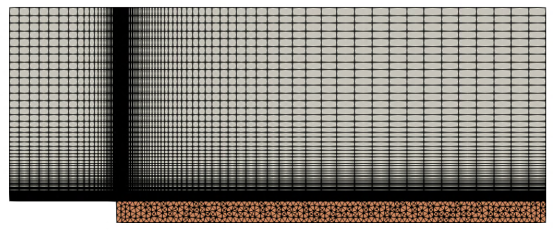
The validation of the CHT process in primal mode is performed with the consideration of the analytic solution offered by [33] for the conjugate problem applied to a flat plate subjected to an incompressible flow. The mesh characteristics and boundary conditions are reported in Table 1, while the fluid and solid meshes are qualitatively shown in Figure 8. The thermal conductivity adopted for the solid phase is aimed at obtaining an average Biot number around unity.

Table 1.
Flat plate domain characteristics and boundary conditions.
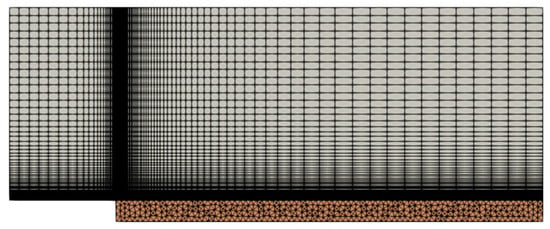
Figure 8.
Fluid and solid meshes for the conjugate problem applied to a flat plate.
The convergence history of the maximum temperature difference between two successive fluid–solid iterations is reported in Figure 9, where a threshold of 1K is selected as the stabilization criterion for the model.
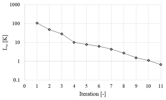
Figure 9.
Convergence history of L∞.
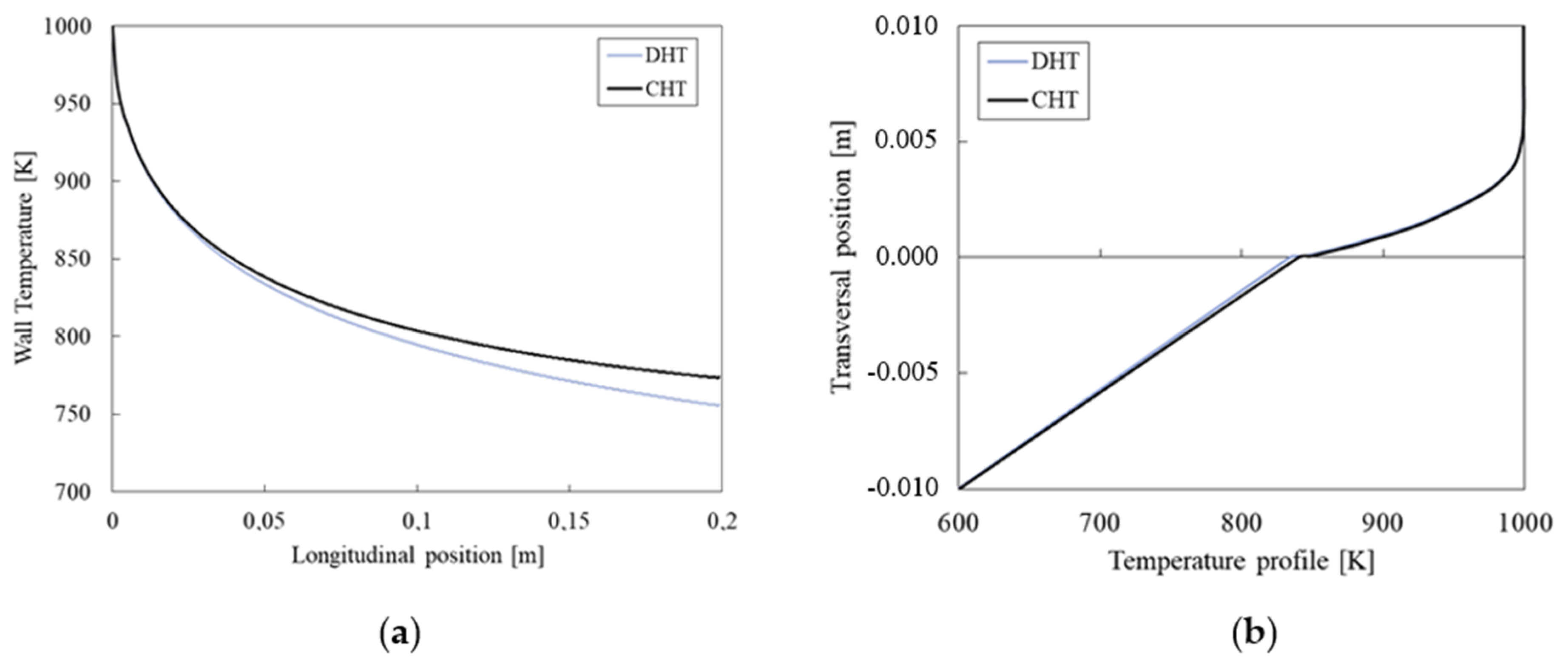
The distribution of temperature at the interface between the two domains is presented in Figure 10a, comparing Luikov’s differential heat transfer (DHT) solution with the numerical one. Figure 10b shows the temperature variation in a vertical section located at x = 0.05m. In both cases, a sufficient agreement between the numerical results and the analytic solution is obtained within the limitations of the DHT approach, which does not capture the effect of the solid conductivity in the streamwise direction, as explained in [55].
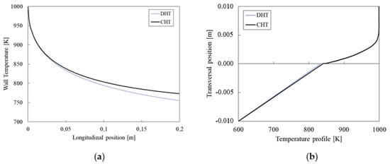
Figure 10.
CHT problem for flat plate: (a) temperature at the domain interface, (b) temperature profile at x = 0.05 m. Numerical vs. analytic solution.
4.2. Rotor Mesh Sensitivity Analysis
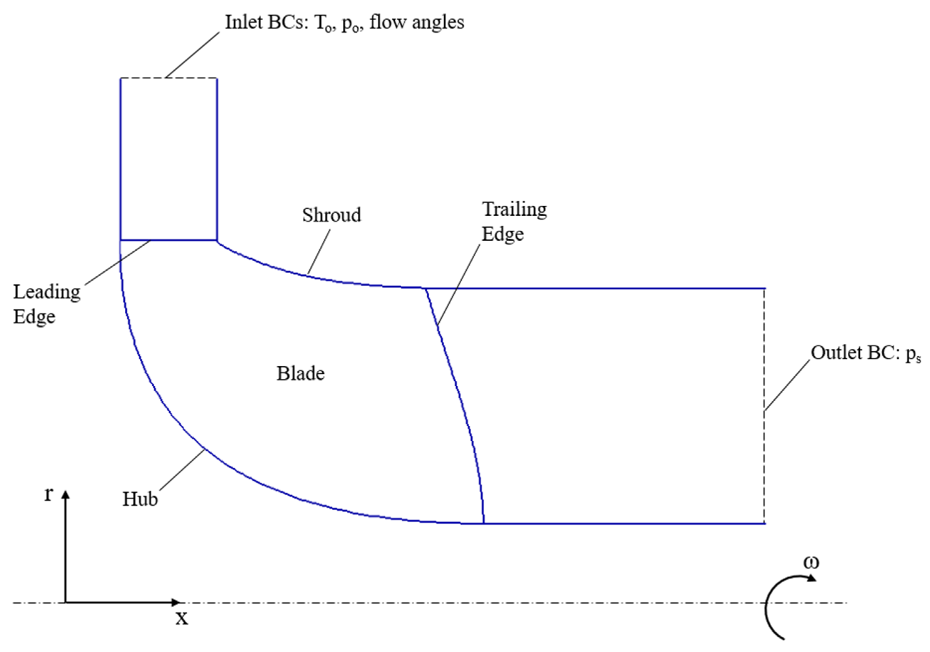
A mesh sensitivity study for the CHT analysis is performed on a three-dimensional test case presented in [19], considering a radial turbine impeller with 10 blades and an inlet diameter of 50 mm. A two-dimensional sketch of the domain on the meridional plane of the rotor is reported in Figure 11, along with the locations of the imposed boundary conditions. The method of the characteristics [56] is adopted to establish the number of physical conditions to be assigned at the inflow and outflow boundaries. The total upstream temperature and pressure are specified at the inlet of the domain, along with flow velocity components in the corresponding coordinate system. At the subsonic outflow boundary, a single flow variable is imposed, specifically the downstream static pressure. In conclusion, the boundary conditions applied to the problem are summarized in Table 2, in which the impeller rotational speed is also included.
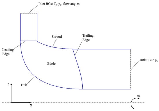
Figure 11.
Turbine rotor meridional view and boundary condition locations.

Table 2.
Turbine rotor boundary conditions.
The interactions of the rotor fluid and solid meshes are explored over three levels of refinement, as summarized in Table 3. Additionally, three values of the virtual heat transfer coefficient are investigated in order to determine a suitable trade-off between stability and computational time. These factors are explored following the combinations expressed by the L9 Orthogonal Array method [57], returning nine test cases (Table 4).

Table 3.
Fluid and solid mesh refinements, levels.

Table 4.
L9 Orthogonal Array applied to the turbine rotor CHT analysis.
All the simulations are run till convergence at a relative residual drop of 10−8 for the computational fluid dynamics (CFD) solver and 10−10 for the FEM solver, while the CHT workflow is stopped for a maximum deviation in wall temperature between two successive fluid-solid iterations L∞ below 1 K. y+ values below unity are obtained for the “mid” and “fine” levels of the fluid grid refinement, while the coarsest one exhibits a peak in y+ around 2.5 at the blade leading edge. Concerning the maximum number of nodes in the solid mesh, the code was tested up to the finest possible grid before incurring in memory leakage issues with the adopted Conjugate Gradient iterative solver.
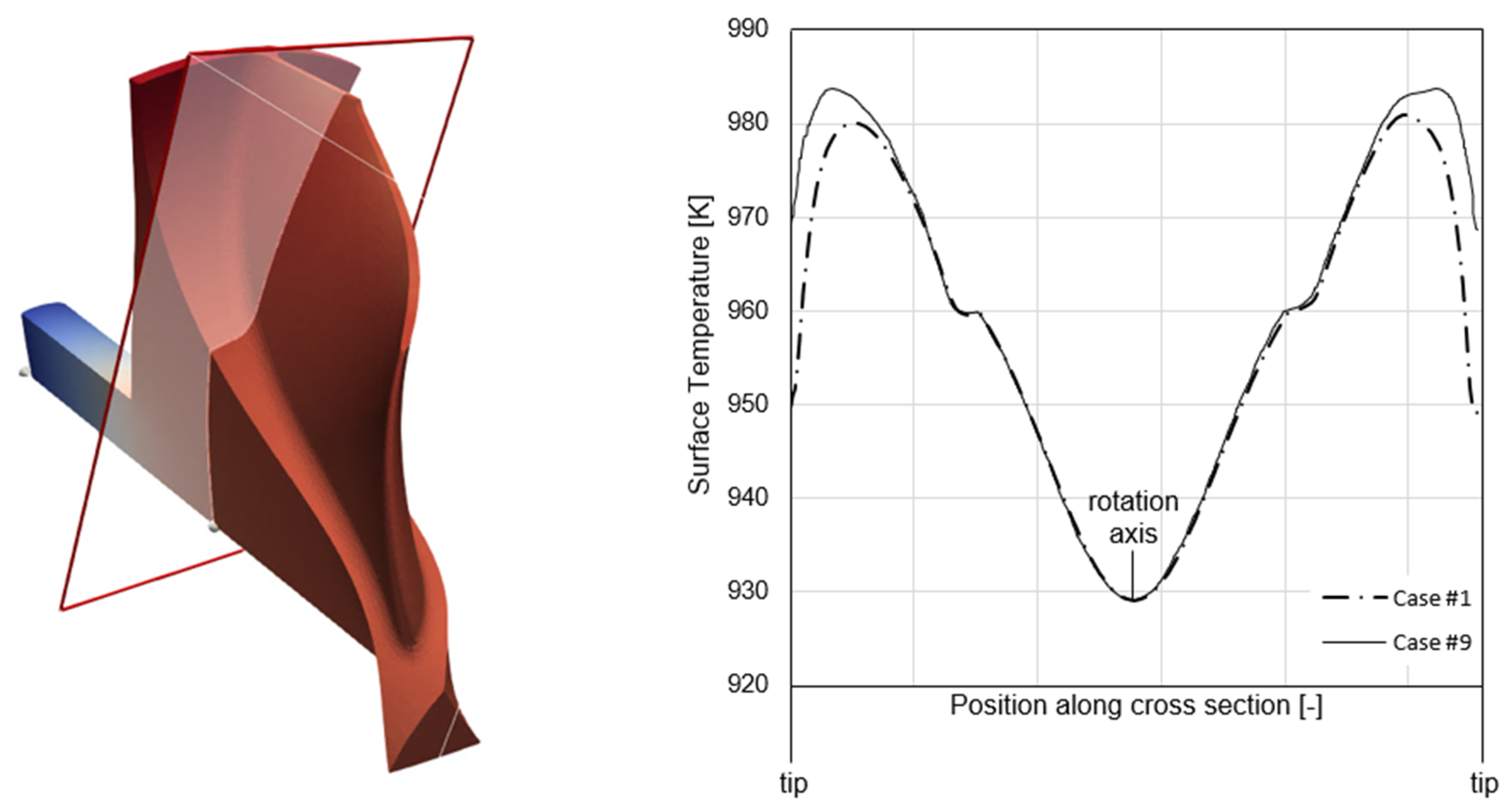
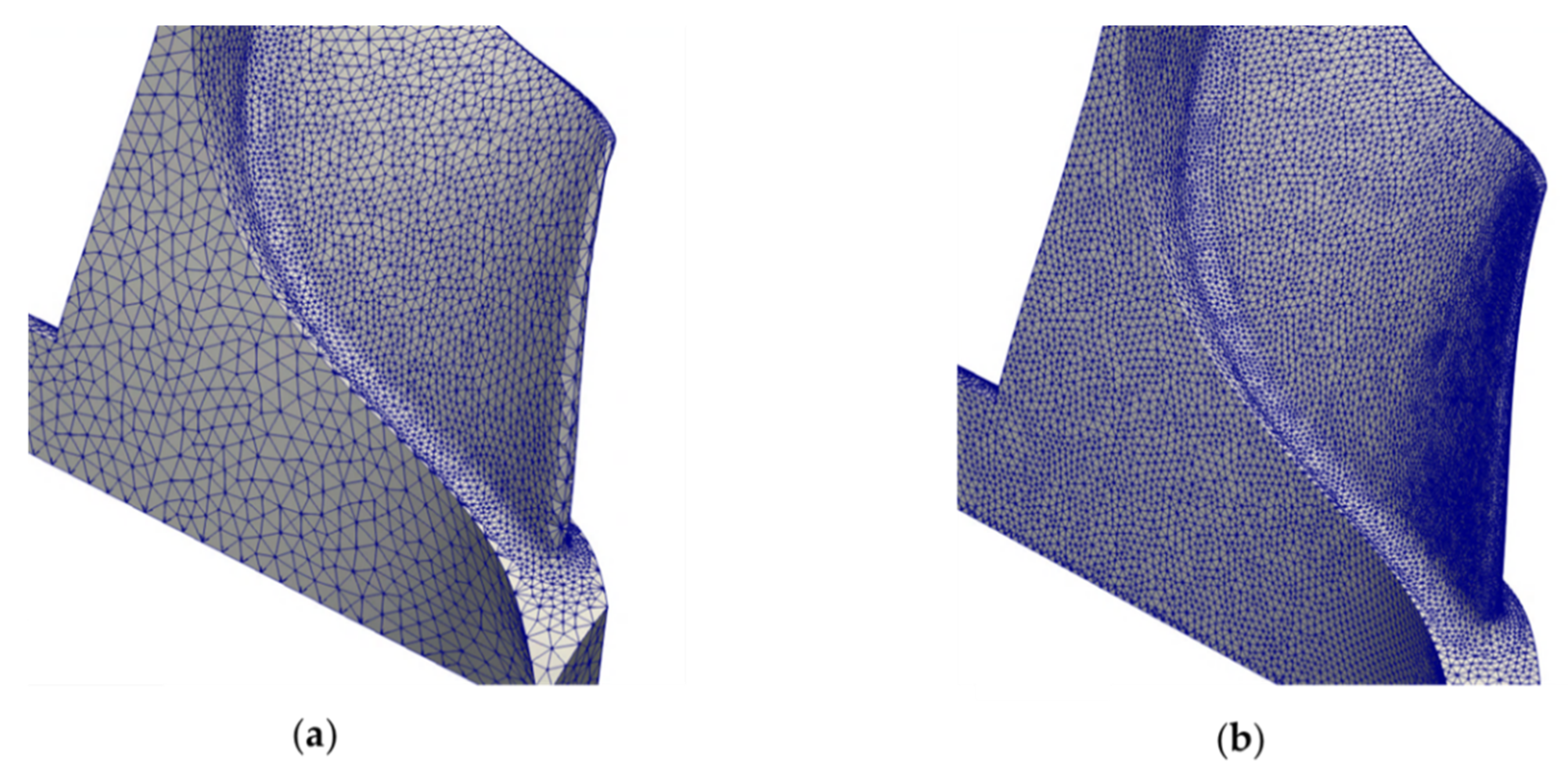
The results in Table 5 demonstrate a low sensitivity of the maximum temperature in the solid domain due to the settings applied to the coupling process, except for the first test case with coarse meshes at both the fluid and solid side. A critical aspect is represented by the quality of the interpolation of the information between the two domains realized by the fine-tuned distribution of virtual grid points on the interface at fluid side, as discussed in Section 2.1. Moreover, the finest solid mesh increases the resolution of the convective loading, resulting in more accurate temperature predictions in the material and, therefore, also more reliable heat fluxes returned to the fluid. Figure 14 shows two cases of solid mesh size, the coarse one (Figure 14a) and the intermediate one (Figure 14b), with the addition of the trailing edge refinement described hereafter. In the case of finer solid grids, the interpolation procedure returns a richer temperature pattern at the interface, closely mirroring the fluid conditions at the walls, whilst the coarsest one approximates the thermal loading distribution with the highest deviations localized in the blade tip region, where large secondary flows and leakages are present, and at the trailing edge. In this respect, a surface temperature analysis at a cross section located at about 25% of the chord was performed in order to evaluate the integral of the temperature deviations between each investigated test case w.r.t. test case 9. The axial position of the planar section was chosen in a region of high convective perturbations due to the presence of a significant flow detachment at the blade leading edge. The results, summarized in Table 5, are supported by the example in Figure 12, showing the temperature contours for case 1 and case 9. It is interesting to note that, in both set-ups, the blade tip returns significant thermal gradients because of the thinner geometry exposed to the flow vortices. However, the coarsest mesh overestimates the temperature drop, resulting in the integral reported in Table 5.

Table 5.
Fluid–solid grid sensitivity: summary of CHT computations.

Figure 12.
Temperature contours for test case 1 and test case 9 at the planar cross section on the blade.
Finally, considerations about the computational time are synthesized in Table 5, with a dominant portion covered by the CFD solver and a significant rise in overhead emerging from the FEM heat transfer computations at the finest grid level. The normalization refers to the total duration of a single CHT iteration, including also the hFFB procedure. The comparison is performed w.r.t. the reference duration of test case 1, presenting the coarsest meshes at both fluid and solid side.
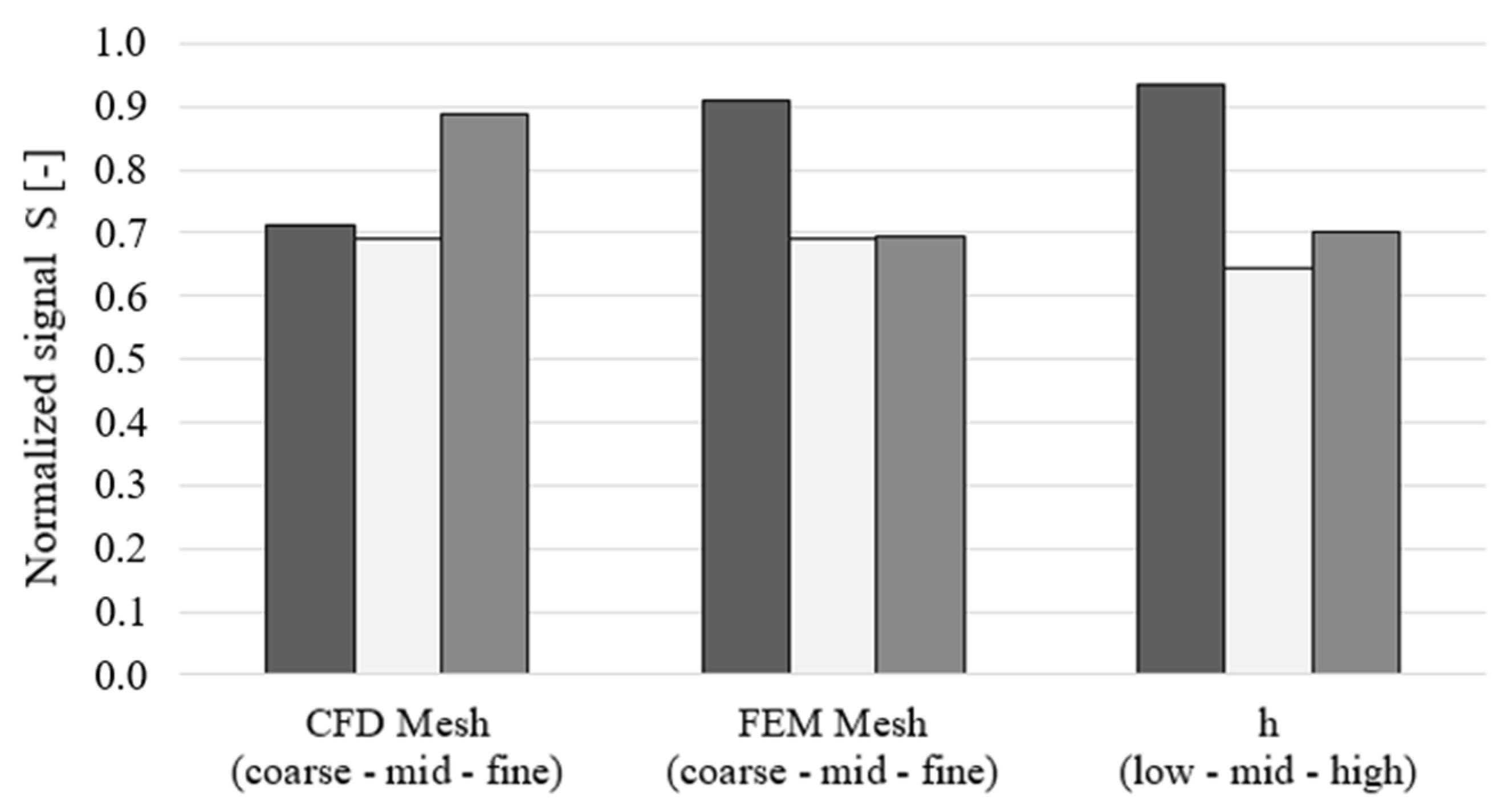
The interactions among the three factors in the Orthogonal Array from Table 4 are studied through the compounded signal S, defined as:
with the term A enclosing the normalized difference between the maximum temperature predicted by the test case of interest and test case 9 (showing the finest grids), B representing the normalized computational time, and ω as the weighting coefficient. In the current study, ω = 0.7 in order to bias the objective function towards the accuracy of the coupling process. Indeed, the factors levels finally expected from this study are the ones minimizing the signal S.
The analysis of the Orthogonal Array [57], resulting in Figure 13, reveals the dependence of the signal S from the three variables and their correspondent levels. The chart illustrates the virtual heat transfer coefficient is selected at its highest value within the stability region of the Biot number discussed in [46], as it influences the B term in Equation (36), determining the rate of convergence of the CHT coupling process. Indeed, the current problem exhibits an optimal = 1000 W/m2 K, since the highest value approaches the limit of the stability region, with incipient oscillations in the value of heat flux exchanged at the interface, before reaching convergence. The solid grid size, instead, characterizes the accuracy of the interpolation of the quantities passed between the two domains through the DWI process and affects the A term in Equation (36). In general, finer solid grids are favored by the current analysis. Remarkably, the fluid mesh size follows an opposite trend because its influence on the A term is less pronounced, as the coarsest level already provides good-quality solutions. On the other hand, the signal S is driven by the increase in computational overhead experienced with the fluid mesh refinement.
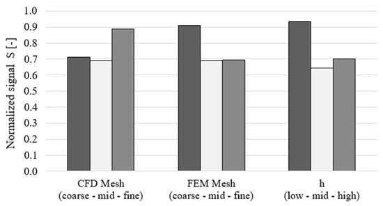
Figure 13.
Normalized signal S dependence from factor levels in the Orthogonal Array.
Since the weighting coefficient ω privileges the accuracy of the CHT coupling process, the final selection of the factors levels results in the intermediate values for the refinements of both the grids and for the virtual heat transfer coefficient. However, it is recognized that smaller solid element sizes improve the stability of the CHT coupling process because it avoids local poor quality in the discretization of the blade surface in correspondence with thin regions (Figure 14a), potentially inducing drops in the local Biot number and inconsistencies with the selected value from a stability standpoint. Therefore, the issue is addressed by the generation of a “hybrid” configuration (Figure 14b), envisaging a local solid mesh refinement in correspondence with the blade tip surface and trailing edge, whilst maintaining the intermediate element size in the rest of the domain. This last setup increases the mesh density to a total node count of about 420 k.
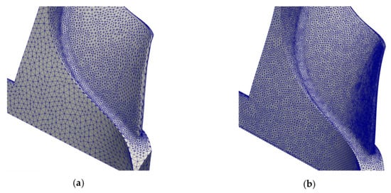
Figure 14.
Comparison of solid mesh refinements: (a) coarse grid, (b) hybrid-mid grid.
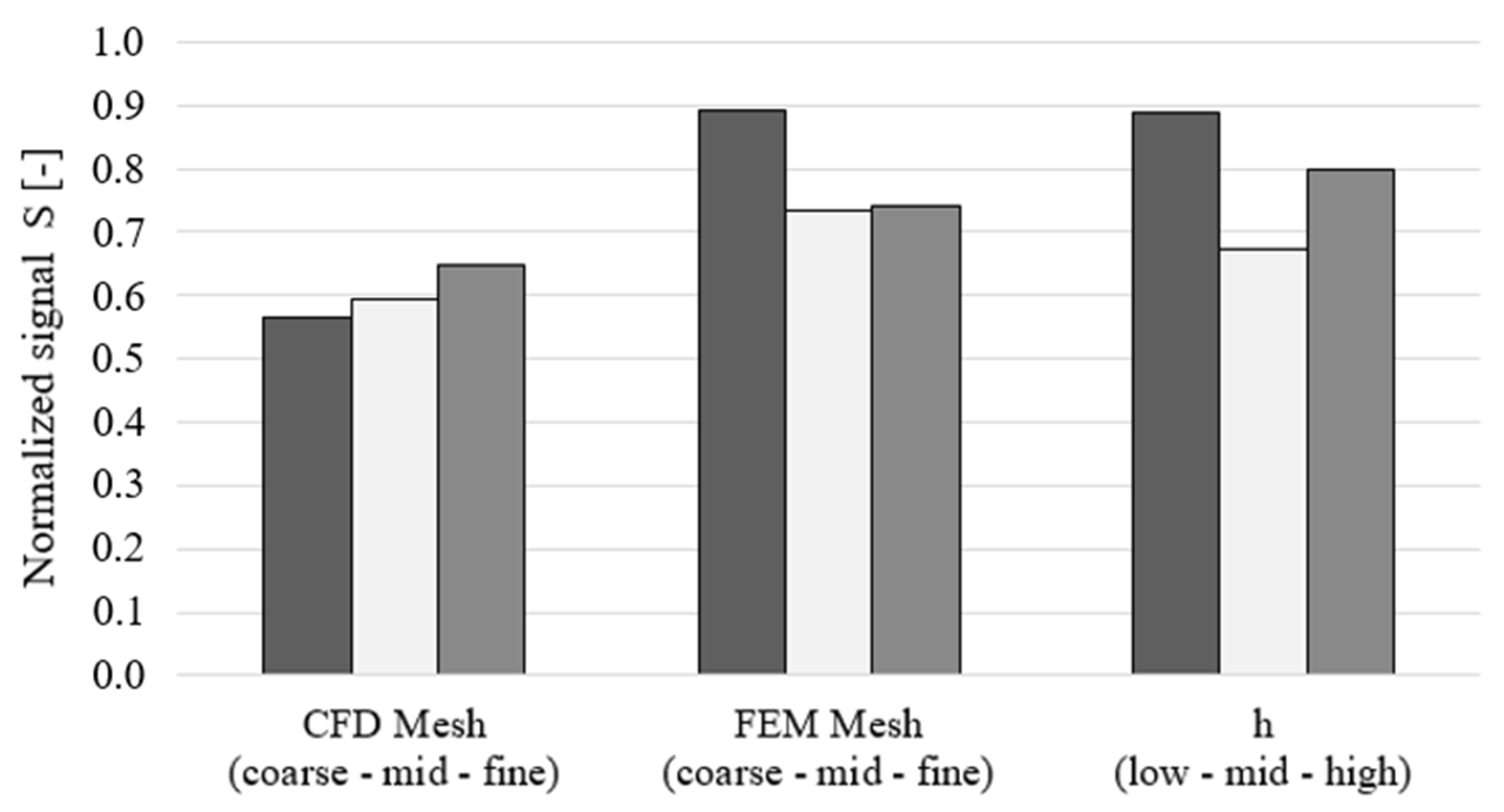
Finally, the Orthogonal Array analysis is repeated, assigning the integral of temperature deviations to the A term in Equation (36). The outcome, shown in Figure 15, confirms the previous considerations, except for the fluid mesh size, which promotes the trend towards the coarsest mesh because it still provides sufficiently accurate results. However, since the difference between the coarse and intermediate meshes is moderate, the previous selection of the medium size grid will be pursued for the sake of improved prediction accuracy.
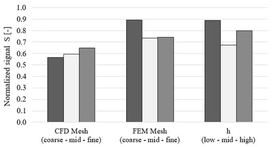
Figure 15.
Normalized signal S dependence from factor levels in Orthogonal Array—integral of temperate deviation assigned to term A.
Based on such considerations, the settings returned by the analysis of the Orthogonal Array are considered for the further assessments of the coupling problem.
4.3. Gradients Accuracy Evaluation
The present work accounts for the manual differentiation of the multidisciplinary process shown in Figure 6. The sensitivities are accurately computed by the reverse Algorithmic Differentiation technique [54] for what concerns the FEM solvers and the hFFB process, while the partitioned coupling approach opens the path to the direct integration of the in-house adjoint CFD solver.
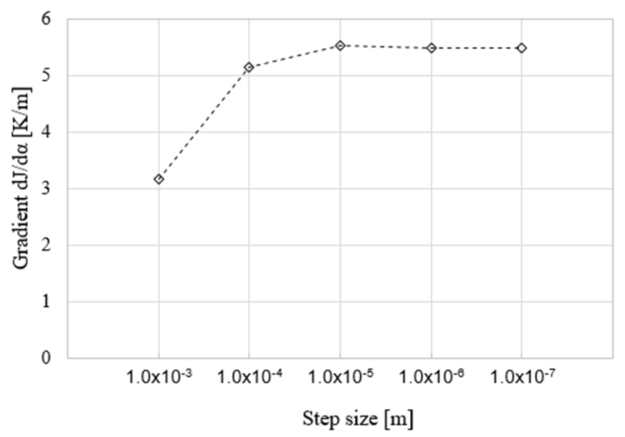
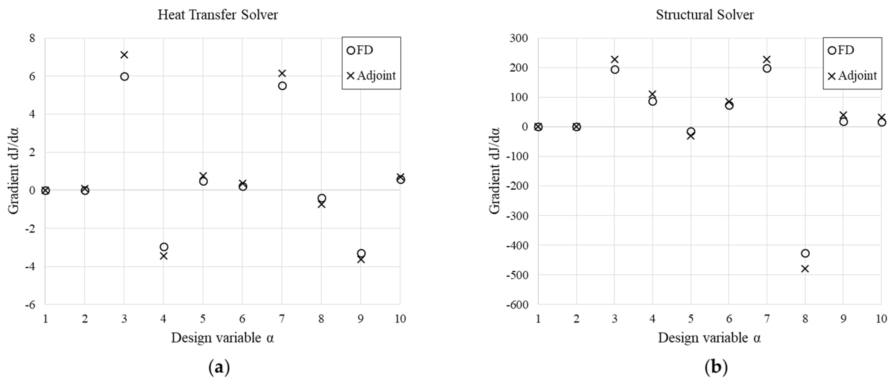
The validation of the differentiated FEM solvers is presented herein with reference to the rotor test case from Section 4.2. The adjoint sensitivities of the maximum temperature and of the maximum von Mises stress including the thermal strain w.r.t. selected design parameters (referenced in Table 6 and Figure 16) are compared to the correspondent gradients computed by the Finite Differences (FD) technique. The latter accounts for evaluations by a central differencing scheme, whose optimal step size is searched with the aim of accurate gradients computations. An exemplary case is reported in Figure 17, showing the identification of a suitable step size at the value of 10−6 m for the seventh design variable in the framework of thermal evaluations by the heat transfer solver. The magnitude of the perturbation must avoid too-small values, resulting in round-off errors, and too large values as well, because they introduce significant truncation errors. This outcome results from the evaluation of the cost function at each step size by solving the linear system obtained after the perturbation of the mesh through the morphing technique described in [20].

Table 6.
Design variables adopted in the dJ/dα gradient validation.
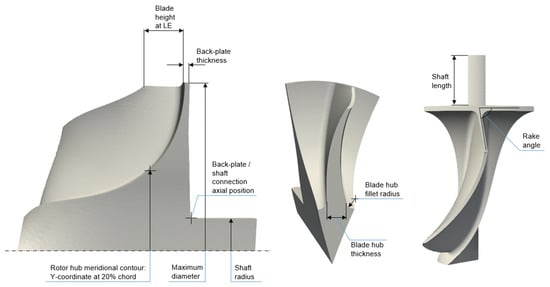
Figure 16.
Design variables from Table 2.
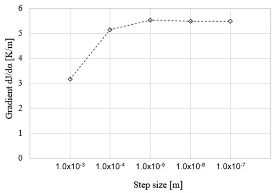
Figure 17.
Step size evaluation for the computation of dJ/dα by Finite Differences: Heat Transfer solver, variable 7.
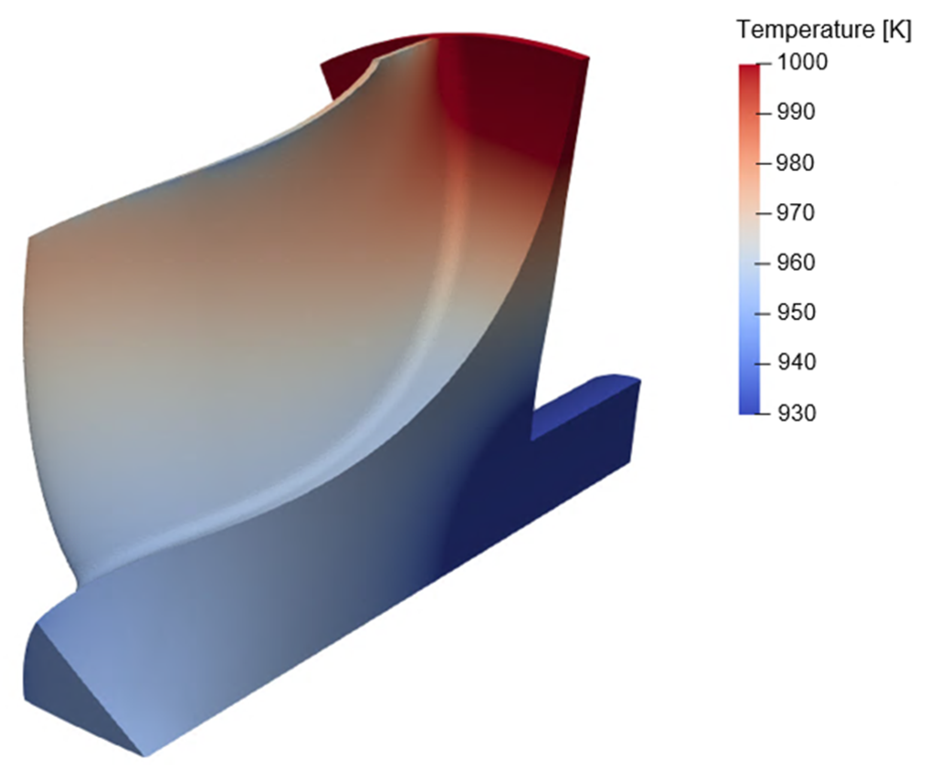
The sensitivities of the maximum solid temperature to perturbations of the ten design variables are summarized in Figure 18a, which shows a close agreement between the two methods, both in sign and magnitude. To understand the sensitivity analysis in detail, let us consider the thermal paths in the turbine rotor experiencing the convective loading resulting from the operative condition reported in Table 2, along with a convective condition on the back-plate surface with a uniform fluid temperature of 950 K and a Dirichlet boundary condition of 500 K assigned to the extreme section of the shaft.
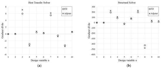
Figure 18.
Comparison of the dJ/dα sensitivities of the solid maximum temperature (a) and the maximum von Mises stress (b): gradients computed by the adjoint method vs. Finite Differences.
Figure 19 reveals that the maximum temperature is detected at the nodes in the region of the hub, in proximity with the leading edge. The computation of such constraint through a p-norm function returns a marked sensitivity from the rotor back-plate thickness, whose enlargement would reduce the influence of the heat sink located at the back-plate outer surface. Similarly, an increase in blade height at the leading edge would extend the thermal path to the colder areas highlighted at the tip, while an elongation of the shaft itself would reduce the gradient field. On the contrary, an increase in the turbine shaft diameter, an advancement of the axial position of the intersection between the rotor back-plate and the shaft, and an enlargement of the blade hub thickness would favor the cooling of the hub upper region. Such sensitivities provide the descent direction for a constrained optimization problem aimed at limiting the maximum rotor temperature for the sake of extended lifetime.

Figure 19.
Solid temperature on turbine rotor (operative condition from Table 2).
Similarly, the accuracy of the adjoint structural solver sensitivities is assessed by comparison with the same gradients computed by Finite Differences. The results reported in Figure 18b confirm the suitability of the manually differentiated framework.
Moreover, the time for the computation of the adjoint-based gradients for the heat transfer solver and the structural solver was measured. If X is the time required for the computation of the multidisciplinary workflow in primal mode and the problem accounts for n design variables, the calculation of the gradients by Finite Differences would approximately cost n ∙ X. On the contrary, the application of the adjoint method herein described costs about 8.6X for the heat transfer module and 2.3X for the structural analysis, in fair agreement with the original expectations. Such costs mostly depend on the assembly process of the differentiated system (Equation (25)) rather than the solver itself.
Finally, the loose-coupling approach adopted for the development of the CHT workflow allows the direct integration of the in-house adjoint CFD solver, and the accuracy of the computed gradients was already demonstrated by the same author.
5. Results and Discussion
The design work aims at reducing the thermo-mechanical stresses in the turbine impeller presented in Section 4.2. The operative condition in Table 2 is considered, along with a Dirichlet boundary condition with a temperature of 500 K imposed at the extreme cross section of the shaft, emulating the heat sink provided by the oil cooling circuit in the turbocharger bearing housing. The contribution of the thermal strains introduced by the present work improves the accuracy of the computation of the von Mises stresses, whose gradients provide information for the geometry modifications.
According to the grids selection anticipated in Section 4.2, the fluid domain is discretized with a multi-block structured mesh of about 1.3 M cells with boundary layer refinement. The solid domain accounts for an unstructured grid of approximately 420 k nodes and second-order tetrahedral elements.
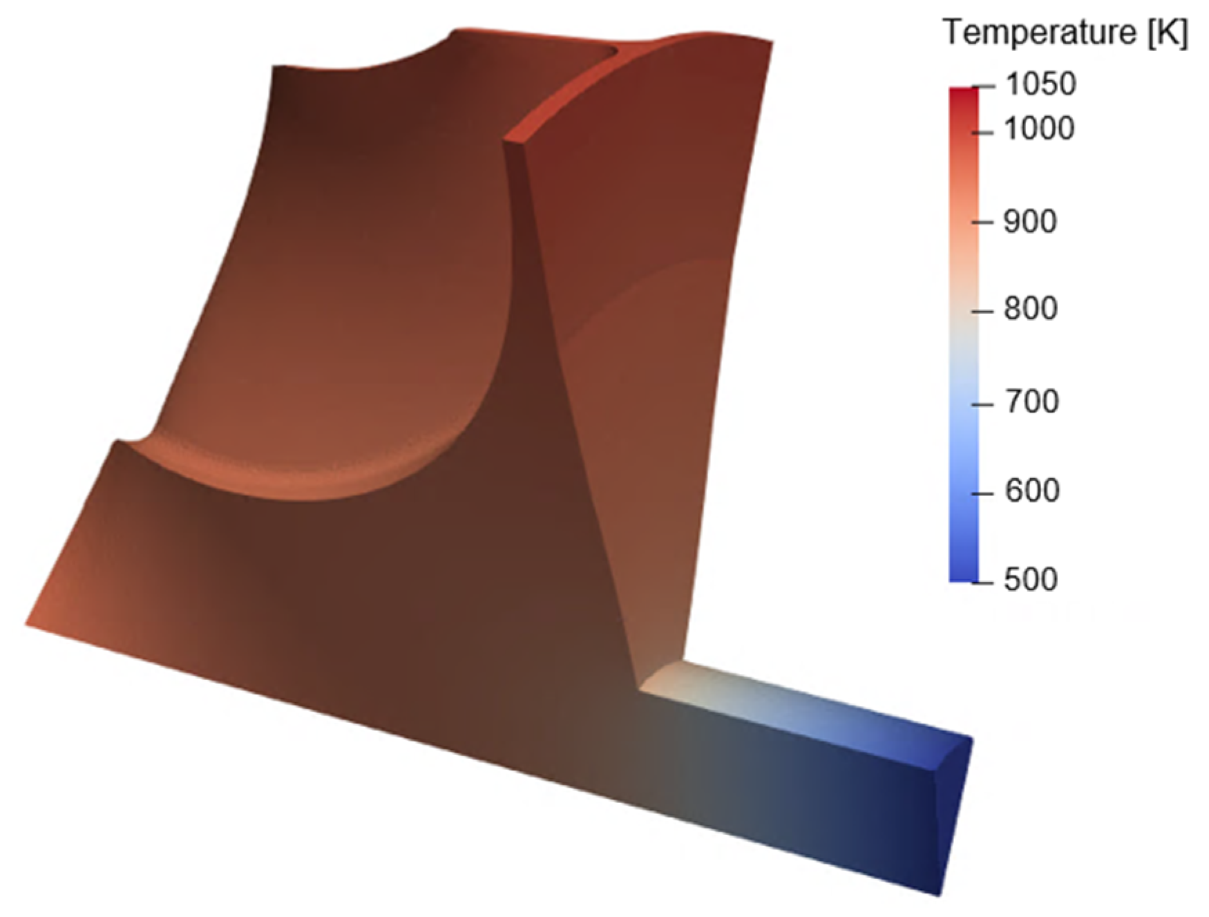
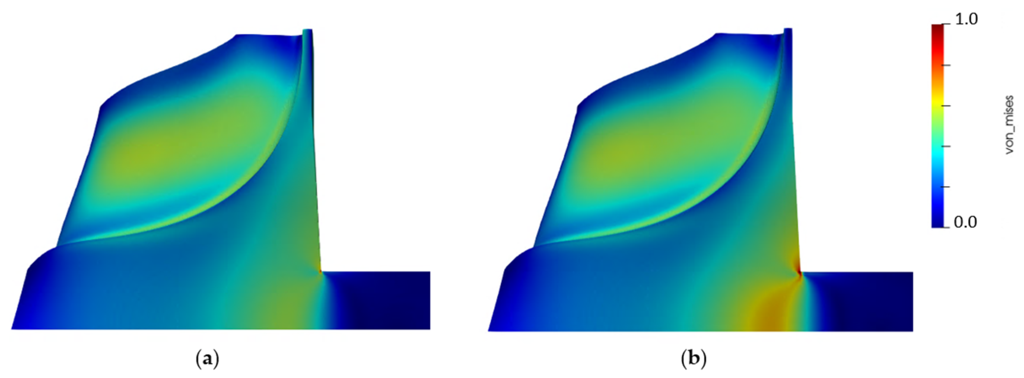
Figure 20 presents the temperature distribution in the baseline geometry under the selected steady-state operative condition. A significant thermal gradient is identified at the connection between the shaft and the rotor back-plate, with a correspondent local variation of thermal strains according to Equation (9). This is reflected in increased localized stresses, as demonstrated in Figure 21. In fact, Figure 21a shows the mechanical pattern of the baseline geometry, whose structural computation is performed considering only the centrifugal loading. On the other hand, Figure 21b reveals the new stress distribution accounting also for the thermal field, resulting from the convective input and the heat sink at the shaft. Indeed, a local deviation in von Mises stresses of about 20% is identified in the region around the connection with the back-plate.

Figure 20.
Solid temperature distribution with rotor experiencing convective loading from the exhaust gases and shaft cooling (baseline geometry).
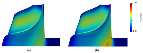
Figure 21.
Normalized von Mises stresses pattern comparison in baseline layout: (a) mechanical versus (b) thermo-mechanical.
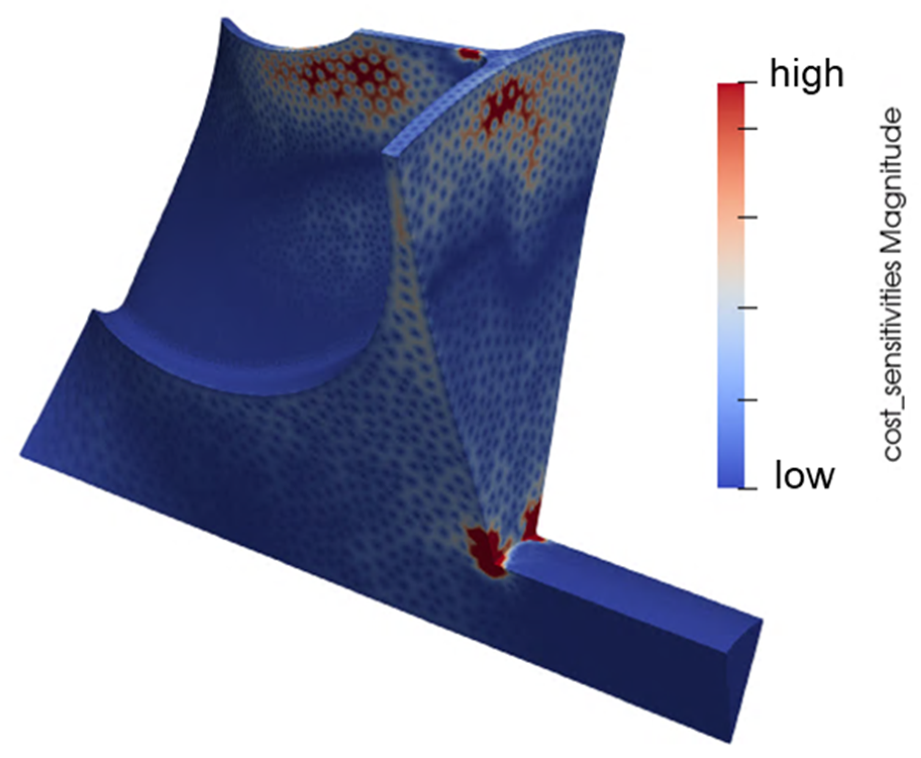
The suitability of the process described in Section 3 is tested with the computation of the sensitivities of the thermo-mechanical constraint w.r.t. the grid coordinates, as reported in Figure 22, providing the information for a grid perturbation. Therefore, Figure 23 compares the distribution of von Mises stresses in the baseline geometry (left) and in the updated layout (right). A local reduction in the maximum von Mises stress in excess of 35% is achieved with the new configuration. Most of the advancements can be attributed to the increased curvature of the back-plate contour, in particular in the region of the connection with the shaft, originally experiencing the highest concentrated stresses. The new shape reveals a more gradual mechanical pattern at such intersection, supported also by a smoother temperature evolution lowering the influence of the local thermal strains. The new layout returns lower sensitivity values, in line with the goal of satisfying the thermo-structural constraint within an optimization problem.

Figure 22.
Sensitivities of the thermo-mechanical constraint w.r.t. grid coordinates.
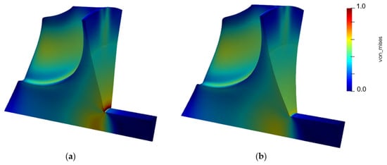
Figure 23.
Normalized von Mises stresses distribution in turbine impeller experiencing thermo-mechanical loading: (a) baseline configuration, (b) updated geometry.
Other areas of the blade are highlighted in Figure 22, in particular at high blade span and in the upper portion of the back-plate. The activation of the sensitivities in such regions is favored by the contribution of the thermal input. However, these portions of the rotor present a pattern of smaller stresses, not violating the original constraint, and therefore their sensitivity fields are neglected.
The second positive effect of the implementation of the CHT analysis within the design loop is about the more accurate prediction of the actual turbine efficiency, as no more adiabatic walls assumptions are in place. The deviation in the total-to-static efficiency w.r.t. an adiabatic simulation is about 0.2% in the selected operative condition while considering the sole impeller. However, more marked differences are expected in case the CHT analysis is extended to the whole turbine stage, including the volute and the nozzle guide vanes.
6. Conclusions
This paper addresses the problem of the Fluid–Structure Interaction in the design optimization of turbomachinery components under thermo-mechanical constraints. The activity focuses on a radial turbine rotor for turbocharger applications, with the aim of reducing the maximum von Mises stress located in a critical area of the impeller experiencing the influence of the thermal loading.
The problem of the integration of high-fidelity thermal predictions within the framework of an optimization is addressed by the development of a novel multidisciplinary gradient-based approach, suitable for the efficient computation of the gradients of the cost function with respect to a large number of design variables. The introduction of a Conjugate Heat Transfer evaluation procedure, supported by the heat transfer forward flux back method, is undertaken in order to establish the energy coupling of the solid domain with its surrounding fluid, according to a partitioned coupling approach. The gradient calculation is addressed by a discrete adjoint technique, and the resulting sensitivities of the thermo-mechanical constraint w.r.t. the grid coordinates allow for the mechanical optimization of the component, including considerations related to the impact of its thermal operative environment.
The solid–fluid grid coupling process, the analysis procedure, and the multidisciplinary differentiation technique are described. Moreover, the validation of the conjugate problem is discussed with reference to the comparison with an analytic solution and a mesh sensitivity study. The accuracy of the computed gradients is also presented.
The application of the multidisciplinary workflow demonstrates the possibility of controlling the local von Mises stresses within admissible ranges, extending the outreach of the original mechanical evaluations with the inclusion of the thermal stresses. New regions of the impeller, before not affected by such considerations, are now involved, as their relative sensitivities are enhanced by the local thermal field. In particular, in the tested sample an improvement exceeding 35% in local von Mises stresses is achieved by the application of the presented method. Additionally, more accurate performance predictions result from the introduction of the CHT analysis within the design optimization process, no more relying on the adiabatic walls assumption.
This contribution is a new step towards the large-scale optimization of turbomachinery components by gradient-based methods, with the goal of the future introduction of fatigue life evaluations in transient conditions.
Author Contributions
Conceptualization, A.R. and T.V.; methodology, A.R. and T.V.; software, A.R.; validation, A.R. and T.V.; formal analysis, A.R.; investigation, A.R.; resources, T.V. and L.C.; writing—original draft preparation, A.R.; writing—review and editing, A.R., T.V., and L.C.; visualization, A.R.; supervision, T.V. and L.C.; project administration, T.V. and L.C.; funding acquisition, T.V. and L.C. All authors have read and agreed to the published version of the manuscript.
Funding
The research leading to these results is co-funded by General Motors Global Propulsion Systems and PUNCH Torino S.p.A. under the grant of the Industrial PhD Program.
Acknowledgments
We gratefully thank General Motors Global Propulsion Systems for the permission to publish this paper.
Conflicts of Interest
The authors declare no conflict of interest. The funders had no role in the collection, analysis, or interpretation of data or in the writing of the manuscript.
Nomenclature
| CFD | Computational Fluid Dynamics |
| FEM | Finite Element Method |
| DWI | Distance-Weighted Interpolation |
| CHT | Conjugate Heat Transfer |
| FSI | Fluid Structure Interaction |
| JT-KIRK | Jacobian Trained Krylov Implicit Runge Kutta |
| MUSCL | Monotonic Upstream-centered Scheme for Conservation Laws |
| design variable | |
| thermal expansion coefficient [K−1] | |
| thermal strain [-] | |
| von Mises stresses [Pa] | |
| adjoint variable | |
| distance between i-th fluid cell-solid node coupling in DWI procedure [m] | |
| temperature gradient normal to wall [K/m] | |
| elasticity-strain matrix | |
| virtual heat transfer coefficient [W/m2 K] | |
| cost function, objective function | |
| thermal conductivity coefficient [W/mK] | |
| heat flux from fluid domain normal to the wall [W/m2] | |
| heat flux in solid domain normal to the wall [W/m2] | |
| non-linear residuals in fluid analysis | |
| fluid temperature in first layer of inner domain cells [K] | |
| virtual fluid bulk temperature [K] | |
| virtual fluid bulk temperature interpolated by DWI procedure [K] | |
| fluid temperature at the wall [K] | |
| fluid temperature in first layer of ghost cells [K] | |
| reference temperature for thermal strains calculation [K] | |
| conservative flow variables in fluid analysis | |
| adjoint variable | |
| primitive flow variables at domain boundaries in fluid analysis | |
| fluid/solid grid coordinate (x,y,z) [m] |
References
- Vassberg, J.C.; Jameson, A. Industrial Application of Aerodynamic Shape Optimization; von Karman Institute for Fluid Dynamics Lecture Series 2018-04; von Karman Institute for Fluid Dynamics: Sint-Genesius-Rode, Belgium, 2018. [Google Scholar]
- Hildebrandt, T.; Thiel, P.; Suganuma, H. Multidisziplinäre und Multikriterielle Kennfeld Optimierung eines Turboladerverdichters für Motorsport Anwendungen. In Proceedings of the 23rd Supercharging Conference, Dresden, Germany, 20–21 September 2018; pp. 355–371. [Google Scholar]
- Fröhlig, F.; Kech, J.; Lachenmaier, N.; Männle, T. The Development of the ZR-Turbocharger-family from MTU to Increase Efficiency and Dynamic of the Charging System. In Proceedings of the 24th Supercharging Conference, Dresden, Germany, 26–27 September 2019; pp. 31–50. [Google Scholar]
- Wöhr, M.; Schneid, M.; Palenschat, T.; Dillmann, A.; Müller, M. Automated Turbocharger Compressor Development at Daimler Trucks. In Proceedings of the 13th International Conference on Turbochargers and Turbocharging, London, UK, 16–17 May 2018; pp. 153–165. [Google Scholar]
- Buske, C.; Krumme, A.; Schmidt, T.; Dresbach, C.; Zur, S.; Tiefers, R. Distributed Multidisciplinary Optimization of a Turbine Blade Regarding Performance, Reliability and Castability. In Proceedings of the ASME Turbo Expo 2016—Volume 2C: Turbomachinery, Seoul, Korea, 13–17 June 2016. [Google Scholar]
- Liu, X.; Furrer, D.; Kosters, J.; Holmes, J. Vision 2040: A Roadmap for Integrated, Multiscale Modeling and Simulation of Materials and Systems; NASA/CR-2018-219771; NASA Technical Reports Server: Washington, DC, USA, 2018.
- Lotz, R.D.; Andrews, D.N.; McHenry, J.P.; Van Saun, D.; Watson, J.P. Further Development of a High-efficiency Compressor Stage Suited to Post Euro VI Emissions and Fuel Economy Legislation. In Proceedings of the 13th International Conference on Turbochargers and Turbocharging, London, UK, 16–17 May 2018; pp. 139–151. [Google Scholar]
- Ioannou, E.; Costall, A.W.; Khairuddin, U.; Ramasamy, P.; Haigh, E. Turbocharger Turbine Aerodynamic Optimization for Reduced Fuel Consumption and CO2 Emissions from Heavy-duty Diesel Engines: Experimental Validation and Flow Field Analysis. In Proceedings of the 13th International Conference on Turbochargers and Turbocharging, London, UK, 16–17 May 2018; pp. 373–388. [Google Scholar]
- Abbas, H.A.; Sarker, R.; Newton, C. PDE: A Pareto-Frontier Differential Evolution Approach for Multi-objective Optimization Problems. In Proceedings of the Congress of Evolutionary Computation, Piscataway, NJ, USA, 27–30 May 2001; Volume 2, pp. 971–978. [Google Scholar]
- Siller, U.; Voβ, C.; Nicke, E. Automated Multidisciplinary Optimization of a Transonic Axial Compressor. In Proceedings of the 47th AIAA Aerospace Sciences Meeting Including The New Horizons Forum and Aerospace Exposition, Orlando, FL, USA, 5–8 January 2009. [Google Scholar]
- Goldberg, D.E. Genetic Algorithms in Search, Optimization and Machine Learning; Addison-Wesley Longman Publishing: Boston, MA, USA, 1989. [Google Scholar]
- Conn, A.R.; Scheinberg, K.; Vicente, L.N. Introduction to Derivative-Free Optimization; MOS-SIAM Series on Optimization; SIAM: Philadelphia, PA, USA, 2009. [Google Scholar]
- Trunk, G.V. A Problem of Dimensionality: A Simple Example. IEEE Transaction on Pattern Analysis and Machine Intelligence; IEEE: Piscataway, NJ, USA, 1979; Volume 1, Issue 3, pp. 306–307. [Google Scholar]
- Jameson, A. Aerodynamic Design via Control Theory. J. Sci. Comput. 1988, 3, 233–260. [Google Scholar] [CrossRef]
- Giles, M.B.; Pierce, N.A. An Introduction to the Adjoint Approach to Design. Flow Turbul. Combust. 2000, 65, 393–415. [Google Scholar] [CrossRef]
- Martins, J.R.R.A.; Sturdza, P.; Alonso, J.J. The Complex-step Derivative Approximation. In ACM Transactions on Mathematical Software; Association for Computing Machinery: New York, NY, USA, 2003; Volume 29, Issue 3. [Google Scholar]
- Luo, J.; Xiong, J.; Liu, F.; McBean, I. Three-Dimensional Aerodynamic Design Optimization of a Turbine Blade by Using an Adjoint Method. J. Turbomach. 2011, 133, 011026. [Google Scholar] [CrossRef]
- Pironneau, O. On Optimum Design in Fluid Mechanics. J. Fluid Mech. 1974, 64, 97–110. [Google Scholar] [CrossRef]
- Mueller, L. Adjoint-Based Optimization of Turbomachinery Applied to Axial and Radial Turbines. Ph.D. Thesis, Université Libre de Bruxelles, Bruxelles, Belgium, 2019. [Google Scholar]
- Verstraete, T.; Mueller, L.; Mueller, J.D. CAD-Based Adjoint Optimization of the Stresses in a Radial Turbine. In Proceedings of the ASME Turbo Expo 2017, Charlotte, NC, USA, 26–30 June 2017; Volume 2C. Paper No. GT2017-65005. [Google Scholar]
- Schwalbach, M.; Mueller, L.; Verstraete, T.; Gauger, N.R. CAD-Based Adjoint Multidisciplinary Optimization of a Radial Turbine under Structural Constraints. In Proceedings of the 2018 Global Power and Propulsion Forum, Montreal, QC, Canada, 10–12 January 2018. Paper No. GPPS-NA-2018-133. [Google Scholar]
- Mueller, L.; Prinsier, J.; Verstraete, T.; Racca, A. CAD-Based Multidisciplinary Adjoint Optimization of a Radial Compressor Impeller. In Proceedings of the 24th Supercharging Conference, Dresden, Germany, 26–27 September 2019; pp. 415–434. [Google Scholar]
- Pini, M.; Persico, G.; Dossena, V. Robust Adjoint-Based Shape Optimization of Supersonic Turbomachinery Cascades. In Proceedings of the ASME Turbo Expo, Dusseldorf, Germany, 16–20 June 2014. [Google Scholar]
- Lachenmaier, N.; Baumgärtner, D.; Schiffer, H.P.; Kech, J. Gradient-free and Gradient-based Optimization of a Radial Turbine. In Proceedings of the 13th European Conference on Turbomachinery Fluid dynamics & Thermodynamics, Lausanne, Switzerland, 8–12 April 2019. [Google Scholar]
- He, L.; Wang, D.X. Concurrent Blade Aerodynamic-Aero-elastic Design Optimization Using Adjoint Method. J. Turbomach. 2011, 133, 011021. [Google Scholar] [CrossRef]
- Xu, S.; Radford, D.; Meyer, M.; Mueller, J.D. Stabilisation of Discrete Steady Adjoint Solvers. J. Comput. Phys. 2015, 299, 175–195. [Google Scholar] [CrossRef]
- Xu, S.; Timme, S. Robust and Efficient Adjoint Solver for Complex Flow Conditions. Comput. Fluids 2017, 148, 26–38. [Google Scholar] [CrossRef]
- Rakut, C.; Diefenthal, M.; Tadesse, H.; Wirsum, M. Radial Turbine Temperature Field; FVV Information Sessions Turbomachinery, Project 1064; FVV: Würzburg, Germany, 2015. [Google Scholar]
- Makhija, D.S.; Beran, P.S. Concurrent Shape and Topology Optimization for Unsteady Conjugate Heat Transfer. Struct. Multidiscip. Optim. 2020, 62, 1275–1297. [Google Scholar] [CrossRef]
- Jaksch, P. Implementation of an Adjoint Thermal Solver for Inverse Problems. In Proceedings of the 12th European Conference on Turbomachinery Fluid Dynamics & Thermodynamics, Stockholm, Sweden, 3–7 April 2017. [Google Scholar]
- Subramaniam, V.; Dbouk, T.; Harion, J.-L. Topology Optimization of Conjugate Heat Transfer Systems: A Competition between Heat Transfer Enhancement and Pressure Drop Reduction. Int. J. Heat Fluid Flow 2019, 75, 165–184. [Google Scholar] [CrossRef]
- Perelmann, L.T. On Conjugate Problems of Heat Transfer. Int. J. Heat Mass Transf. 1961, 3, 293–303. [Google Scholar] [CrossRef]
- Luikov, A.V. Conjugate Convective Heat Transfer Problems. Int. J. Heat Mass Transf. 1974, 17, 257–265. [Google Scholar] [CrossRef]
- Verstraete, T. CADO: A Computer Aided Design and Optimization Tool for Turbomachinery Applications. In Proceedings of the 2nd International Conference on Engineering Optimization, Lisbon, Portugal, 6–9 September 2010; pp. 6–9. [Google Scholar]
- Nocedal, J.; Wright, S.J. Numerical Optimization; Springer Science & Business Media, LLC: Berlin/Heidelberg, Germany, 2006; Volume 2. [Google Scholar]
- Gkaragkounis, K.T.; Papoutsis-Kiachagias, E.M.; Giannakoglou, K.C. The Continuous Adjoint Method for Shape Optimization in Conjugate Heat Transfer Problems with Turbulent Incompressible Flows. Appl. Therm. Eng. 2018, 140, 351–362. [Google Scholar] [CrossRef]
- Mousavi, S.A. Constrained Aerodynamic and Heat Transfer Optimization of Gas Turbine Blades Using an Adjoint Approach. Ph.D. Thesis, McGill University, Montreal, QC, Canada, 2012. [Google Scholar]
- Burghardt, O.; Albring, T.; Gauger, N.R. Computation of Accurate Adjoint-based Gradients for Optimization in Conjugate Heat Transfer Problems. In Proceedings of the 6th European Conference on Computational Mechanics, Glasgow, UK, 11–15 June 2018. [Google Scholar]
- Burghardt, O.; Gauger, N.R.; Economon, T.D. Coupled Adjoints for Conjugate Heat Transfer in Variable Density Incompressible Flows. In Proceedings of the AIAA Aviation 2019 Forum, Dallas, TX, USA, 17–21 June 2019. [Google Scholar]
- Towara, M.; Lotz, J.; Naumann, U. Discrete Adjoint Approaches for CHT Applications in OpenFOAM. In Proceedings of the Eurogen 2019, Guimarães, Portugal, 12–14 September 2019. [Google Scholar]
- Verdicchio, J.A.; Chew, J.W.; Hills, N.J. Coupled Fluid/Solid Heat Transfer Computation for Turbine Discs. In Proceedings of the ASME Turbo Expo, New Orleans, LA, USA, 4–7 June 2001; Volume 3. Paper No. 2001-GT-0205. [Google Scholar]
- Errera, M.P.; Baqué, B. A Quasi-dynamic Procedure for Coupled Thermal Simulations. Int. J. Numer. Methods Fluids 2013, 72, 1183–1206. [Google Scholar] [CrossRef]
- Sun, Z.; Chew, J.W.; Hills, N.J.; Volkov, K.N.; Barnes, C.J. Efficient Finite Element Analysis/Computational Fluid Dynamics Thermal Coupling for Engineering Applications. J. Turbomach. 2010, 132, 031016. [Google Scholar] [CrossRef]
- Meng, F.; Dong, S.; Wang, J.; Guo, D. A New Algorithm of Global Tightly-coupled Transient Heat Transfer Based on Quasi-steady Flow to the Conjugate Heat Transfer Problem. Theor. Appl. Mech. Lett. 2016, 6, 233–235. [Google Scholar] [CrossRef]
- Radenac, E.; Gressier, J.; Millan, P.; Giovannini, A. A Conservative Coupling Numerical Method for Transient Conjugate Heat Transfer. In Proceedings of the International Conference on Computational Methods for Coupled Problems in Science and Engineering, Santorin, Greece, 25–28 May 2005. [Google Scholar]
- Verstraete, T. Multidisciplinary Turbomachinery Component Optimization Considering Performance, Stress, and Internal Heat Transfer. Ph.D. Thesis, Universiteit Gent, Gent, Belgium, 2008. [Google Scholar]
- Verstraete, T.; Van den Braembussche, R. A Novel Method for the Computation of Conjugate Heat Transfer with Coupled Solvers. In Proceedings of the International Symposium on Heat Transfer in Gas Turbine Systems, Antalya, Turkey, 9–14 August 2009. [Google Scholar]
- Verstraete, T.; Scholl, S. Stability Analysis of Partitioned Methods for Predicting Conjugate Heat Transfer. Int. J. Heat Mass Transf. 2016, 101, 852–869. [Google Scholar] [CrossRef]
- Bathe, K.J.; Khoshgoftaar, M.R. Finite Element Formulation and Solution of Nonlinear Heat Transfer. Nucl. Eng. Des. 1979, 51, 389–401. [Google Scholar] [CrossRef]
- Blazek, J. Computational Fluid Dynamics: Principles and Applications, 2nd ed.; Elsevier Science Ltd.: Amsterdam, The Netherlands, 2001. [Google Scholar]
- Schwalbach, M.; Verstraete, T.; Gauger, N.R. Adjoint Optimization of Turbomachinery Components under Mechanical Constraints. In The 8th VKI PhD Symposium; von Karman Institute for Fluid Dynamics: Sint-Genesius-Rode, Belgium, 2007. [Google Scholar]
- Dhondt, G. The Finite Element Method for Three-Dimensional Thermomechanical Applications; John Wiley & Sons Ltd.: Chichester, UK, 2004. [Google Scholar]
- Martins, J.R.R.A.; Alonso, J.J.; Reuther, J.J. A Coupled-Adjoint Sensitivity Analysis Method for High-Fidelity Aero-Structural Design. Optim. Eng. 2005, 6, 33–62. [Google Scholar] [CrossRef]
- Griewank, A.; Walther, A. Evaluating Derivatives: Principles and Techniques of Algorithmic Differentiation, 2nd ed.; Siam: Philadelphia, PA, USA, 2008. [Google Scholar]
- Scholl, S.; Janssens, B.; Verstraete, T. Stability of Static Conjugate Heat Transfer Coupling Approaches Using Robin Interface Conditions. Comput. Fluids 2018, 172, 209–225. [Google Scholar] [CrossRef]
- Hirsch, C. Numerical Computation of Internal and External Flows, Volume 2: Computational Methods for Inviscid and Viscous Flows; Wiley: Chichester, UK, 1990. [Google Scholar]
- Taguchi, G. Introduction to Quality Engineering: Designing Quality into Products and Processes; Asian Productivity Organization/UNIPUB: White Plain, NY, USA; Unipub/Kraus: New York, NY, USA, 1986. [Google Scholar]
Publisher’s Note: MDPI stays neutral with regard to jurisdictional claims in published maps and institutional affiliations. |
© 2020 by the authors. Licensee MDPI, Basel, Switzerland. This article is an open access article distributed under the terms and conditions of the Creative Commons Attribution (CC BY) license (http://creativecommons.org/licenses/by/4.0/).

