4.2. Rotor Mesh Sensitivity Analysis
A mesh sensitivity study for the CHT analysis is performed on a three-dimensional test case presented in [
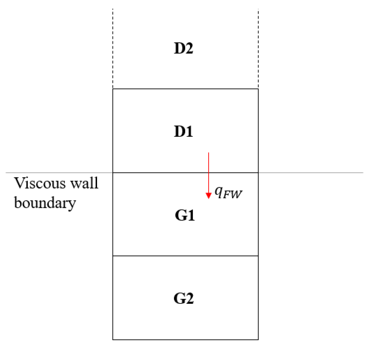
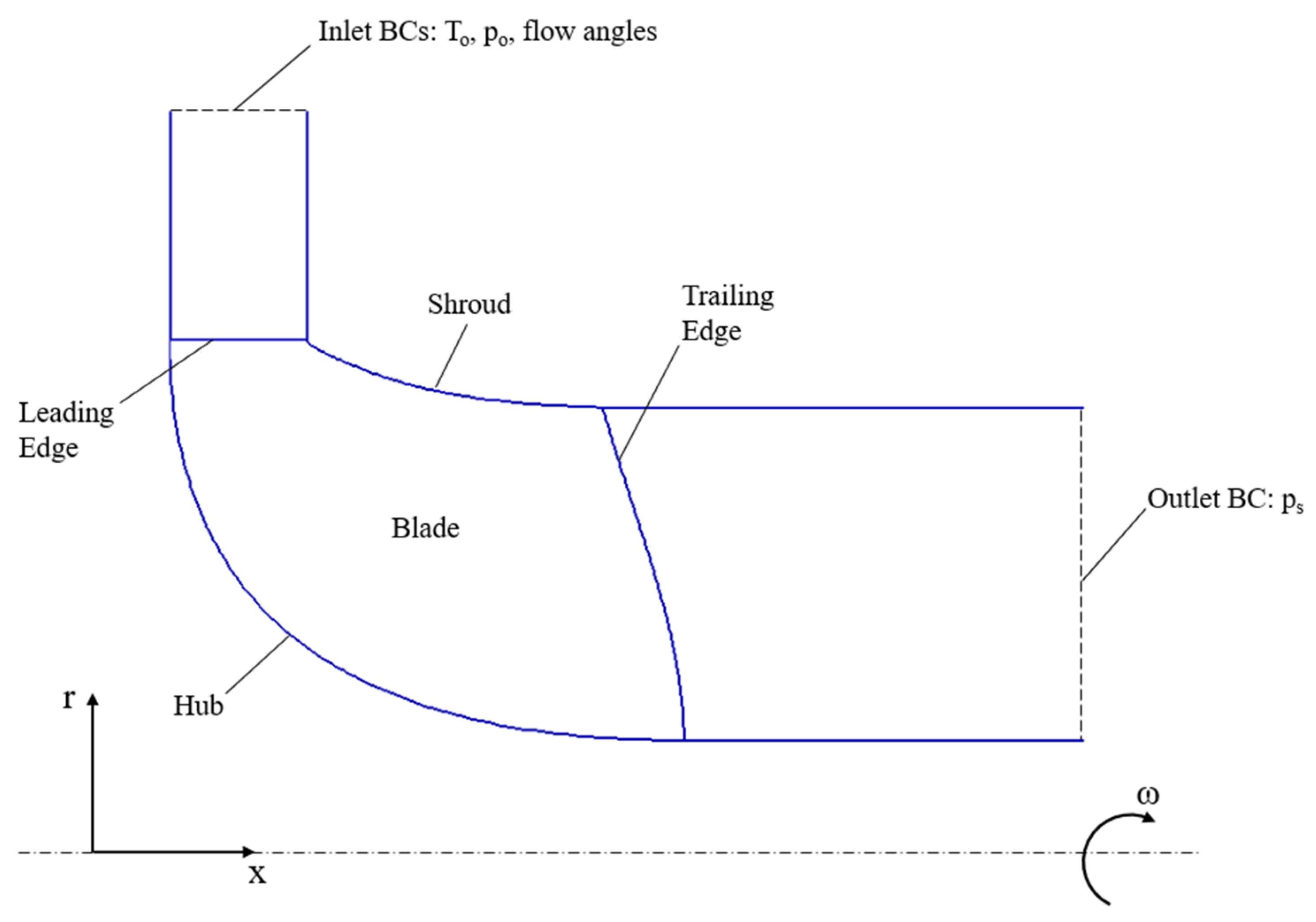
19], considering a radial turbine impeller with 10 blades and an inlet diameter of 50 mm. A two-dimensional sketch of the domain on the meridional plane of the rotor is reported in
Figure 11, along with the locations of the imposed boundary conditions. The method of the characteristics [
56] is adopted to establish the number of physical conditions to be assigned at the inflow and outflow boundaries. The total upstream temperature and pressure are specified at the inlet of the domain, along with flow velocity components in the corresponding coordinate system. At the subsonic outflow boundary, a single flow variable is imposed, specifically the downstream static pressure. In conclusion, the boundary conditions applied to the problem are summarized in
Table 2, in which the impeller rotational speed is also included.
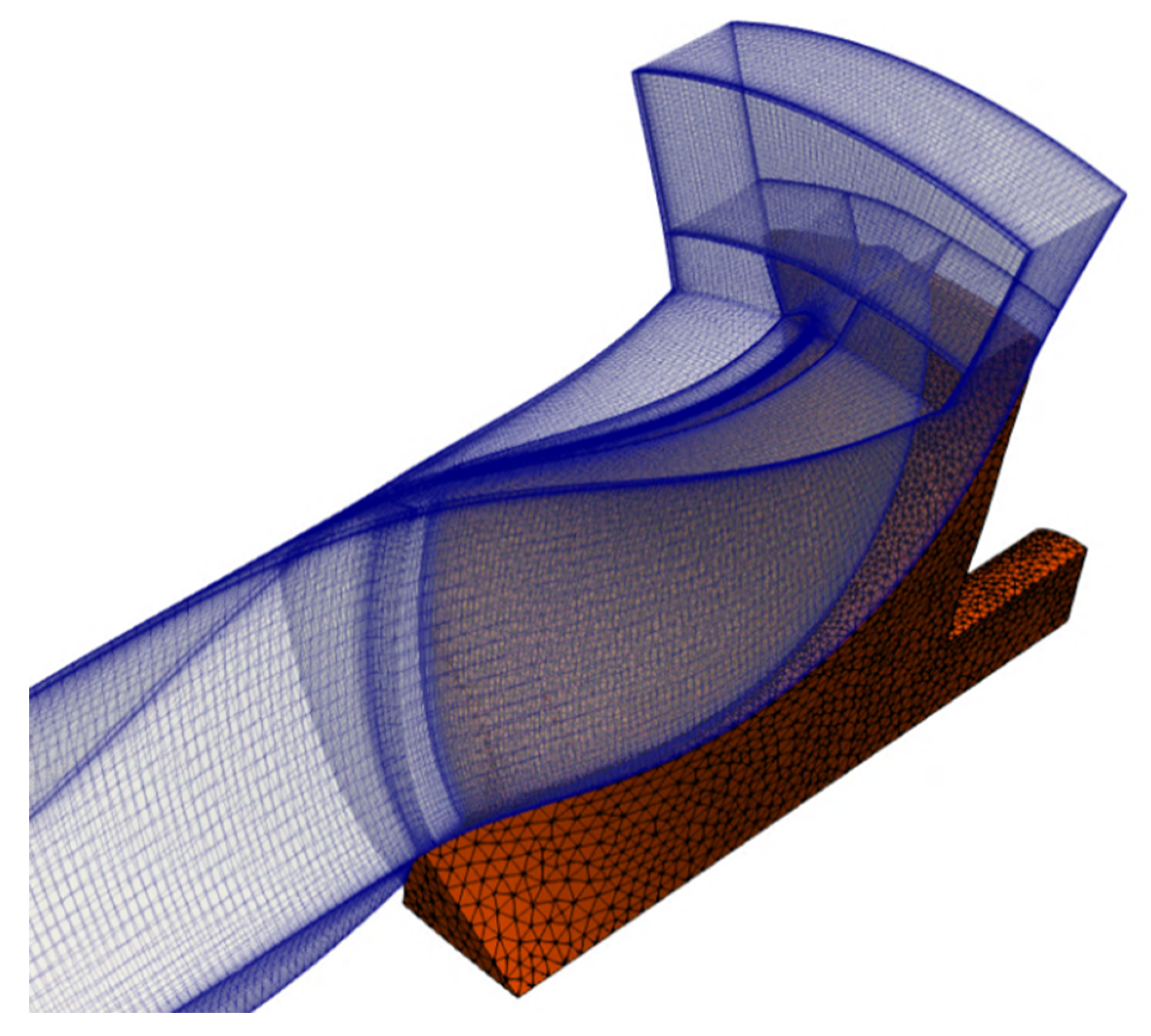
The interactions of the rotor fluid and solid meshes are explored over three levels of refinement, as summarized in
Table 3. Additionally, three values of the virtual heat transfer coefficient
are investigated in order to determine a suitable trade-off between stability and computational time. These factors are explored following the combinations expressed by the L9 Orthogonal Array method [
57], returning nine test cases (
Table 4).
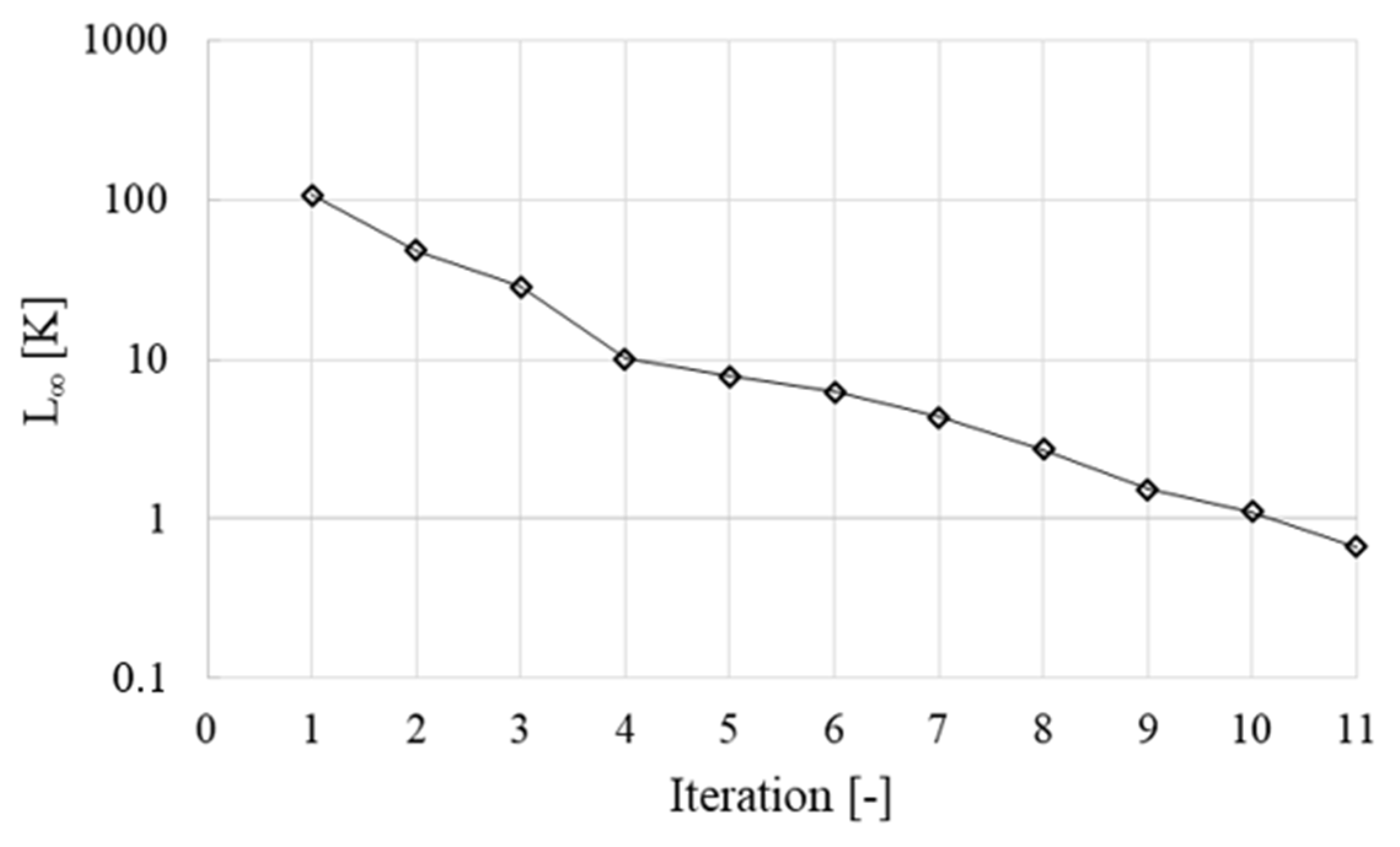
All the simulations are run till convergence at a relative residual drop of 10−8 for the computational fluid dynamics (CFD) solver and 10−10 for the FEM solver, while the CHT workflow is stopped for a maximum deviation in wall temperature between two successive fluid-solid iterations L∞ below 1 K. y+ values below unity are obtained for the “mid” and “fine” levels of the fluid grid refinement, while the coarsest one exhibits a peak in y+ around 2.5 at the blade leading edge. Concerning the maximum number of nodes in the solid mesh, the code was tested up to the finest possible grid before incurring in memory leakage issues with the adopted Conjugate Gradient iterative solver.
The results in
Table 5 demonstrate a low sensitivity of the maximum temperature in the solid domain due to the settings applied to the coupling process, except for the first test case with coarse meshes at both the fluid and solid side. A critical aspect is represented by the quality of the interpolation of the information between the two domains realized by the fine-tuned distribution of virtual grid points on the interface at fluid side, as discussed in
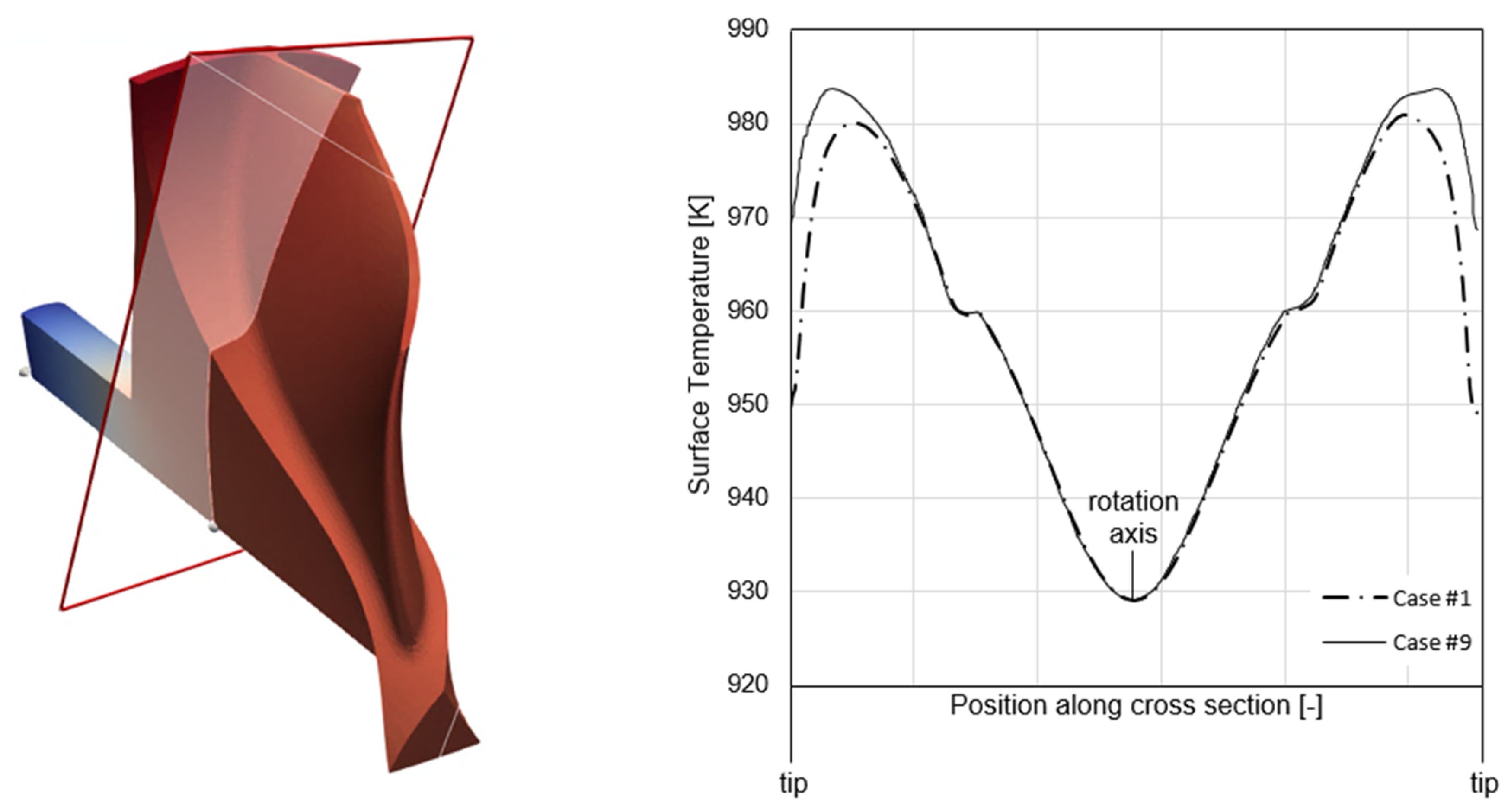
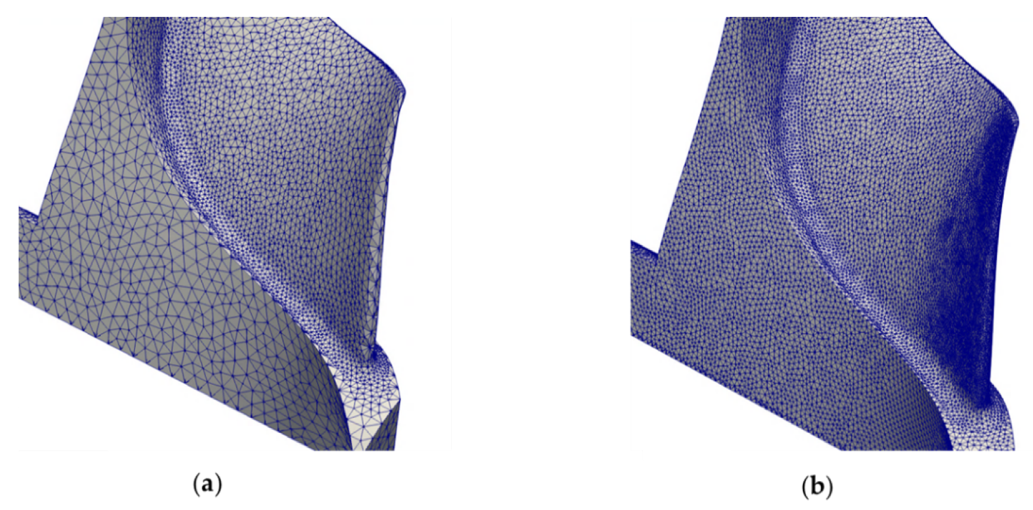
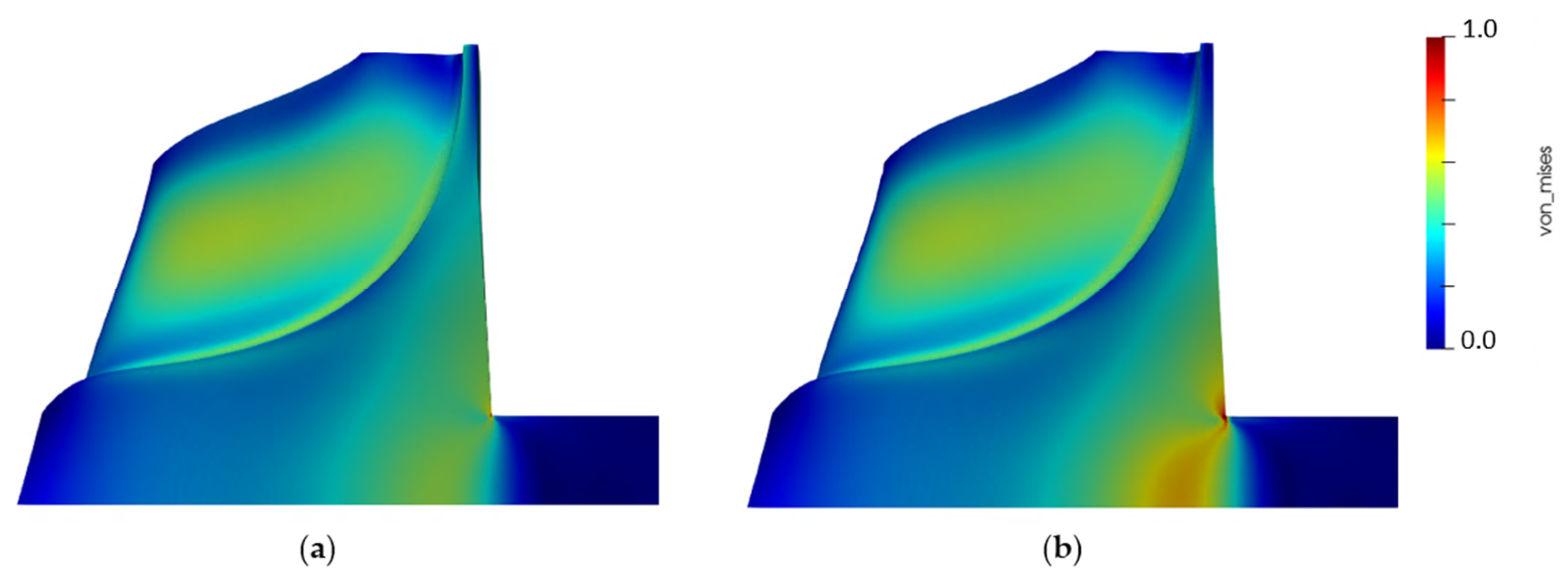
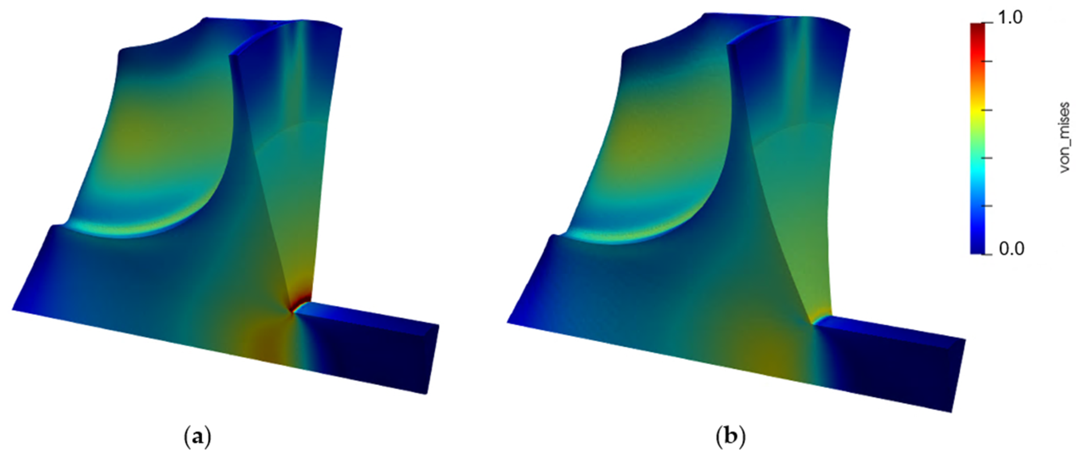
Section 2.1. Moreover, the finest solid mesh increases the resolution of the convective loading, resulting in more accurate temperature predictions in the material and, therefore, also more reliable heat fluxes returned to the fluid. Figure 14 shows two cases of solid mesh size, the coarse one (Figure 14a) and the intermediate one (Figure 14b), with the addition of the trailing edge refinement described hereafter. In the case of finer solid grids, the interpolation procedure returns a richer temperature pattern at the interface, closely mirroring the fluid conditions at the walls, whilst the coarsest one approximates the thermal loading distribution with the highest deviations localized in the blade tip region, where large secondary flows and leakages are present, and at the trailing edge. In this respect, a surface temperature analysis at a cross section located at about 25% of the chord was performed in order to evaluate the integral of the temperature deviations between each investigated test case w.r.t. test case 9. The axial position of the planar section was chosen in a region of high convective perturbations due to the presence of a significant flow detachment at the blade leading edge. The results, summarized in
Table 5, are supported by the example in
Figure 12, showing the temperature contours for case 1 and case 9. It is interesting to note that, in both set-ups, the blade tip returns significant thermal gradients because of the thinner geometry exposed to the flow vortices. However, the coarsest mesh overestimates the temperature drop, resulting in the integral reported in
Table 5.
Finally, considerations about the computational time are synthesized in
Table 5, with a dominant portion covered by the CFD solver and a significant rise in overhead emerging from the FEM heat transfer computations at the finest grid level. The normalization refers to the total duration of a single CHT iteration, including also the hFFB procedure. The comparison is performed w.r.t. the reference duration of test case 1, presenting the coarsest meshes at both fluid and solid side.
The interactions among the three factors in the Orthogonal Array from
Table 4 are studied through the compounded signal
S, defined as:
with the term
A enclosing the normalized difference between the maximum temperature predicted by the test case of interest and test case 9 (showing the finest grids),
B representing the normalized computational time, and ω as the weighting coefficient. In the current study, ω = 0.7 in order to bias the objective function towards the accuracy of the coupling process. Indeed, the factors levels finally expected from this study are the ones minimizing the signal
S.
The analysis of the Orthogonal Array [
57], resulting in
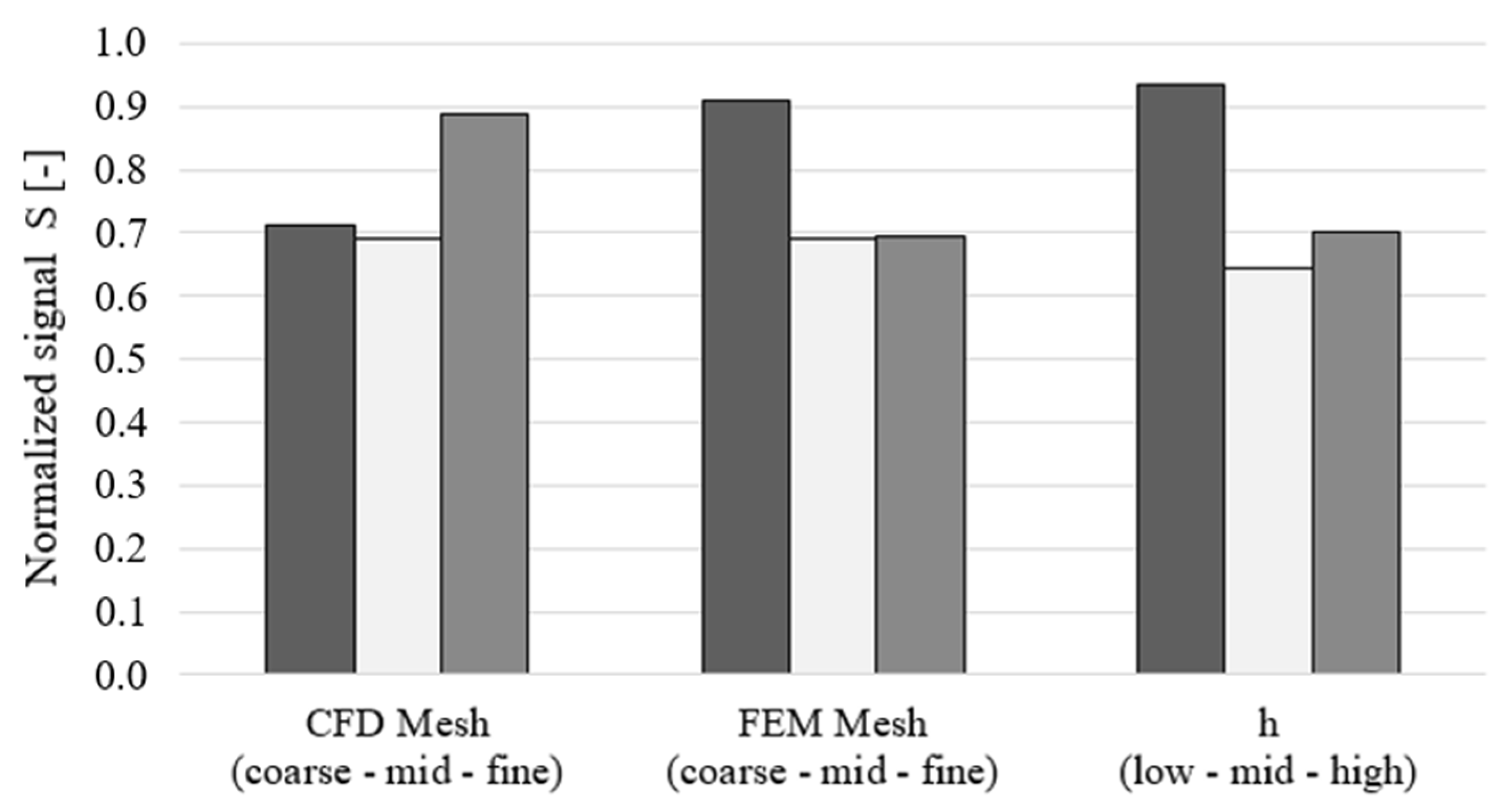
Figure 13, reveals the dependence of the signal
S from the three variables and their correspondent levels. The chart illustrates the virtual heat transfer coefficient
is selected at its highest value within the stability region of the Biot number discussed in [
46], as it influences the
B term in Equation (36), determining the rate of convergence of the CHT coupling process. Indeed, the current problem exhibits an optimal
= 1000 W/m
2 K, since the highest value approaches the limit of the stability region, with incipient oscillations in the value of heat flux exchanged at the interface, before reaching convergence. The solid grid size, instead, characterizes the accuracy of the interpolation of the quantities passed between the two domains through the DWI process and affects the
A term in Equation (36). In general, finer solid grids are favored by the current analysis. Remarkably, the fluid mesh size follows an opposite trend because its influence on the
A term is less pronounced, as the coarsest level already provides good-quality solutions. On the other hand, the signal
S is driven by the increase in computational overhead experienced with the fluid mesh refinement.
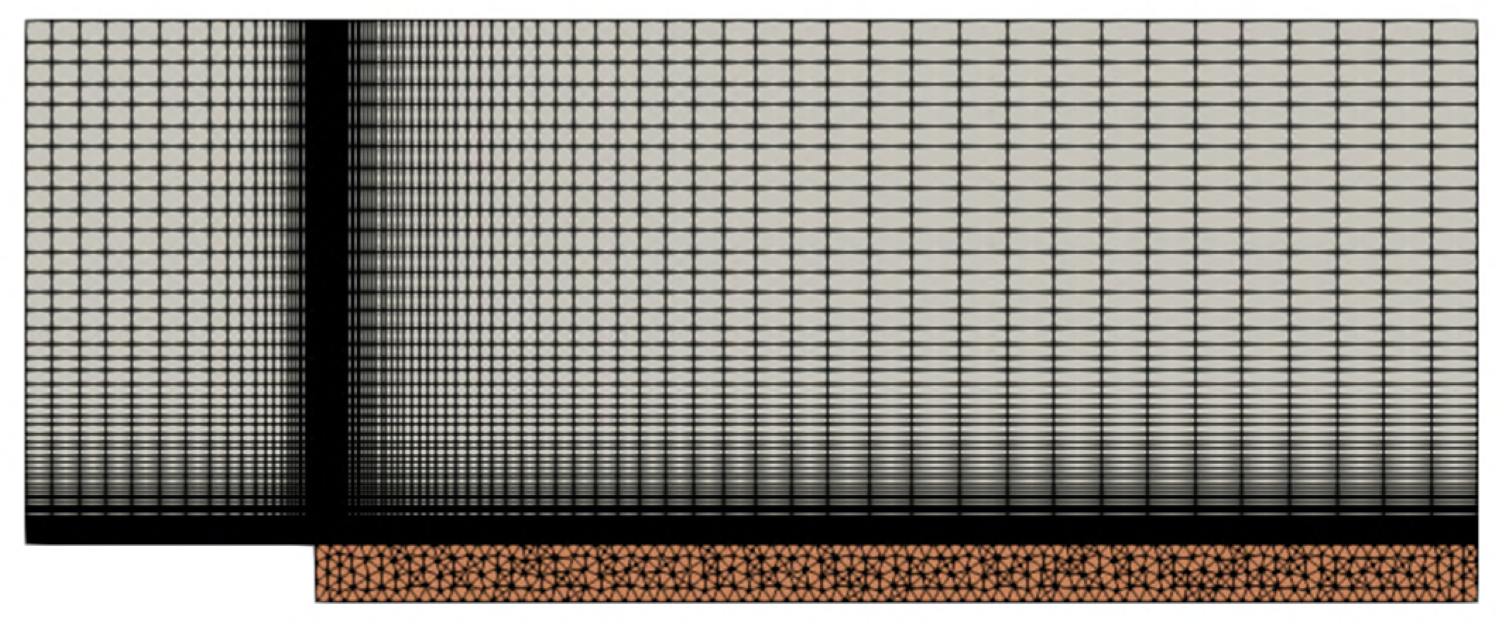
Since the weighting coefficient ω privileges the accuracy of the CHT coupling process, the final selection of the factors levels results in the intermediate values for the refinements of both the grids and for the virtual heat transfer coefficient. However, it is recognized that smaller solid element sizes improve the stability of the CHT coupling process because it avoids local poor quality in the discretization of the blade surface in correspondence with thin regions (
Figure 14a), potentially inducing drops in the local Biot number and inconsistencies with the selected
value from a stability standpoint. Therefore, the issue is addressed by the generation of a “hybrid” configuration (
Figure 14b), envisaging a local solid mesh refinement in correspondence with the blade tip surface and trailing edge, whilst maintaining the intermediate element size in the rest of the domain. This last setup increases the mesh density to a total node count of about 420 k.
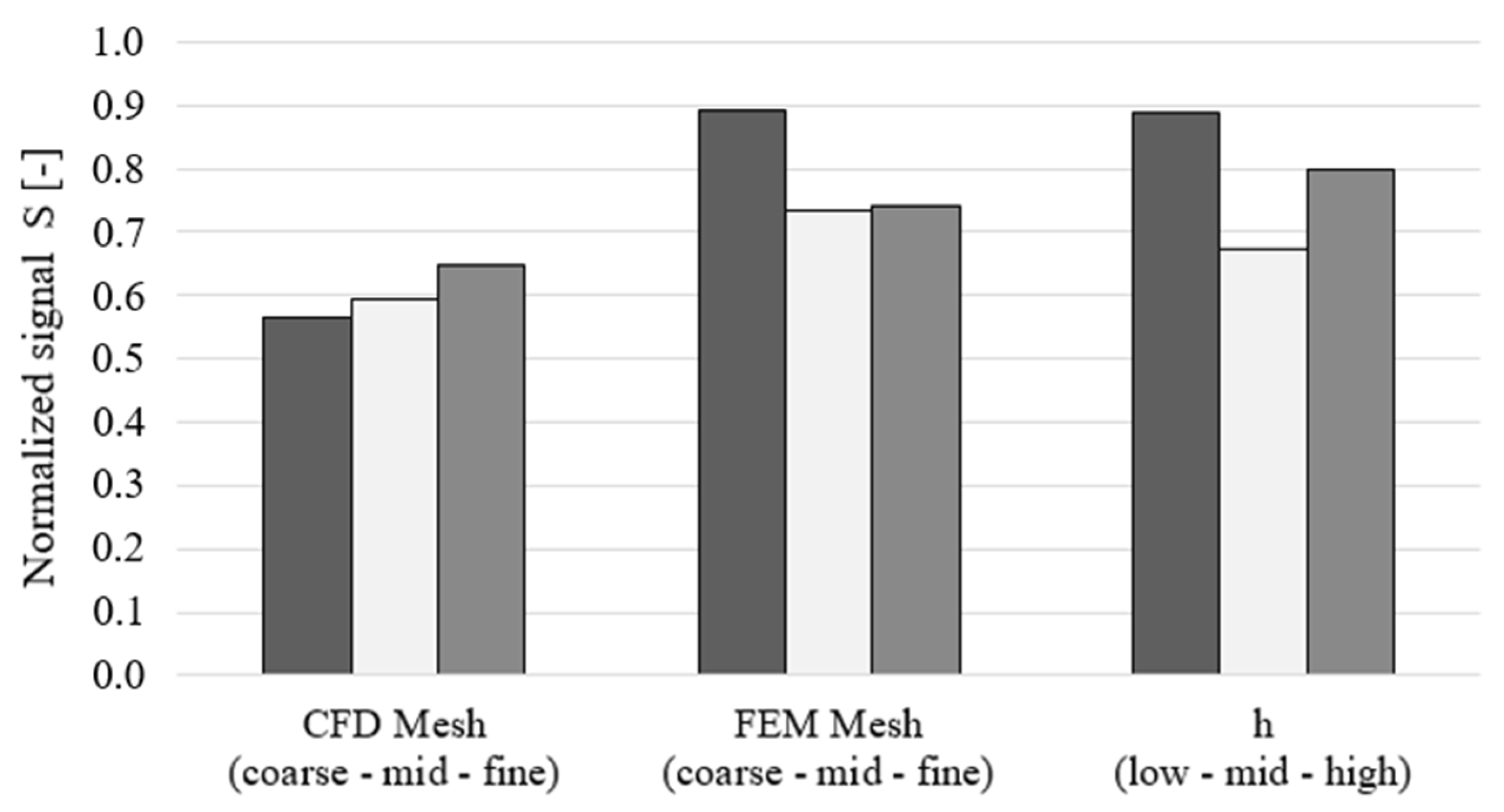
Finally, the Orthogonal Array analysis is repeated, assigning the integral of temperature deviations to the
A term in Equation (36). The outcome, shown in
Figure 15, confirms the previous considerations, except for the fluid mesh size, which promotes the trend towards the coarsest mesh because it still provides sufficiently accurate results. However, since the difference between the coarse and intermediate meshes is moderate, the previous selection of the medium size grid will be pursued for the sake of improved prediction accuracy.
Based on such considerations, the settings returned by the analysis of the Orthogonal Array are considered for the further assessments of the coupling problem.
4.3. Gradients Accuracy Evaluation
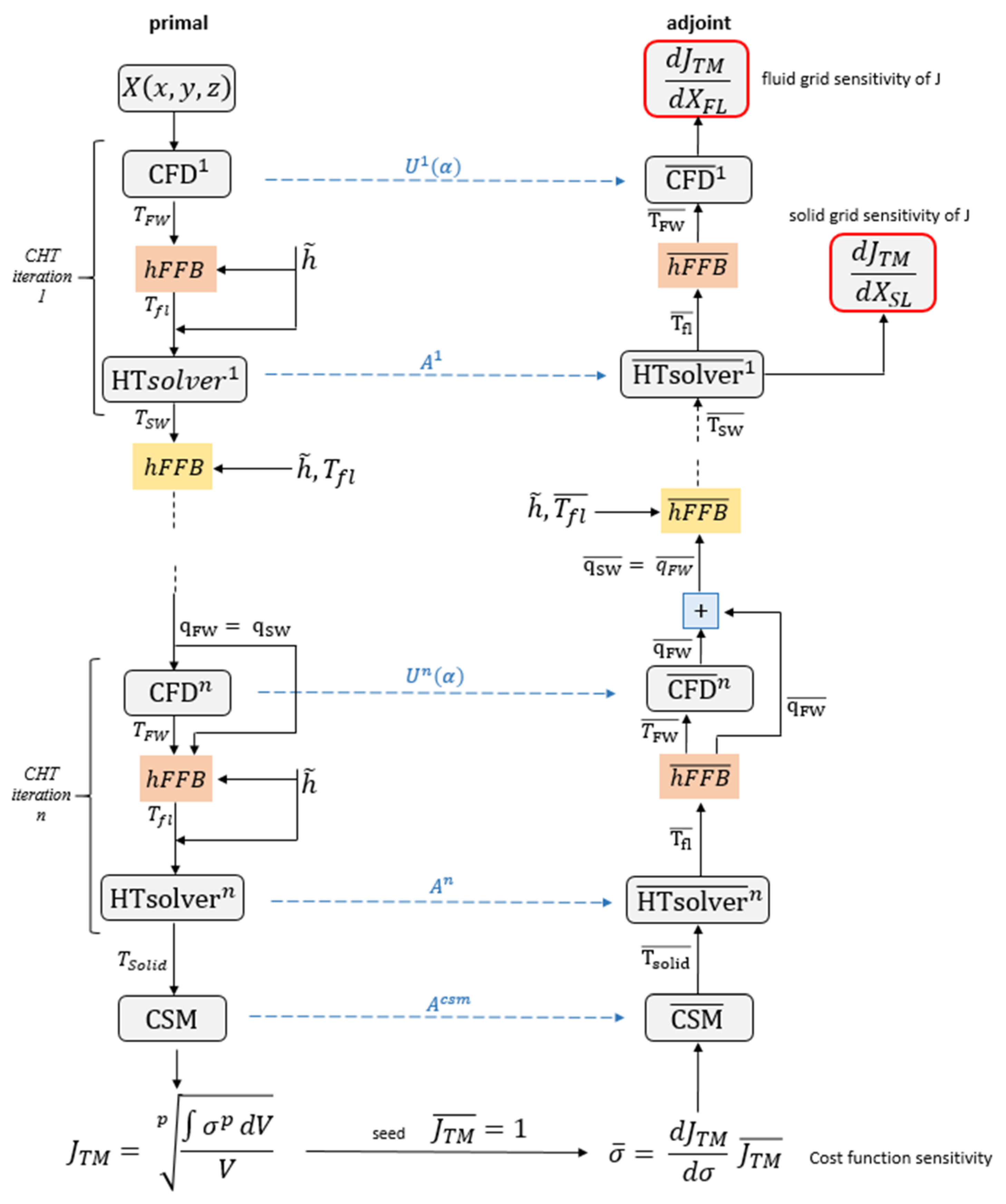
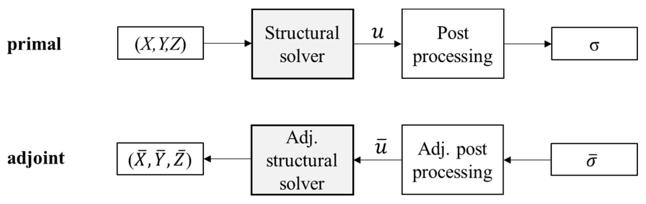
The present work accounts for the manual differentiation of the multidisciplinary process shown in
Figure 6. The sensitivities are accurately computed by the reverse Algorithmic Differentiation technique [
54] for what concerns the FEM solvers and the hFFB process, while the partitioned coupling approach opens the path to the direct integration of the in-house adjoint CFD solver.
The validation of the differentiated FEM solvers is presented herein with reference to the rotor test case from
Section 4.2. The adjoint sensitivities
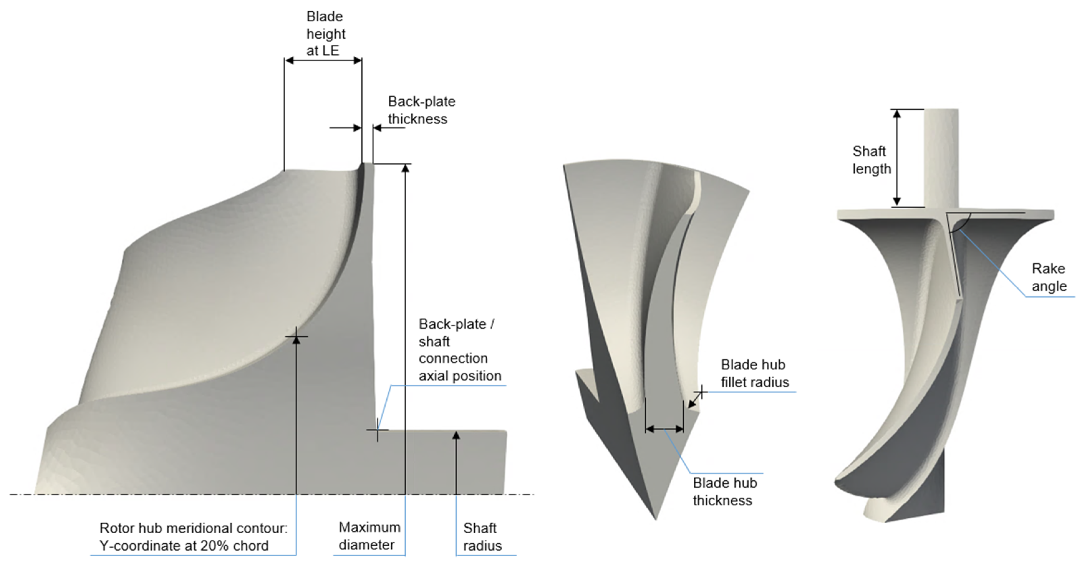
of the maximum temperature and of the maximum von Mises stress including the thermal strain w.r.t. selected design parameters (referenced in
Table 6 and
Figure 16) are compared to the correspondent gradients computed by the Finite Differences (FD) technique. The latter accounts for evaluations by a central differencing scheme, whose optimal step size is searched with the aim of accurate gradients computations. An exemplary case is reported in
Figure 17, showing the identification of a suitable step size at the value of 10
−6 m for the seventh design variable in the framework of thermal evaluations by the heat transfer solver. The magnitude of the perturbation must avoid too-small values, resulting in round-off errors, and too large values as well, because they introduce significant truncation errors. This outcome results from the evaluation of the cost function at each step size by solving the linear system obtained after the perturbation of the mesh through the morphing technique described in [
20].
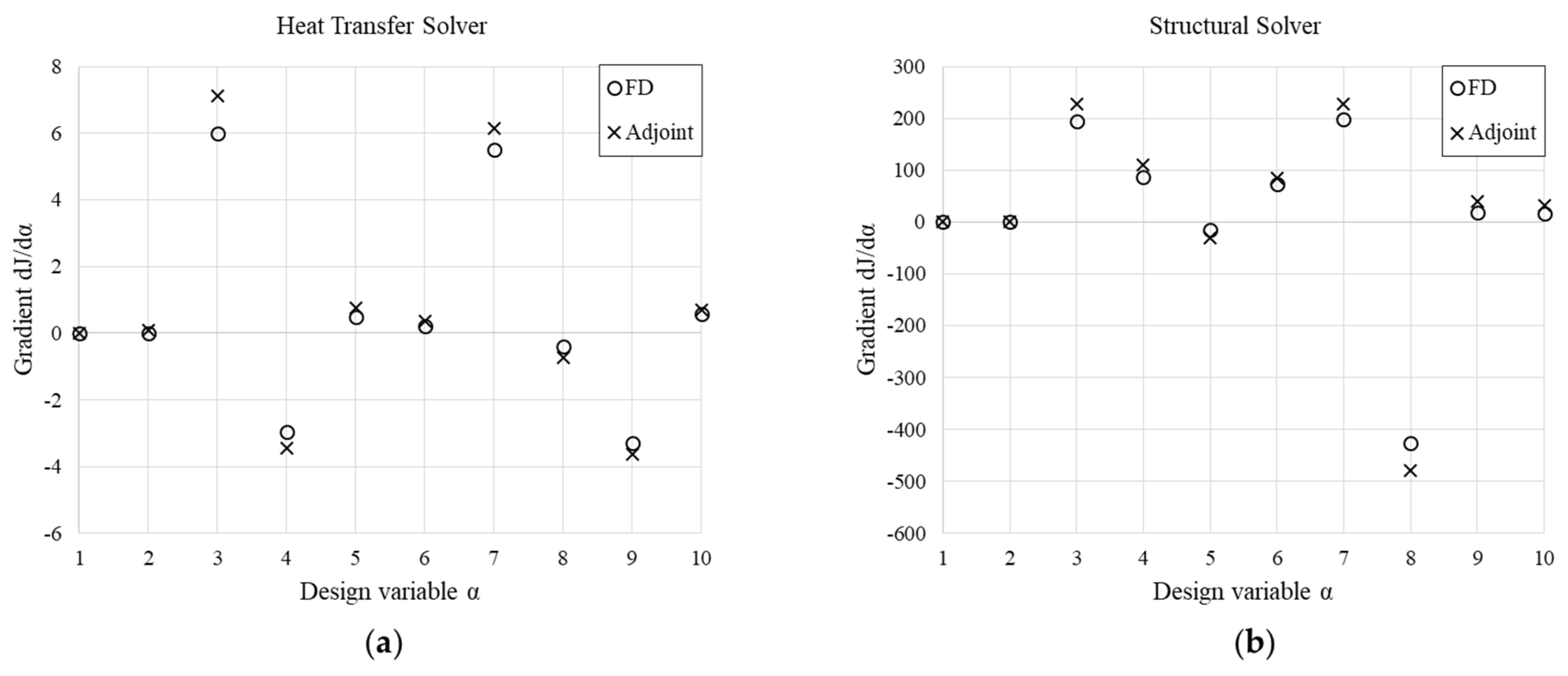
The sensitivities of the maximum solid temperature to perturbations of the ten design variables are summarized in
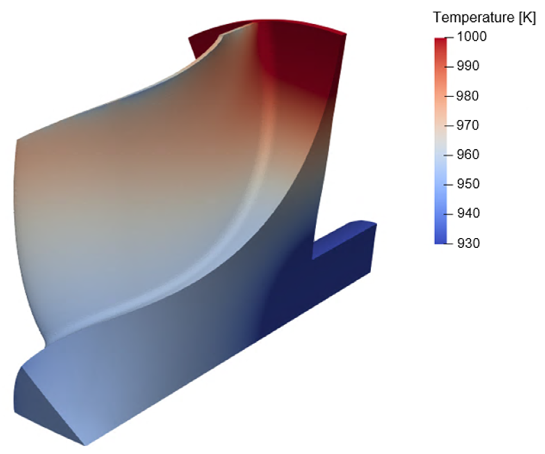
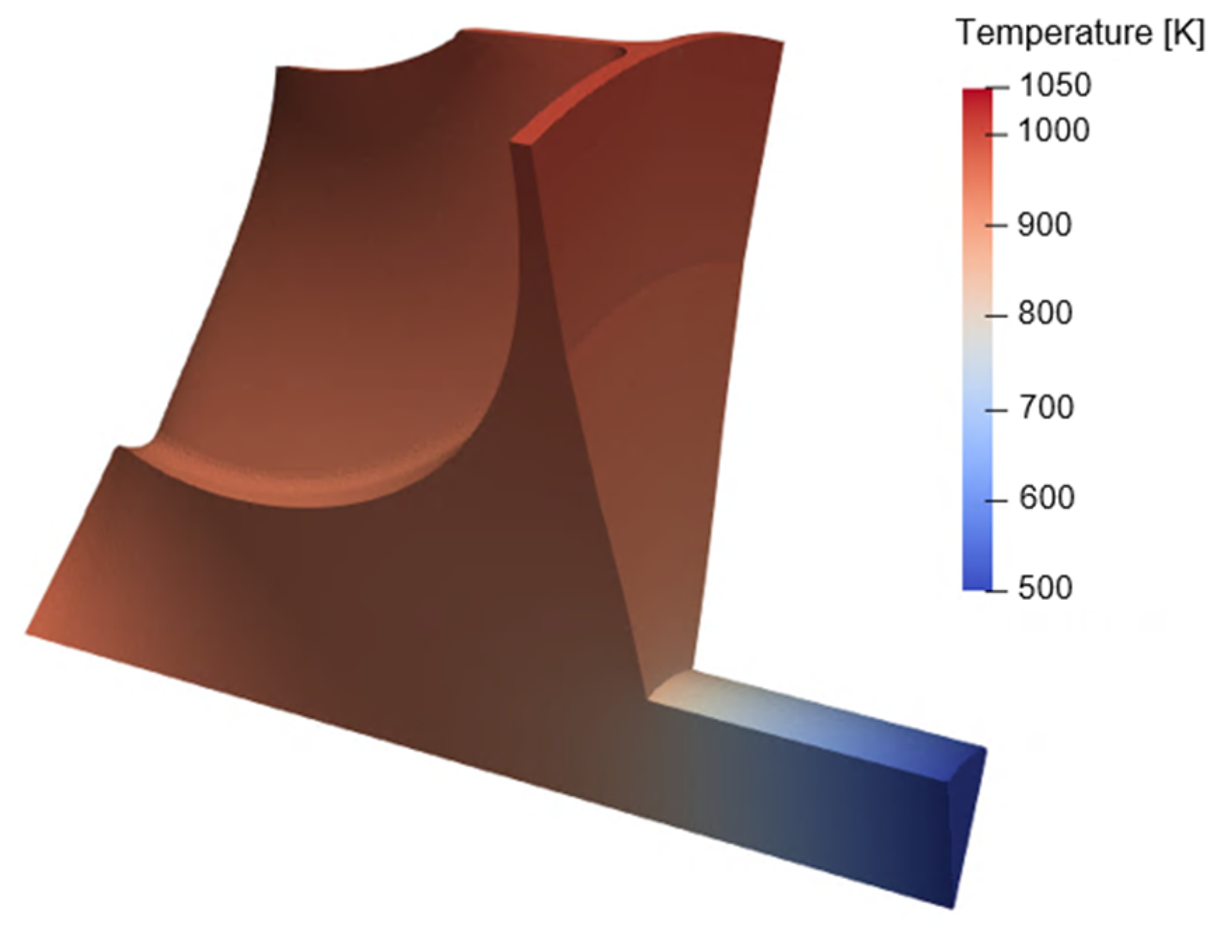
Figure 18a, which shows a close agreement between the two methods, both in sign and magnitude. To understand the sensitivity analysis in detail, let us consider the thermal paths in the turbine rotor experiencing the convective loading resulting from the operative condition reported in
Table 2, along with a convective condition on the back-plate surface with a uniform fluid temperature of 950 K and a Dirichlet boundary condition of 500 K assigned to the extreme section of the shaft.
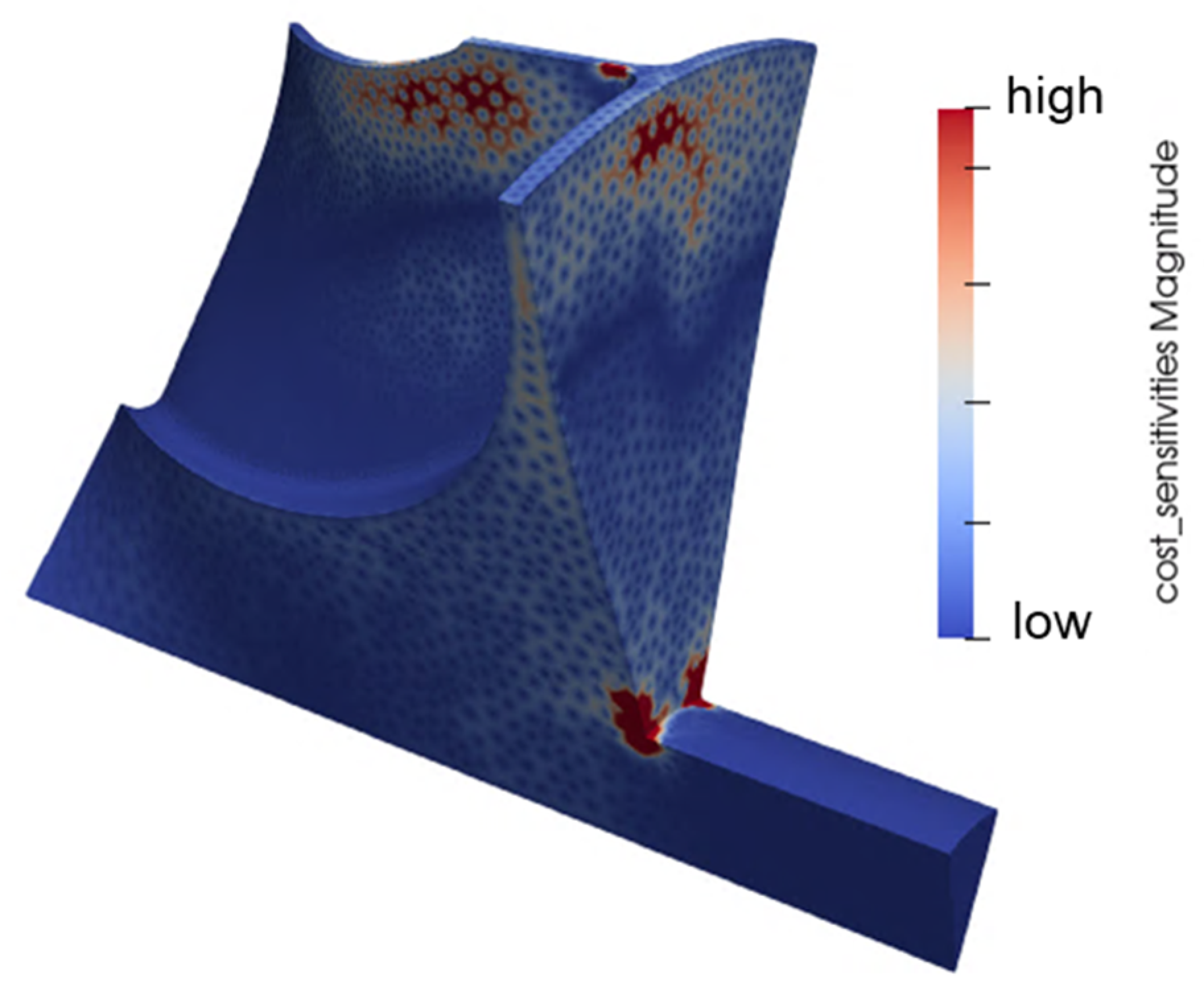
Figure 19 reveals that the maximum temperature is detected at the nodes in the region of the hub, in proximity with the leading edge. The computation of such constraint through a
p-norm function returns a marked sensitivity from the rotor back-plate thickness, whose enlargement would reduce the influence of the heat sink located at the back-plate outer surface. Similarly, an increase in blade height at the leading edge would extend the thermal path to the colder areas highlighted at the tip, while an elongation of the shaft itself would reduce the gradient field. On the contrary, an increase in the turbine shaft diameter, an advancement of the axial position of the intersection between the rotor back-plate and the shaft, and an enlargement of the blade hub thickness would favor the cooling of the hub upper region. Such sensitivities provide the descent direction for a constrained optimization problem aimed at limiting the maximum rotor temperature for the sake of extended lifetime.
Similarly, the accuracy of the adjoint structural solver sensitivities is assessed by comparison with the same gradients computed by Finite Differences. The results reported in
Figure 18b confirm the suitability of the manually differentiated framework.
Moreover, the time for the computation of the adjoint-based gradients for the heat transfer solver and the structural solver was measured. If X is the time required for the computation of the multidisciplinary workflow in primal mode and the problem accounts for n design variables, the calculation of the gradients by Finite Differences would approximately cost n ∙ X. On the contrary, the application of the adjoint method herein described costs about 8.6X for the heat transfer module and 2.3X for the structural analysis, in fair agreement with the original expectations. Such costs mostly depend on the assembly process of the differentiated system (Equation (25)) rather than the solver itself.
Finally, the loose-coupling approach adopted for the development of the CHT workflow allows the direct integration of the in-house adjoint CFD solver, and the accuracy of the computed gradients was already demonstrated by the same author.


