NREL-5MW Wind Turbine Noise Prediction by FWH-LES ^†

Abstract

This paper deals with large onshore wind turbine aeroacoustics. Noise from the NREL 5 MW device is predicted by the permeable-surface Ffowcs Williams–Hawkings equation (FWH-P), starting from the postprocessing of LES data on different acoustic surfaces $\mathcal{S}$. Their size and placement is aimed at embedding most of the aerodynamic sources of sound surrounding rotor and nacelle. Due to the presence of eddies that inevitably cross $\mathcal{S}$, this paper compares results from open and closed acoustic surfaces, and the outflow disk averaging technique. The issues related to the interpolation process of LES data on $\mathcal{S}$ is discussed as well. In order to assess the LES/FWH-P aeroacoustic platform, LES and FWH-P pressures are compared in the very-near field. It is shown that, within the limits of the discretization settings imposed by the interpolation procedure and for the Reynolds number working condition investigated herein, the lack of quadrupole sources outside the permeable surface(s) deeply affect the quality of FWH-P acoustic pressures with respect to direct LES signals.

1. Introduction

There has been substantial growth in the renewable energy field in the past few years, in particular in wind energy industry. European governments have set the mammoth target of 450 GW of offshore wind by 2050, requiring a huge effort to innovate the actual technologies and improve performance. Larger wind turbines are constantly being developed, as the generated power increases with the square of the rotor diameter. Moreover, an increase in turbine height provides more reliable access to high wind speeds and improves the capacity factor of the turbines, resulting in a lower levelised cost of energy [1]. However, this increase in size can have adverse effects on the turbine’s noise spectrum, and wind turbine acoustic noise emission may deviate from design levels due to highly variable operating conditions, causing concern among local residents and requiring reduced power production of the contributing turbines. As a matter of fact, on shore wind turbine (WT) aeroacoustics is a significant hindrance to the widespread acceptance of wind power. Radiated noise negatively impacts public opinion due to perceived annoyance, and is the reason why wind turbine acoustics are the subject of significant research.

Acoustic noise generated by modern industrial-scale wind turbines is typically dominated by aerodynamic noise, as mechanical noise is more readily reduced by careful design. For the (very low) Mach numbers relevant to wind turbines, aeroacoustic noise is in general produced by unsteady flow interacting with the rotor blades. Following [2], aerofoil self-sound mechanisms can be generally classified intotrailing edge noise due to the turbulent boundary layer, vortex shedding noise due to the laminar boundary layer, boundary layer separation noise, large-scale separation (deep stall) noise, and vortex shedding noise due to trailing edge bluntness. In addition, noise generation from blade tip vortex formation is worth mentioning. Due to this complexity, empirical or simplified formulations such as actuator line, actuator disk, or blade element momentum theory, which approximate blades as lines or disks applying forces to the fluid, are suitable for power prediction but too rough to properly predict the unsteady aerodynamic environment past the turbine and do not allow for accurate noise prediction. The literature shows that in order to reduce CPU time as much as possible, reliable wind turbine aerodynamics rely on large-eddy simulations (LES) of the wake where the turbulence model directly resolves large-scale eddies by modelling the smaller ones and thereby eliminates the extra computational cost. There is often cross-over in the above approaches, with LES solvers using actuator line or disk methods (see for instance [3,4,5,6,7]).

The aim of this paper is the assessment of a numerical framework for wind turbine aeroacoustics through the combined use of LES aerodynamics and acoustic analogy. Specifically, LES aerodynamics, where the actuator line method models the rotor blades and the immersed boundary method models the presence of the nacelle (see [8,9,10]), is used first to detect the main sources of sound, with noise levels then predicted by the acoustic analogy of Ffowcs Williams and Hawkings (FWH) [11], herein applied by the permeable-surface technique [12]. The analysis concerns the NREL 5-MW turbine in design condition. This paper is the first step in an ongoing activity with a final target of developing a consistent strategy towards noise prediction in the near/mid-field surrounding the turbine. Herein, possible strategies to mitigate fictitious signals induced by the turbine wake crossing the porous surface (end-cap problem) are proposed, among them the use of open surfaces and the disk averaging technique. Note that the truncation of the acoustic surface negates the assumption that it surrounds all the sources of noise, allowing the volume integral to be omitted with rigor. This is crucial for WT characterized by persisting wake structures far from the rotor disk, for instance, in low Reynolds number working conditions. All these aspects are discussed in the numerical results by comparing direct LES pressures and the FWH-based acoustic signals in the time and frequency domains.

2. Methodology

2.1. Large Eddy Simulation

In this work, LES is employed in order to compare the results against those obtained through the acoustic analogy. In this type of approach, the large-scale structures which depend on the geometry of the problem are resolved, whereas the small-scale fluctuations are filtered and modeled. The main advantage of using LES with respect to Direct Numerical Simulation (DNS) is its reduced computational cost. The non-dimensional filtered incompressible Navier–Stokes equations are used. The governing equations are the following:

$$\begin{array}{c}\frac{\partial u_i}{\partial t}+\frac{\partial u_i{u}_j}{\partial x_j}=-\frac{\partial p}{\partial x_i}+\frac{1}{Re}\frac{{\partial }^2{u}_i}{\partial x_j\partial x_j}-\frac{\partial {\tau }_{ij}}{\partial x_j}+F_i,\end{array}$$

(1)

$$\begin{array}{c}\frac{\partial u_i}{\partial x_i}=0,\end{array}$$

(2)

where $i,j\in$$\left\{1,2,3\right\}$ represents in a Cartesian reference frame of the components along the streamwise, wall-normal, and spanwise directions, respectively, $Re=U_{\infty }D/\nu$ is the Reynolds number, $U_{\infty }$ is the upstream inlet velocity, D is the turbine diameter, and $\nu$ is the kinematic viscosity of the fluid. These quantities are used as references for the non-dimensionalization of the equations ($x_i=X_i/D$ and $u_i=U_i/U_{\infty }$). The filtered Navier–Stokes equations differ from the non-filtered ones in the presence of the sub-grid scale (SGS) stress tensor ${\tau }_{ij}$, which describes the interaction between the large resolved and sub-grid unresolved scales. The SGS stress tensor is decomposed into the isotropic component, which is included in the “modified” filtered pressure $p^{\ast }=p+\frac{1}{3}{\tau }_{kk}$, and the anisotropic component ${\tau }_{ij}^r$. The anisotropic component is modeled following a linear eddy–viscosity approach based on Boussinesq’s hypothesis:

$${\tau }_{ij}^r={\tau }_{ij}-\frac{1}{3}{\delta }_{ij}{\tau }_{kk}=-{\nu }_r\left(\frac{\partial u_i}{\partial x_j}+\frac{\partial u_j}{\partial x_i}\right)=-2{\nu }_r{\overline{S}}_{ij},$$

(3)

where ${\overline{S}}_{ij}$ is the filtered strain rate tensor and ${\nu }_r$ is the eddy viscosity. For the SGS, we employ the Smagorinsky model; thus, the eddy viscosity assumes the following expression:

$${\nu }_r={\left(C_s\overline{\Delta }\right)}^2\sqrt{2{\overline{S}}_{ij}{\overline{S}}_{ij}},$$

(4)

where $\overline{\Delta }$ is the filtered width and $C_s=0.17$ is the Smagorinsky constant, which is chosen on the basis of [13]. Previous works ([14,15]) have reported weak dependence of the wake dynamics on the particular subgrid scale model. Therefore, we employ the Smagorinsky model here, as it has already been validated in these previous studies. The term $F_i$ in Equation (1) represents the force per unit volume exerted by the turbine blades on the fluid, as provided by the Actuator Line Method (ALM). The governing equations are resolved using a centered finite difference scheme accurate to the second order with a staggered Cartesian grid and a hybrid low-storage Runge-Kutta scheme for time integration that is accurate to the third order.

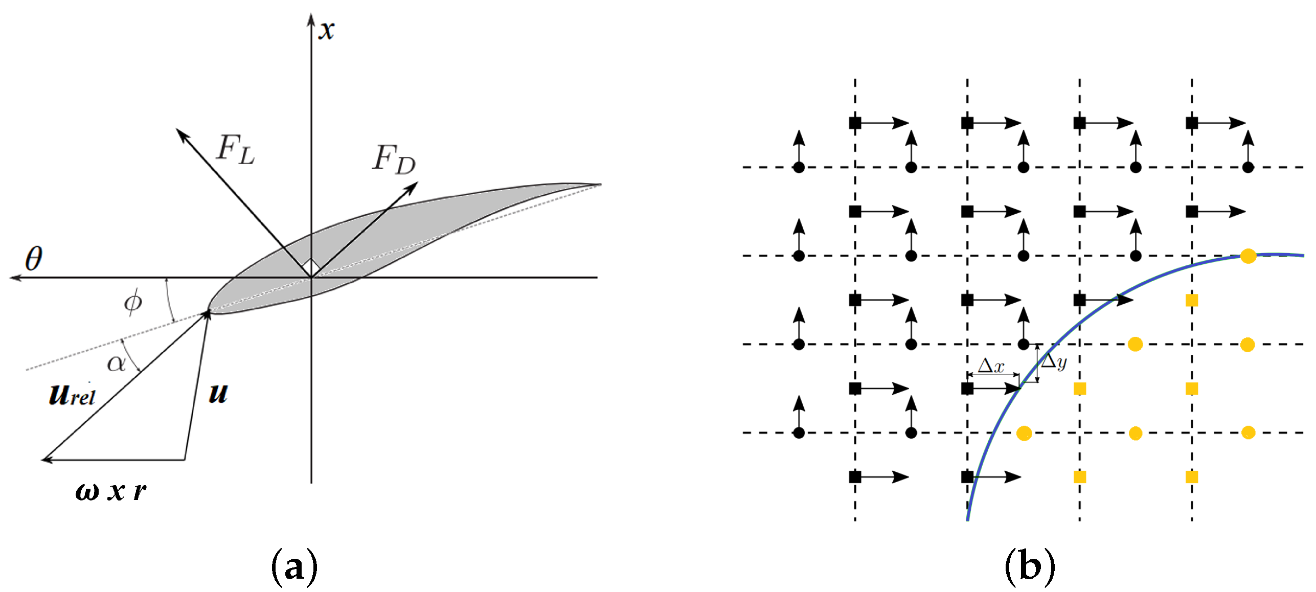
2.2. Actuator Line Model and Immersed Boundary Method

Wind turbine blades, as mentioned above, have been modeled through the Actuator Line Method (ALM) proposed by [16]. Using the ALM, blade forces are distributed along rotating lines divided into a finite number of segments along the radial direction. For each segment, the relative incoming velocity $u_{rel}$ and the angle of attack $\alpha$ are computed, as shown in Figure 1a. Then, knowing the two-dimensional characteristics of blade airfoils at each radius, as provided by the lift $C_L$ and drag $C_D$ coefficients, fluid density $\rho$, chord c, and twist angle $\mathsf{\Phi }$, it is possible to calculate the lift and drag forces per unit length as follows:

$$\begin{array}{c}{F}_L=\frac{1}{2}\rho u_{rel}^2{C}_L\left(\alpha \right)cf,\end{array}$$

(5)

$$\begin{array}{c}{F}_D=\frac{1}{2}\rho u_{rel}^2{C}_D\left(\alpha \right)cf,\end{array}$$

(6)

where the coefficient f represents the Prandtl correction factor, which takes into account the performance degradation due to tip and root vortices. The aerodynamic force F, which is the vector sum of $F_L$ and $F_D$, is projected on the fluid dynamic field by means of a Gaussian function that is spread along the surface perpendicular to the actuator line:

$$\eta =\frac{1}{{ϵ}^2\pi }exp\left[-{\left(\frac{r_{\eta }}{ϵ}\right)}^2\right]$$

(7)

where $r_{\eta }$ is the distance from the actuator line along the cross-section and $ϵ$ is a coefficient controlling the forces’ spreading. In the present work, we have assumed $\epsilon =0.025$, greater than $2\mathsf{\Delta }$, with $\mathsf{\Delta }=\sqrt{\mathsf{\Delta }{x}^2+\mathsf{\Delta }{y}^2+\mathsf{\Delta }{z}^2}$, as prescribes the classical approach [17]. Furthermore, the nacelle is described using the immersed boundary method (IBM). An approach similar to that proposed by [18] has been used. The method assigns a zero velocity $u_i=0$ to the grid points inside the solid boundary. Moreover, distances in the Navier–Stokes equations are corrected using the new metrics between the field points and the immersed points, as shown in Figure 1b.

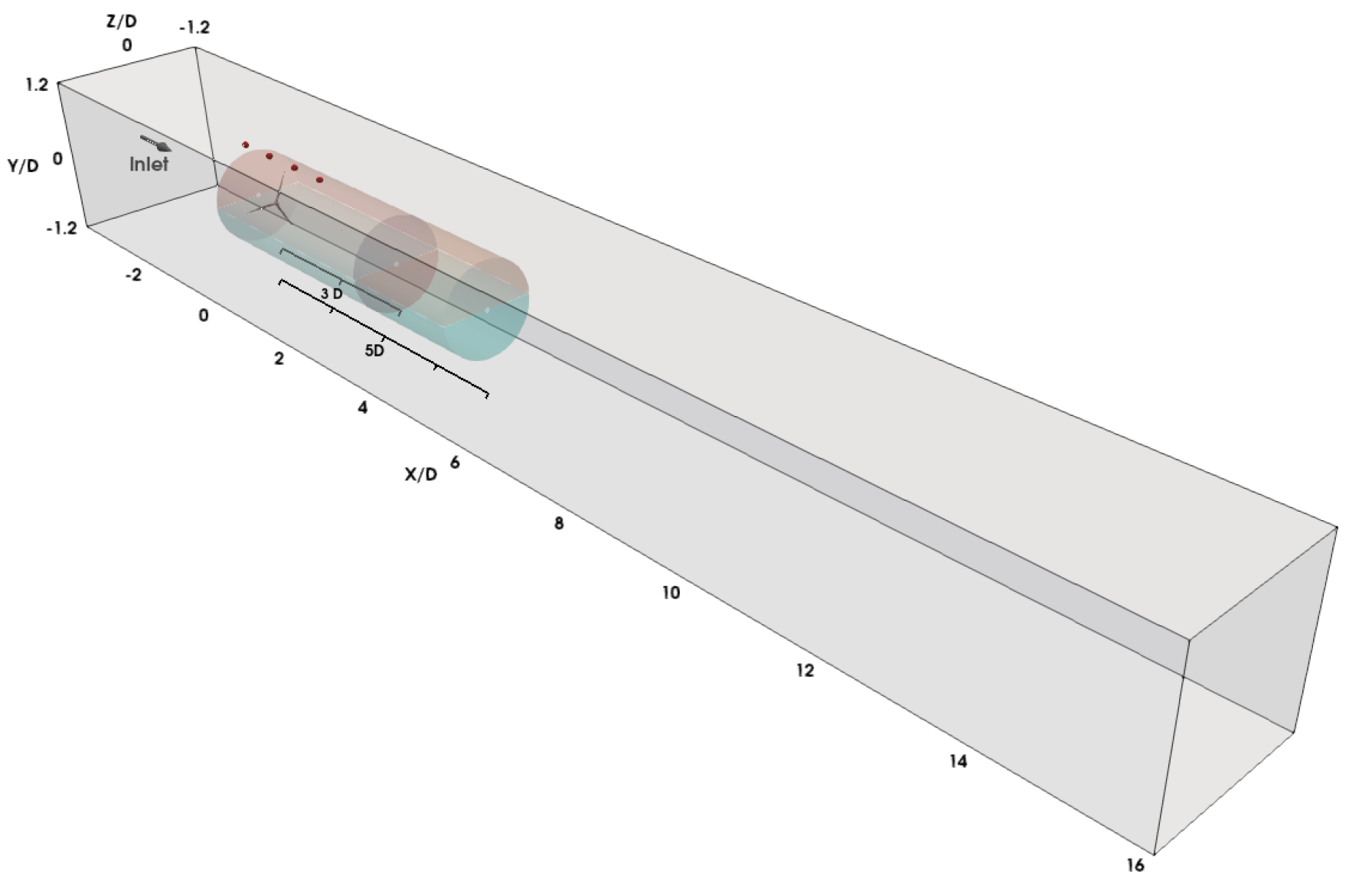
2.3. Simulation Setup

The simulation layout was arranged for describing an isolated rotor of diameter $D=126$ m along with its nacelle. The adimensional solver relates to the NREL 5 MW nominal operative conditions defined by a rated rotor speed $\omega$ of $12.1$ RPM and a rated wind speed $U_0$ equal to $11.4$ m/s, as presented in [19]. The nacelle is modeled as a capsule with an axial length of $0.083$D. The dimensions of the computational domain are (20D× 2.4D× 2.4D) in the streamwise (x), vertical (y), and spanwise (z) directions, respectively. The fluid domain has been discretized using a uniform staggered Cartesian grid chosen following a convergence analysis. The grid is made up of ($3201\times 401\times 401$), points and provides a resolution of 256 points per diameter in the streamwise direction. Inside the computational grid, two porous cylindrical grids and four acoustic observers are considered for aeroacoustic calculations (see Figure 2). The rotor is placed at $4D$ from the inlet, and is centered in the spanwise direction. A uniform laminar streamwise velocity profile defined by $U_{\infty }$ is imposed at the inlet. Moreover, a radiative boundary condition is employed at the outlet, whereas a free-slip condition is imposed on the upper and lower walls. The conditions on the side walls are periodic. The simulation runs for a Reynolds number $Re=6\times {10}^5$. The tip speed ratio is $\lambda =7$, which implies a dimensionless constant angular speed ${\displaystyle \mathrm{\Omega }=2\lambda U_0/U_{\infty }}$ of 14, with the undisturbed flow velocity $U_{\infty }$ equal to the reference velocity $U_0$.

2.4. FWH Acoustic Analogy

The Ffowcs Williams and Hawkings equation (FWHE) represents the most general form of Lighthill’s acoustic analogy ([20]). By arranging the governing equations for the flow in the form of a wave equation for the acoustic pressure, it separates sound generation mechanisms from propagation phenomena. Using the generalized functions theory, embedding the exterior flow problem in an unbounded space formulation, assuming thermodynamic transformations with negligible entropy changes, and denoting by $f(\mathbf{x},t)=0$ ($|\nabla f|=1$) the points of an arbitrary permeable surface $\mathcal{S}$ that moves with velocity $\mathbf{v}$ while enclosing a domain $\mathcal{V}$, the external acoustic pressure field $p^{\prime }=c_{{}_0}^2(\rho -{\rho }_{{}_0})$ is governed by the following form of the FWHE written in a frame of reference fixed to the undisturbed medium (see [11,12,21]):

$$\begin{array}{cc}\hfill {\overline{\square }}^2{\widehat{p}}^{\prime }& =\frac{\overline{\partial }}{\overline{\partial }t}\left[{\rho }_0\mathbf{w}·\nabla f\delta \left(f\right)\right]-\overline{\nabla }·\left[\mathbf{L}\nabla f\delta \left(f\right)\right]+\overline{\nabla }·\overline{\nabla }·\left[\mathbf{T}H\left(f\right)\right],\forall \mathbf{x}\in {\mathrm{I}\mathrm{R}}^3.\hfill \end{array}$$

(8)

Here, overlines denote generalized functions and differential operators, ${\overline{\square }}^2$ stands for the wave operator, $H\left(f\right)$ and $\delta \left(f\right)$ respectively represent the Heaviside and Dirac delta functions, ${\rho }_0$ and $c_0$ are respectively the density and sound speed of the undisturbed fluid, and ${\widehat{p}}^{\prime }=H\left(f\right)p^{\prime }$ is the generalized acoustic disturbance function, which equals the acoustic pressure field in ${\mathrm{I}\mathrm{R}}^3\setminus \mathcal{V}$ ($f>0$, $H=1$) and is zero elsewhere ($f<0$, $H=0$). The Lighthill stress tensor is $\mathbf{T}=\left[(p-p_0)\mathbf{I}-c_{{}_0}^2(\rho -{\rho }_{{}_0})\mathbf{I}+\rho (\mathbf{u}\otimes \mathbf{u})+\mathbf{V}\right]$, where $\mathbf{V}$ is the viscous stress tensor, $p_0$ is the pressure of the undisturbed medium, $\mathbf{u}$ is the fluid velocity in the air frame of reference, ${\displaystyle \mathbf{w}=(1-\frac{\rho }{{\rho }_0})\mathbf{v}+\frac{\rho }{{\rho }_0}\mathbf{u}}$, and $\mathbf{L}=\mathbf{P}+\rho (\mathbf{u}\otimes \mathbf{u})$, where $\mathbf{P}=\left[(p-p_0)\mathbf{I}+\mathbf{V}\right]$ denotes the compressive stress tensor. In order to avoid ambiguity with the formalism used in the LES modelling (where lowercase quantities denote non-dimensional variables), it should be noted here that all quantities concerning aeroacoustics are dimensional.

The application of the Green function technique turns Equation (8) into an integral form. Following [22], in the space rigidly moving with $\mathcal{V}$ with respect to the air space, and for any observer point $\mathbf{x}$ external to $\mathcal{S}$, the boundary-field integral representation for Equation (8) recasts

$$\begin{array}{c}\hfill {\displaystyle p^{\prime }(\mathbf{x},t)={\int }_{\mathcal{S}}({\mathcal{K}}_1+{\mathcal{K}}_2+{\mathcal{K}}_3)\mathrm{d}S+{\int }_{{\mathrm{I}\mathrm{R}}^3}{\mathcal{K}}_4\mathrm{d}V={\mathcal{I}}_s({\mathcal{K}}_1,{\mathcal{K}}_2,{\mathcal{K}}_3)+{\mathcal{I}}_v\left({\mathcal{K}}_4\right),}\end{array}$$

(9)

where the kernels ${\mathcal{K}}_j,j\in [1,4]$ are provided by

$$\begin{array}{ccc}\hfill {\displaystyle {\mathcal{K}}_1}& =& {\displaystyle -{\rho }_0{\left\{\mathbf{v}·\mathbf{n}\mathbf{v}·\nabla \widehat{G}+\left[\mathbf{v}·\mathbf{n}(1-\mathbf{v}·\nabla \vartheta )\right]\dot{}\widehat{G}\right\}}_{ret}}\hfill \\ \hfill {\displaystyle {\mathcal{K}}_2}& =& {\displaystyle -{\left\{\left(\mathbf{P}\mathbf{n}\right)·\nabla \widehat{G}-\left(\dot{\mathbf{P}}\mathbf{n}\right)·\nabla \vartheta \widehat{G}\right\}}_{ret}}\hfill \\ \hfill {\displaystyle {\mathcal{K}}_3}& =& {\displaystyle -\left\{\rho {\mathbf{u}}^{-}·\mathbf{n}{\mathbf{u}}^{+}·\nabla \widehat{G}+\right.{\left.\left[\rho {\mathbf{u}}^{-}·\mathbf{n}(1-{\mathbf{u}}^{+}·\nabla \vartheta )\right]\dot{}\widehat{G}\right\}}_{ret}}\hfill \\ \hfill {\displaystyle {\mathcal{K}}_4}& =& {\displaystyle {\left[\widehat{G}\nabla ·\nabla ·\left(\mathbf{T}H\right)\right]}_{ret}}\hfill \end{array}$$

in which the suffix $ret$ indicates that ${\mathcal{K}}_j$ are computed at the retarded emission time $\tau =t-\vartheta$ and $\vartheta$ denotes the time required by the acoustic disturbance released from a source point $\mathbf{y}=\mathbf{y}\left(\tau \right)$ to reach the observer at point $\mathbf{x}=\mathbf{x}\left(t\right)$, that is, the compressibility delay. In the retarded time approach followed herein, the emission time comes from the solution of the following nonlinear equation:

$$\begin{array}{c}\hfill {\displaystyle \tau =t-\frac{\left|\mathbf{x}\right(t)-\mathbf{y}(\tau \left)\right|}{c_0}}\end{array}$$

(10)

which for subsonic applications provides one root. In addition, $\mathbf{n}$ is the outward unit normal vector on $\mathcal{S}$ and $\widehat{G}$ is the retarded Green function

$$\begin{array}{c}\hfill {\displaystyle \widehat{G}={\left[-\frac{1}{4\pi r}\left(\frac{1}{1-M_r}\right)\right]}_{ret},}\end{array}$$

(11)

where $\mathbf{r}=\mathbf{x}\left(t\right)-\mathbf{y}\left(\tau \right)$, $r=\left|\mathbf{r}\right|$, ${\displaystyle M_r=\frac{\mathbf{v}}{c_0}·\widehat{\mathbf{r}}}$, the symbol $\dot{\left(\right)}$ indicates time derivation in the space rigidly connected with $\mathcal{V}$, ${\displaystyle {\mathbf{u}}^{-}=(\mathbf{u}-\mathbf{v})}$, and ${\displaystyle {\mathbf{u}}^{+}=(\mathbf{u}+\mathbf{v})}$.

Equation (9) states that the sources of sound enclosed by $\mathcal{S}$ contribute to the noise field outside it through surface integral terms, whereas the noise sources outside $\mathcal{S}$ yields an acoustic effect by the volume integral contribution of quadrupole type. Hence, if the noise sources were all encapsulated inside $\mathcal{S}$, the surface terms of Equation (9) would implicitly provide the noise induced by them, removing the need for volume integration and significantly decreasing the computational burden. Under these assumptions, CFD analysis can fruitfully solve the (very-)near field, providing the fluid properties ($\rho ,p,\mathbf{u}$) on the permeable surface. Subsequently, in this paper we neglect the quadrupole integral contribution and Equation (9) is referred to as FWH-P. Numerically, the solution of Equation (9) is obtained through a zero-order Boundary Element Method (BEM), where the permeable surface is discretized into quadrilateral panels, along which the strength of the kernels is assumed to be constant and equal to the value at the panel centroid. Validation tests and applications to propellers and wind turbines can be found in [23].

2.5. Sound Computation Procedure

In order to efficiently extrapolate near-field flow data for the far-field noise radiation in the relative frame of reference, the permeable surfaces $\mathcal{S}$ considered below are cylinders of radius R and axial length L that translate at velocity $\mathbf{v}$ = −${\mathbf{U}}_{\infty }$, where ${\mathbf{U}}_{\infty }$ is the incoming uniform free-stream velocity. The correct placement of the (closed) acoustic surface is key to guaranteeing acoustically consistent FWH-P signals. The driving criteria used for the aeroacoustic analysis rely on preliminary checking of (i) the L2 norm of the Lighthill stress tensor inside the computational domain and (ii) the location of eddies downstream of the rotor disk. Thus, the placement of $\mathcal{S}$ is a trade-off between the need to include all the quadrupole sources of sound while remaining close to the most resolved CFD zone, where the detection of the aerodynamic sources of noise is expected to be more accurate. The correct application of Equation (9) requires closed surfaces containing rotor blades, nacelles and (a part of) the wake generated downstream. To this end, the radial sizes of the cylinders guarantee that the downstream wake evolution is bounded by the lateral surface of $\mathcal{S}$ at each time step of the aerodynamic computation, although it inevitably crosses the closure end of $\mathcal{S}$, giving rise to spurious noise ([24,25,26,27,28]). Its weakening by extending $\mathcal{S}$ to the point that the vorticity/turbulence essentially decays, even by exploiting the inevitable grid coarsening, is not effective due to the rather low Reynolds number. In this paper, the outflow disk averaging technique is used to alleviate such nonphysical signals.

2.5.1. Interpolation

A set of observers co-translating rigidly with $\mathcal{S}$ in the relative frame of reference are placed in the $x-y$ plane passing through the hub and slightly above $\mathcal{S}$. These are used to conduct a comparison between LES pressure pulses and FWH-P acoustic signatures. The interface between aerodynamics and aeroacoustics is represented by the interpolation procedure that maps the time histories of ($p,\mathbf{u}$) from the CFD grid to the BEM centroids of the discretized $\mathcal{S}$ surface. Even though $\mathcal{S}$ should ideally be composed of CFD grid points to assure the best resolution and avoid possible interpolation errors (see [29]), the storage cost would be prohibitive for the investigation herein. For this reason, a devoted Paraview™-based tool is assessed to interpolate CFD data on the BEM acoustic mesh through the nearest neighbour algorithm. Note that the surface integral of Equation (9) represents the sum of a distribution of equivalent sources; thus, surface elements must be small enough to obtain a satisfactory numerical estimation of the acoustic pressure. However, BEM panel numbers cannot exceed a threshold value that makes the interpolation stage too costly.

2.5.2. Outflow Disk Averaging

This technique is based on the crude assumption that frozen turbulence is convected through the end-cap at a constant speed ${\mathbf{u}}_c$ with respect to the translating permeable surface. Let us assume a set of outflow disks regularly spaced by $\mathsf{\Delta }$ along a distance $\mathrm{\Gamma }$ downstream in the axial direction. In the frequency domain, the passage of a vortex (at time t) through the closure end of $\mathcal{S}$ is seen by an observer (OBS) rigidly translating with $\mathcal{S}$ as spurious sound, that is, as a harmonic wave at frequency $f_s$. The same vortex reaches the following outflow disk with time delay $\mathsf{\Delta }$/$|{\mathbf{u}}_c|$, and in turn the same spurious wave, as shifted by the time delay, is seen by the OBS. The parasitic non-acoustic fluctuations that translate towards the OBS at lower velocities than the sound speed may be cancelled if $1/\left(2f_s\right)=\mathsf{\Delta }/\left|{\mathbf{u}}_c\right|$. Thus, for a given choice of $\mathrm{\Gamma }$ and $\mathsf{\Delta }$ spurious signals may be cancelled in the approximate frequency range $\left[\right|{\mathbf{u}}_c|/2\mathrm{\Gamma },|{\mathbf{u}}_c|/\mathsf{\Delta }]$ by averaging the complex Fourier transforms of the signals predicted by two or more permeable surfaces. In the time domain, this is equivalent to averaging the raw time signals. Note that in the present strategy numerous planes at large separation distances help to provide largely phase-independent results that are phase-averaged to remove spurious noise. Thus, the possibility of roughly controlling spurious effects within a specified frequency range relies on the assumption of eddies frozen in a limited region outside the permeable surface. Typically, the inaccuracies due to this crude aerodynamic approximation on aeroacoustics are smaller than the discrepancies that would be obtained without any correction.

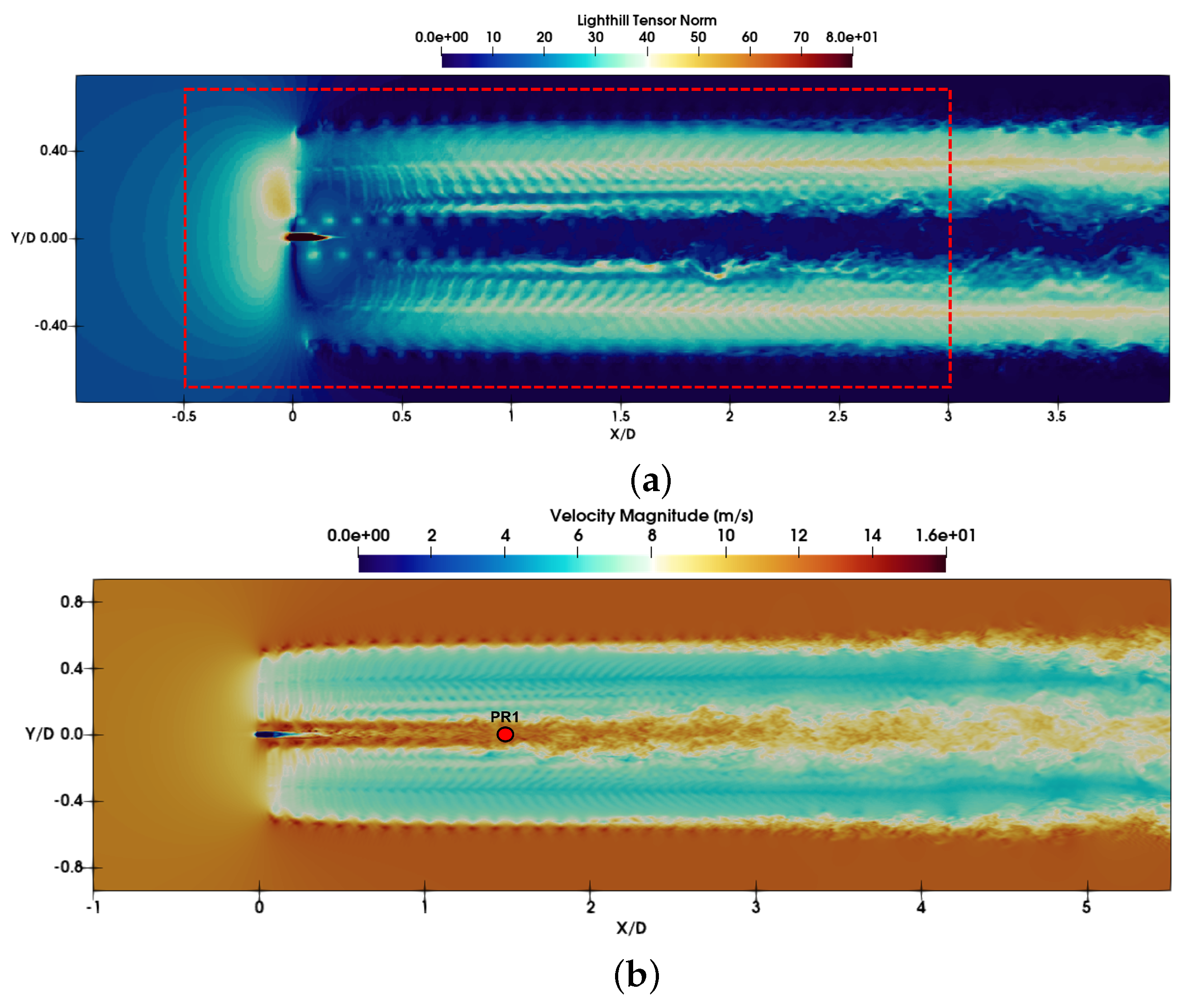
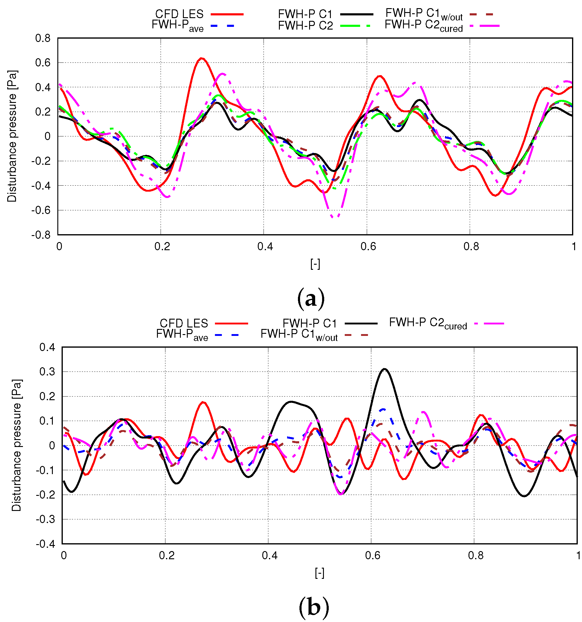
3. Numerical Results

A prior analysis of LES data has shown that the wake generated by rotor blades and nacelle is persistent. In order to assess the LES/FWH-P acoustic procedure, a porous cylinder $\mathcal{C}{}_1$ of radius $0.7D$ extending $0.5D$ upstream and $3D$ downstream of the rotor disk is first considered; see Figure 2. The snapshots of the Lighthill stress tensor norm ${\left|\right|T\left|\right|}_2$ and axial velocity magnitude inside $\mathcal{C}{}_1$ (see Figure 3a and b, respectively) clearly show the presence of wake structures crossing the outflow disk. Making reference to four microphones in the very near field which have the coordinates listed in

Table 1. Microphone coordinates.

Name	$\mathbf{x}\left[\mathbf{m}\right]$	$\mathbf{y}\left[\mathbf{m}\right]$	$\mathbf{z}\left[\mathbf{m}\right]$
Obs 1	−0.65D	0.71D	0.0
Obs 2	0.0	0.71D	0.0
Obs 3	0.65D	0.71D	0.0
Obs 4	1.3D	0.71D	0.0

, a comparison between the signals with and without the outflow disk highlights that spurious noise effects are present, in particular for the observers closer to the end-cap.

Without loss of generality, Figure 4a and b shows the results during a complete revolution of the rotor at OBS2 and OBS4, respectively, expressed in terms of the non-dimensional time $[-]=t/T$, with T being the rotor revolution period. To alleviate parasitic pressure fluctuations at the most relevant frequency $f^{\ast }$ carrying the major acoustic energy content, the disk averaging technique is applied. The PSD (Power Spectral Density) of the FWH-P pressures at all observers (not shown here for conciseness) identifies $f^{\ast }$ with the first Blade Passage Frequency (BPF), namely, 0.6 Hz. The disk averaging technique is applied by setting $\mathrm{\Gamma }=0.08D$, $\mathsf{\Delta }=0.04D$ and for an averaged flow speed $|{\mathbf{u}}_c|$ of 10 m/s estimated by the analysis of time-varying LES flowfield velocities at $x=3D$, and yields a slightly better agreement with respect to LES outcomes. However, the comparison remains unsatisfactory in that FWH-P predictions never match with them and the pressure magnitude is underestimated everywhere. Correctly, at OBS2 (placed on the rotor $xy$ plane), a dominant tonal component at the 1BPF due to the presence of the blades modulates the overall signal. Moving downstream, this contribution is less evident at OBS4, and is related to the passage of the tip vortices. In general, higher-frequency oscillations occur due to the flow past the nacelle. This is confirmed by FFT (Fast Fourier Transform) analysis of the axial velocity $1.5D$ downstream for a set of probes in the $z=0$ plane perpendicular to the x axis; for instance, at the site of probe $PR1$, which is impinged by the wake structures from the nacelle, the signal depicted in Figure 5 includes a number of significant harmonics components up to 3.23 Hz.

The unsatisfactory matching between FWH-P/LES signals may be due to the lack of aerodynamic sources of sound within the porous surface $\mathcal{S}$, that is, to the error caused by the neglected quadrupole term downstream of the closing disk. In fact, the application of the permeable surface approach for wind turbine aeroacoustics inherently leaves out from $\mathcal{S}$ an important portion of volume sources that cannot be quantified a priori. This is confirmed by the further analysis performed by a longer cylinder $5D$ long $\mathcal{C}{}_2$ downstream, with the same radius of $\mathcal{C}{}_1$. In this regard, Figure 4a highlights a slightly better agreement between LES and FWH-P signals at OBS2, though discrepancies remain evident. In light of this result, the consistency of the acoustic computation has been checked through the acoustic compatibility condition that is, ${\widehat{p}}^{\prime }=0$ for observers inside $\mathcal{S}$, where surface integral terms and the (neglected) volume contribution must be perfectly balanced. In this respect, using $\mathcal{C}{}_2$ as acoustic surface, the calculation of ${\widehat{p}}^{\prime }$ for a set of interior microphones shows that it is not zero (for brevity, this analysis is omitted here). Therefore, following [23], the neglected quadrupole contribution may be numerically estimated by embedding the selected observers inside a new cylinder $\mathcal{C}{}_3$ of radius $0.72D$ and length $5D$ with same discretization settings of $\mathcal{C}{}_2$. Looking at Figure 4a and b (the curves labeled as cured), it is evident how the lack of quadrupole sources outside the surfaces considered herein deeply affects aeroacoustic predictions when using the acoustic analogy. As a matter of fact, within the limits of the panel number used for the discretization of $\mathcal{S}$, the inclusion of the exterior volume noise contributions provides a visible enhancement to the FWH-P sound prediction. Akin to the previous results, the time shift is due to the compressibility delays (not present in the LES solver). In the frequency domain,

Table 2. OASPL at microphone locations for LES and FWH-P computations.

Name	$\mathbf{LES}$	$\mathcal{C}{}_2$ Not—Cured	$\mathcal{C}{}_2$ Cured
Obs 2	69.72 dB	65.07 dB	69.71 dB
Obs 3	63.10 dB	60.97 dB	64.13 dB
Obs 4	56.43 dB	56.44 dB	55.93 dB

shows the improvement in terms of Overall Sound Pressure Level (dB) (OASPL) at OBS2-OBS4 computed by LES and FWH-P (using $\mathcal{C}{}_2$ – not-cured – and cured) signatures.

4. Conclusions

The scope of this paper consists of the assessment of a numerical framework for wind turbine aeroacoustics through the combined use of LES aerodynamics and the permeable FWH Acoustic Analogy. For the NREL 5-MW turbine in design condition at a low Reynolds number, numerical results in the very near field demonstrate that the wake crossing the boundaries of the acoustic surface has to be carefully taken into consideration because of persistent wake structures that develop up to boundaries of the CFD domain. Possible strategies to mitigate fictitious signals induced by the end-cap problem, namely, open or closed surfaces and the disk averaging technique, seem to be ineffective. For the case investigated herein, discrepancies between direct LES pressures and FWH-P signatures are reduced only by including the noise contribution due to the external volume sources, and are otherwise neglected. Here, this is accomplished by embedding the microphones using a suitably chosen fictitious porous surface. Within the limits of the panel number used for the discretization of the permeable surface (imposed by the interpolation tool), the analysis in the time and frequency domains suggests that the permeable technique might fail and that the inclusion of volume terms could be mandatory. Further investigations are required.

References

1. Bolinger, M.; Wiser, R. Understanding wind turbine price trends in the US over the past decade. Energy Policy 2012, 42, 628–641. [Google Scholar] [CrossRef]
2. Tonin, R. Sources of wind turbine noise and sound propagation. Acoust. Aust. 2012, 40. [Google Scholar]
3. Jimenez, A.; Crespo, A.; Migoya, E.; García, J. Advances in large-eddy simulation of a wind turbine wake. J. Phys. Conf. Ser. 2007, 75, 012041. [Google Scholar] [CrossRef]
4. Porté-Agel, F.; Wu, Y.T.; Lu, H.; Conzemius, R.J. Large-eddy simulation of atmospheric boundary layer flow through wind turbines and wind farms. J. Wind Eng. Ind. Aerodyn. 2011, 99, 154–168. [Google Scholar] [CrossRef]
5. Delorme, Y.; Stanly, R.; Frankel, S.H.; Greenblatt, D. Application of actuator line model for large eddy simulation of rotor noise control. Aerosp. Sci. Technol. 2021, 108, 106405. [Google Scholar] [CrossRef]
6. Bontempo, R.; Manna, M. Effects of the approximations embodied in the momentum theory as applied to the nrel phase vi wind turbine. Int. J. Turbomach. Propuls. Power 2017, 2, 9. [Google Scholar] [CrossRef]
7. Bernardi, C.; Porcacchia, F.; Testa, C.; De Palma, P.; Leonardi, S.; Cherubini, S. Wind Turbine Aeroacustics by Large-Eddy Simulation—Acoustic Analogy Approach. In Proceeding of the 15th European Turbomachinery Conference, Budapest, Hungary, 24–28 April 2023; Paper n. ETC2023-333. Available online: https://www.euroturbo.eu/publications/conference-proceedings-repository/ (accessed on 15 November 2023).
8. De Cillis, G.; Cherubini, S.; Semeraro, O.; Leonardi, S.; De Palma, P. POD-based analysis of a wind turbine wake under the influence of tower and nacelle. Wind Energy 2021, 24, 609–633. [Google Scholar] [CrossRef]
9. Sotiropoulos, F.; Yang, X. Immersed boundary methods for simulating fluid–structure interaction Prog. Aerosp. Sci. 2014, 65, 1–21. [Google Scholar]
10. De Cillis, G.; Cherubini, S.; Semeraro, O.; Leonardi, S.; De Palma, P. The influence of incoming turbulence on the dynamic modes of an NREL-5MW wind turbine wake. Renew. Energy 2022, 183, 601–616. [Google Scholar] [CrossRef]
11. Ffowcs Williams, J.; Hawkings, D. Sound Generation by Turbulence and Surfaces in Arbitrary Motion. Phil. Trans. R. Soc. A 1969, 264, 321–342. [Google Scholar]
12. di Francescantonio, P. A new boundary integral formulation for the prediction of sound radiation. J. Sound Vib. 1997, 202, 491–509. [Google Scholar] [CrossRef]
13. De Cillis, G.; Semeraro, O.; Leonardi, S.; De Palma, P.; Cherubini, S. Dynamic-mode-decomposition of the wake of the NREL-5MW wind turbine impinged by a laminar inflow. Renew. Energy 2022, 199, 1–10. [Google Scholar] [CrossRef]
14. Ciri, U.; Salvetti, M.; Carrasquillo, K.; Santoni, C.; Iungo, G.; Leonardi, S. Effects of the subgrid-scale modeling in the large-eddy simulations of wind turbines. In Direct and Large-Eddy Simulation X; Springer: Berlin/Heidelberg, Germany, 2018; pp. 109–115. [Google Scholar]
15. Sarlak, H.; Meneveau, C.; Sørensen, J.N. Role of subgrid-scale modeling in large eddy simulation of wind turbine wake interactions. Renew. Energy 2015, 77, 386–399. [Google Scholar] [CrossRef]
16. Sørensen, J.N.; Shen, W.Z. Computation of wind turbine wakes using combined Navier-Stokes/actuator-line Methodology. In Proceedings of the 1999 European Wind Energy Conference and Exhibition, Nice, France, 1–5 March 1999; pp. 156–159. [Google Scholar]
17. Troldborg, N. Actuator Line Modeling of Wind Turbine Wakes; Technical University of Denmark: Lyngby, Denmark, 2009. [Google Scholar]
18. Orlandi, P.; Leonardi, S. DNS of turbulent channel flows with two-and three-dimensional roughness. J. Turbul. 2006, 7, N73. [Google Scholar] [CrossRef]
19. Jonkman, J.; Butterfield, S.; Musial, W.; Scott, G. Definition of a 5-MW Reference Wind Turbine for Offshore System Development; Technical report; National Renewable Energy Lab. (NREL): Golden, CO, USA, 2009.
20. Lighthill, M. On sound generated aerodynamically. I. General theory. Proc. R. Soc. A 1952, 211, 564–587. [Google Scholar]
21. Brentner, K.; Farassat, F. An Analytical Comparison of the Acoustic Analogy and Kirchhoff Formulation for Moving Surfaces. AIAA J. 1997, 36, 1379–1386. [Google Scholar] [CrossRef]
22. Testa, C.; Poggi, C.; Bernardini, G.; Gennaretti, M. Pressure-field permeable-surface integral formulations for sound scattered by moving bodies. J. Sound Vib. 2019, 459, 114860. [Google Scholar] [CrossRef]
23. Testa, C.; Porcacchia, F.; Zaghi, S.; Gennaretti, M. Study of a FWH-based permeable-surface formulation for propeller hydroacoustics. Ocean Eng. 2021, 240, 109828. [Google Scholar] [CrossRef]
24. Nitzkorski, Z.; Mahesh, K. A Dynamic end cap Technique for Sound Computation Using the Ffowcs Williams and Hawkings Equations. Phys. Fluids 2014, 26. [Google Scholar] [CrossRef]
25. Uzun, A.; Lyrintsis, A.S.; Blaisdell, G.A. Coupling of integral acoustics methods with LES for jet noise prediction. Int. J. Aeroacous. 2004, 3, 297–346. [Google Scholar] [CrossRef]
26. Rahier, G.; Prieur, J.; Vuillot, F.; Lupoglazoff, N.; Biancherin, A. Investigation of integral surface formulations for acoustic predictions of hot jets starting from unsteady aerodynamic simulations. In Proceedings of the AIAA 2003–3164, 9th AIAA/CEAS Aeroacoustics Conference, Hilton Head, SC, USA, May 12–14 2003. [Google Scholar]
27. Eastwood, S.; Tucker, P.; Xia, H. High-Performance Computing in Jet Aerodynamics, Parallel Scientific Computing and Optimization; York, S.N., Ed.; Springer Optimization and Its Applications; Springer: Berlin/Heidelberg, Germany, 2009; Volume 27, pp. 193–206. [Google Scholar]
28. Shur, M.L.; Spalart, P.R.; Strelets, M.K. Noise prediction for increasingly complex jets. Part I: Methods and tests. Int. J. Aeroacous. 2005, 4, 213–246. [Google Scholar] [CrossRef]
29. Greschner, B.; Thiele, F.; Jacob, M.C.; Casalino, D. Prediction of sound generated by a rod-airfoil configuration using EASM DES and the generalised Lighthill/FW-H analogy. Comput. Fluids 2008, 37, 402–413. [Google Scholar] [CrossRef]
Figure 1. (a) Cross-section of the blade, where θ is the tangential direction, x is the streamwise coordinate, and ω and r are the rotor angular speed and the radial position, respectively. (b) Sketch of the staggered grid near a solid shape (the blue curve); the yellow markers lie inside the solid domain, where the velocity is set to zero, while Δ x and Δ y are the distances used to calculate velocity derivatives near the solid boundary.
Ijtpp 08 00054 g001
Figure 2. CFD domain and sketch of the permeable surfaces C 1 and C 2 and the acoustic observers.
Ijtpp 08 00054 g002
Figure 3. (a) Snapshot of the Lighthill stress tensor norm | | T | | 2 ; the red dashed contour represents the trace of the porous cylinder C 1 on the longitudinal plane. (b) Snapshot of the streamwise velocity magnitude; PR1 indicates the probe, placed at the center of the wake where the axial velocity is detected.
Ijtpp 08 00054 g003
Figure 4. Comparison among LES (red solid line) and FWH-P time signals (a) at OBS2 (the disk plane) and (b) at OBS4 (downstream of the disk plane). FWH-P signatures refer to the closed porous surfaces C 1 (solid black line) and C 2 (solid green line), without the outflow disk C 1 (brown dashed line), the averaging technique (blue dashed line), and the cured signal (pink dashed line).
Ijtpp 08 00054 g004
Figure 5. Time history of the axial streamwise velocity at PR1 during a blade revolution.
Ijtpp 08 00054 g005